Face Recognition Based on Lightweight Convolutional Neural Networks

1
Institute of Microelectronics, Chinese Academy of Sciences, Beijing 100029, China
2
University of Chinese Academy of Sciences, Beijing 100049, China
*
Authors to whom correspondence should be addressed.
Information 2021, 12(5), 191; https://0-doi-org.brum.beds.ac.uk/10.3390/info12050191
Submission received: 29 March 2021
/
Revised: 22 April 2021
/
Accepted: 23 April 2021
/
Published: 28 April 2021
(This article belongs to the Section Artificial Intelligence)
Abstract
:Face recognition algorithms based on deep learning methods have become increasingly popular. Most of these are based on highly precise but complex convolutional neural networks (CNNs), which require significant computing resources and storage, and are difficult to deploy on mobile devices or embedded terminals. In this paper, we propose several methods to improve the algorithms for face recognition based on a lightweight CNN, which is further optimized in terms of the network architecture and training pattern on the basis of MobileFaceNet. Regarding the network architecture, we introduce the Squeeze-and-Excitation (SE) block and propose three improved structures via a channel attention mechanism—the depthwise SE module, the depthwise separable SE module, and the linear SE module—which are able to learn the correlation of information between channels and assign them different weights. In addition, a novel training method for the face recognition task combined with an additive angular margin loss function is proposed that performs the compression and knowledge transfer of the deep network for face recognition. Finally, we obtained high-precision and lightweight face recognition models with fewer parameters and calculations that are more suitable for applications. Through extensive experiments and analysis, we demonstrate the effectiveness of the proposed methods.
1. Introduction
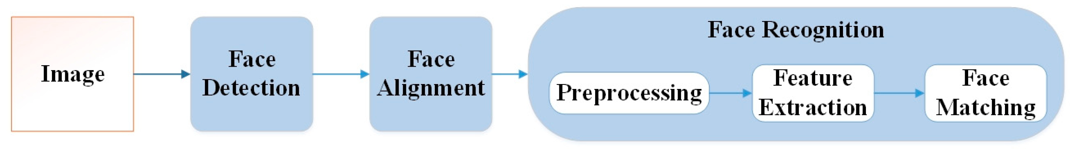
Face recognition is a technology for identifying people based on their facial features and has been widely used in different areas of daily life. Face recognition systems can be divided into several parts, including face detection, face alignment, feature extraction, and classification, as shown in Figure 1. Due to the superior performance of CNNs for extracting features, they are popular with researchers in face recognition tasks. DeepFace [1], proposed by Facebook in 2014, is one of the earliest CNN-based face recognition algorithms, and was able to achieve 97.35% accuracy on the Labeled Face in-the-Wild (LFW) dataset [2], which is close to the level of a human. Subsequently, a series of CNN-based face recognition algorithms have been successively proposed, such as DeepID [3,4,5,6], FaceNet [7], and VGGFace [8,9]. These methods overcame the constraints of traditional algorithms and improved the performance of face recognition.
Early researchers conducted various studies of network structures and datasets, including via the use of different backbones and the expansion of the datasets, and achieved face recognition through image classification. The focus of later explorations gradually shifted to the design of a suitable loss function to guide the network to learn effective features.
Prior to 2017, the loss based on the Euclidean distance, which is a metric learning method, played an important role. This approach embeds the input images into the Euclidean space and expands the inter-class distance while reducing the intra-class distance. Such methods include the contrastive loss [4], the triplet loss [7], and the center loss [10]; of these, triplet loss is used most commonly. Since 2017, the loss based on the angle or cosine margin and the normalization of features and weights have become popular, mainly modified by the softmax loss function. L-softmax [11] converts the original softmax loss into a cosine form, and multiplies the angle between features and weights by a margin. A-softmax [12] realizes the normalization of features and weights using the L2 norm. CosFace [13] improves the method of normalization and proposes a loss function with an additive cosine margin. ArcFace [14], proposed by InsightFace, introduces another additive margin, which directly adds the margin to the angle instead of to the cosine, so that the network can learn more angle characteristics.
However, the current popular face recognition algorithms are mostly based on highly precise but complex CNNs, and require significant computing resources and storage, and are difficult to deploy on mobile devices or embedded terminals. Although some highly efficient and lightweight CNNs have been directly used for face recognition tasks, the results have been unsatisfactory.
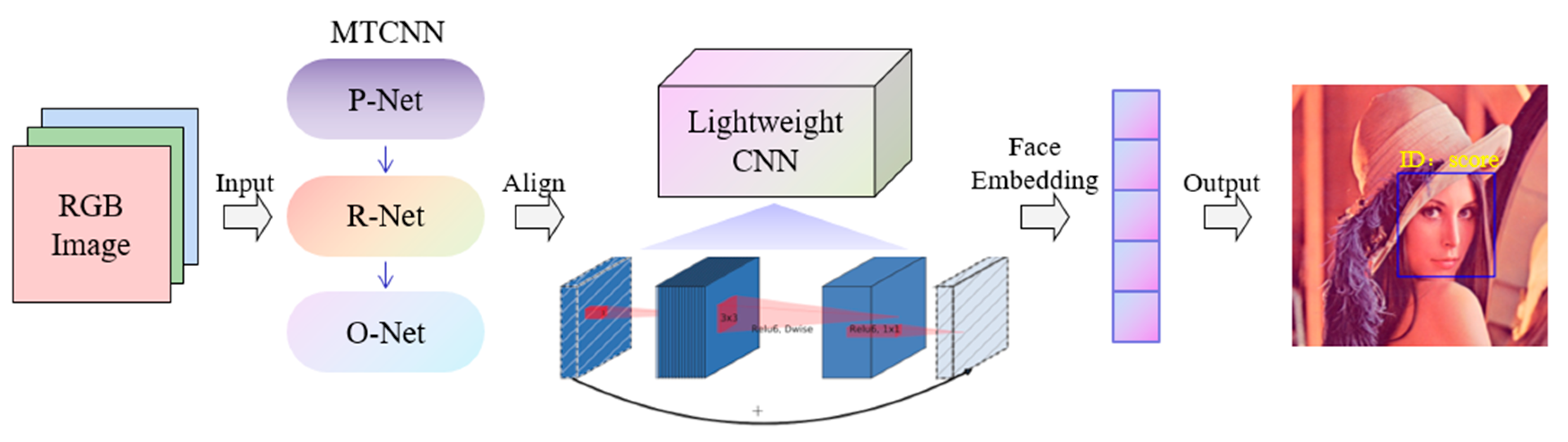
The focus of this study was the compression of the model while ensuring accuracy is maintained. We implemented face recognition using a lightweight CNN, as shown in Figure 2, making it suitable for mobile devices or embedded platforms. We improved the algorithm in terms of the network structure design, loss function, and training method. Our contributions can be summarized as follows:
- We propose three improved structures based on the channel attention mechanism: the depthwise SE module, depthwise separable SE module, and linear SE module. We applied these to the lightweight network, adding a small number of parameters and calculations, and verified their effectiveness on various datasets.
- Combined with the additive angular margin loss function, we propose a novel training method for the face recognition task, which improves the feature extraction ability of the student network, and realizes the compression and knowledge transfer of the deep network for face recognition.
- We combined the teacher–student training pattern with the improved structures using the channel attention mechanism, further improving the model’s performance on the basis of MobileFaceNet [15]. Through corresponding experiments and analysis, we promoted the accuracy on different datasets while maintaining the lightweight characteristic of the network. The results showed accuracy of 99.67% on LFW, with storage occupation of 5.36 MB and 1.35M parameters.
The remainder of this paper is organized as follows: Section 2 introduces previous related work. The proposed methods are introduced in Section 3, including network architectures and the training pattern. Section 4 describes and analyzes corresponding experiments and results. Section 5 concludes this paper.
2. Related Work
The initial development trend of CNNs was to design deeper and more complex networks to obtain higher accuracy, such as VGGNet [16], GoogleNet [17], ResNet [18], and DenseNet [19]. However, due to the continuous improvement of accuracy, the size of these models has steadily increased, thus increasing the requirements for computing equipment and storage resources, while also increasing the time required for the inference. To resolve the problem of low efficiency caused by complex models, researchers turned their attention to the design of lightweight CNNs, and proposed specific and efficient architectures to build lightweight CNNs.
SqueezeNet [20] is a relatively early and classic lightweight network, proposed at ICLR2017. It can achieve the same level of accuracy as AlexNet [21] on the ImageNet dataset with a 50-fold reduction in parameters. The fire module of SqueezeNet is the main factor that allows reduction of the number of parameters, and is comprised of a squeeze convolution module and an expand module. The squeeze module helps to compress the number of input channels, and 3 × 3 filters of the expand module are then replaced with 1 × 1 filters. ShuffleNetV1 [22] utilizes the operations of pointwise group convolution and channel shuffle to reduce parameters and calculations while maintaining accuracy. Considering the actual inference speed, ShuffleNetV2 [23] no longer uses a large number of group convolutions, but improves performance of the network through the channel split operation. MobileNetV1 [24] proposes a novel convolution operation, named depthwise separable convolutions, which splits the standard convolution into depthwise convolutions and pointwise convolutions, greatly reducing redundant calculations. MobileNetV2 [25] introduces inverted residuals and linear bottlenecks to overcome the problem of MobileNetV1. MobileNetV3 [26] combines hardware-aware network architecture search (NAS) [27] and the NetAdapt algorithm, and then improves performance through novel architecture advances. SENet [28] proposes the “Squeeze-and-Excitation” (SE) block, which adaptively recalibrates channel-wise feature responses by explicitly modelling interdependencies between channels, thus resulting in significant improvements in performance for existing state-of-the-art CNNs at a slight additional computational cost. However, when directly used for face recognition tasks, the performance of these lightweight CNNs is unsatisfactory.
To address the problems caused by complex models, researchers have designed several particular network architectures for face recognition tasks. MobileFaceNet [15] is a model based on MobileNetV2 [25] for face verification and achieves 99.55% accuracy on LFW [2]; it is also able to run on mobile phones or embedded devices in real time. MobiFace [29] replaces the global depthwise convolution of MobileFaceNet with a fully connected layer. Although the performance was improved, the number of parameters was also increased significantly. SeesawFaceNet [30] uses the Seesaw block [31] and the SE block [28] to build a more lightweight and precise model, and further optimizes MobileFaceNet. A large number of effective and lightweight CNNs remain that have not been used in the field of face recognition, such as SqueezeNet [20], ShuffleNet [22,23] and Xception [32], but have the potential for this task and deserve more attention, as introduced in [33].
In addition to the design of lightweight network architectures, common model compression methods include model pruning, model quantization, low-rank decomposition, and knowledge distillation. Several effective face recognition models are trained using methods involving knowledge distillation [34]. In [35], an enhanced version of triplet loss is proposed, named triplet distillation, which exploits the capability of a teacher model to transfer the similarity information to a small model by adaptively varying the margin between positive and negative pairs. In [36], the authors present a novel model compression approach based on the student–teacher paradigm for face recognition applications, which consists of a training teacher network at greater image resolution while student networks are trained at lower image resolutions than that of teacher network. Moreover, both the teacher network and the student network are fully convolutional networks (FCN). VarGFaceNet [37] employs an equivalence of angular distillation loss to guide the lightweight network and apply recursive knowledge distillation to relieve the discrepancy between the teacher model and the student model.
3. Proposed Approach
3.1. Network Design Strategy
In this study, the architecture of MobileFaceNet [15] was used as the benchmark to build our lightweight CNN for face recognition. The specific network architecture is shown in Table 1. The bottleneck in this approach is the inverted residual structure, which has a linear constraint introduced in MobileNetV2 [25], and expansion factors are much smaller than those in MobileNetV2 [16,25]. The inverted residual structure consists of a sequence of 1 × 1, 3 × 3, 1 × 1 convolution kernels and a shortcut that adds the input feature map to the output feature map. Because the change in the number of channels through this structure is the opposite to that of the residual structure, it is called the inverted residual structure. In addition, PReLU [38] is used as the activation function, and we perform batch normalization [39] during training. The basic components of the bottlenecks are depthwise separable convolutions, which can extract features of each channel separately. However, the key information contained in each channel is not the same. If it is simply processed in a unified manner, it is inevitable that some important information will be ignored. Thus, we introduced the channel attention mechanism to improve the architecture and propose three structures based on the “Squeeze-and-Excitation” (SE) block [28].
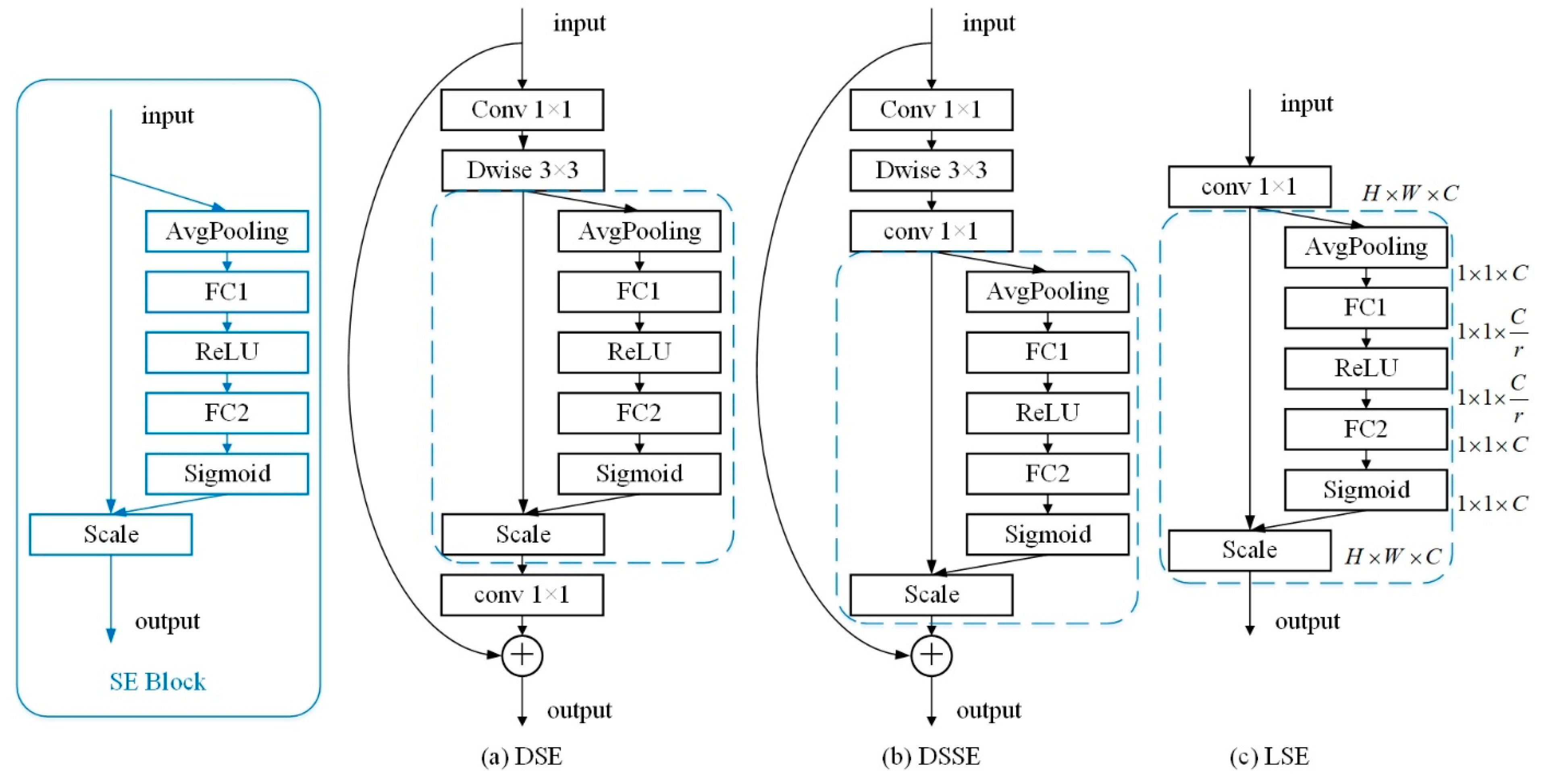
The composition of the SE block is shown in Figure 3, and its process includes three main parts. Firstly, the input feature map is passed through a squeeze operation, which utilizes a layer of global average pooling to compress the input into a 1 × 1 × C tensor such as a channel descriptor. Then, an excitation operation follows, which utilizes two fully connected layers and activation functions to learn the relevance of different channels and generate the attention weights of each channel, and the values of those weights are between (0,1). Finally, the scale operation multiplies the original input feature map with the corresponding excitation weights, and adjusts the weights of different feature maps according to the degree of dependence, thereby enhancing the attention to the key channels.
Combining the depthwise separable convolution with the SE block, we propose three structures: the depthwise SE (DSE) module, depthwise separable SE (DSSE) module, and linear SE (LSE) module, as shown in Figure 3. Because a 1 × 1 filter can maintain the existing size of the feature map and simultaneously control the number of output channels using the number of filters, it is often used to expand or reduce the number of channels. The DSE module first expands the number of channels of the input feature map through a 1 × 1 filter, then utilizes a depthwise convolution to extract features of each channel. After the features are obtained, they are input into the SE block to enhance the channel-domain attention. The DSSE module puts the SE block behind the 1 × 1 filter used to reduce the number of channels and integrate the features; that is, after completing the operation of depthwise separable convolution, the channel attention is enhanced. The DSE module focuses more on the distribution of the weights of the separate channel information, whereas the DSSE module pays attention to the overall features after the operation of depthwise separable convolution. In addition, the two structures shown in Figure 3 are used when the stride is equal to 1, and if the stride is 2, the shortcut is removed. The LSE module is composed of a 1 × 1 filter without non-linear activation and an SE block, and is utilized at the end of the entire network to realize the channel-domain attention enhancement of the finally obtained features.
We applied these structures to a lightweight convolutional neural network for face recognition. This architecture is constructed primarily by stacking a collection of improved bottlenecks. The DSE module and the DSSE module can be directly used as the bottlenecks, and the LSE is set at the end of the network. We compared and analyzed the performance of these modules. Specific experiments and results can be seen in Section 4.
3.2. Training Pattern
To further improve the performance of the lightweight model constructed in this study, we propose a novel training pattern for face recognition tasks in this section by means of knowledge distillation [34], combined with the additive angular margin loss function. Generally, large and complex neural networks have stronger capabilities in feature extraction and fitting than small and simple neural networks, and knowledge distillation can transfer knowledge between them. This often uses a large neural network as a teacher network and a small network as a student network. In the training process of the student network, the relevant features extracted by the teacher network are used to guide the training process, which can be called the teacher–student training mode. Using the teacher–student training pattern, the strong feature extraction ability and superior recognition performance of the deep CNN can be transferred to the lightweight CNN. In this manner, we can achieve model compression and improve the feature extraction ability of the student network.
Knowledge distillation can define the loss function by the difference between the logits obtained in the last layer of the network and the targets to guide the training of the model. There are two types of targets for training the student network: one is the label of the input, also called the hard target, which is a fixed value, and for which information entropy is low; the other is the output obtained by the softmax layer of the teacher network, called the soft target, which is a variable value learned by the teacher network learning and contains more information between different classes than the hard target.
We use the additive angular margin loss function introduced in ArcFace [14] as the objective function of hard targets, which is modified by softmax loss. Softmax loss is widely used in face recognition tasks, and it can be presented as:
where is the output of the fully connected layer, is the weights, is the bias, is the batch size, is the number of classes, represents the feature vector of the -th sample, and its label is . For convenience, the bias term is set to 0, and the inner product of weights and the input features is expressed in the form of cosine:
where represents the angle between weights and features. Then the ArcFace loss normalizes weights and features through L2 norm, and then multiplies a scale factor to control the magnitude of the output. To ensure the model learns distinguishing features, ArcFace introduces an additive angle margin to further restrict the training process. The final loss of hard targets is presented as follows:
where is the batch size, is the scale factor, is the number of classes, represents the label of the -th sample, represents the angle between weights and features, and is the angle margin, that is, the penalty.
In addition, the objective function of soft targets uses the additive angular margin to guide the training process. Firstly, we input the images into the teacher network to extract the feature embedding, and then input the embedding into the fully connected layer and learn the weight parameters during training. The inner product of weights and features is transformed into a cosine form, and weights and features are both regularized by L2 normalization. The scale factor and the angle margin are also introduced. We utilize the logits of the teacher network to build the loss of soft targets. After features extracted by the teacher network pass through the fully connected layer expressed in cosine form, the logits of different classes are obtained. Then, we add an angle margin to the logits related to the ground truth. In this manner, we can obtain a discriminative relationship between the output of the teacher network and the label. Furthermore, the mean square error (MSE) is used to measure the difference of logits between the teacher network and the student network. The loss function of soft targets is defined as follows:
where and represents the angles between the weights of the fully connected layer and the features extracted by the teacher network and the student network respectively, and the meaning of the other variables is the same as for the loss of hard targets. Finally, the total loss function is the weighted average of soft and hard objective functions, which is defined as follows:
where is a hyper-parameter that can adjust the proportion between soft and hard objective functions.
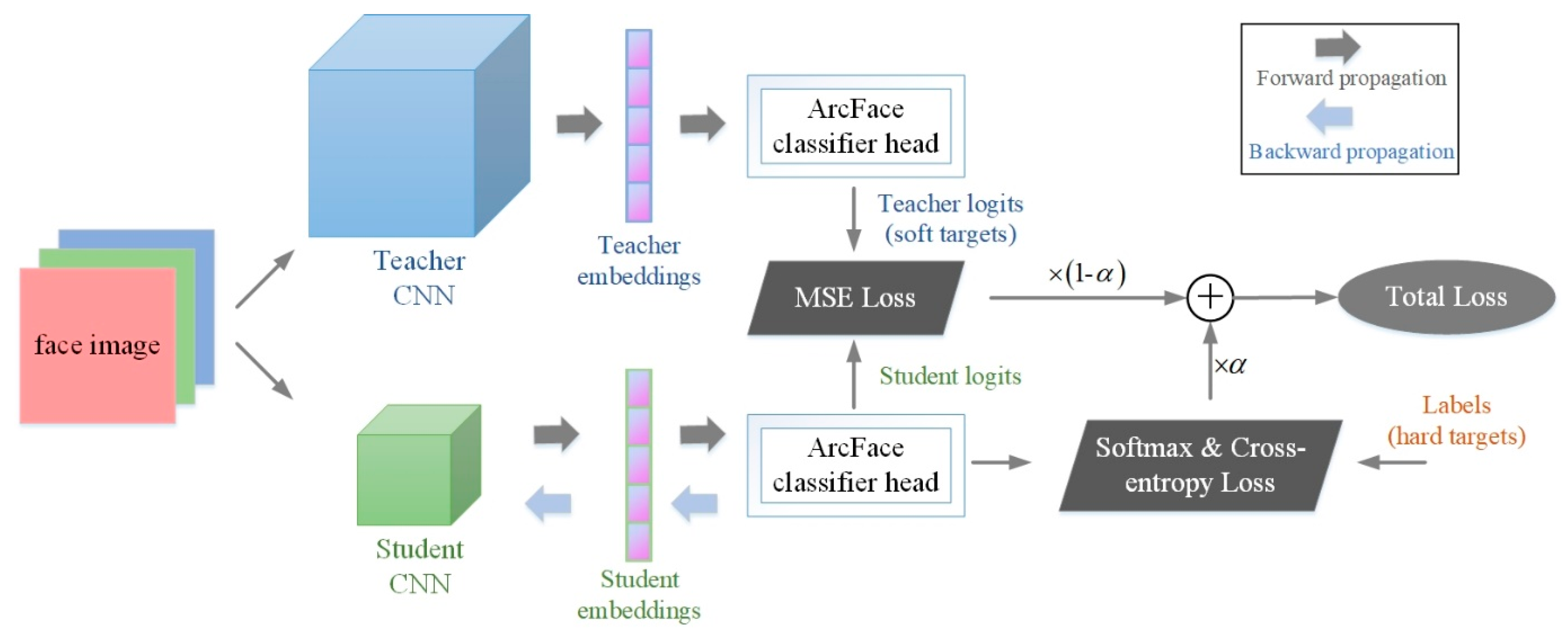
The implementation of the proposed training pattern is shown in Figure 4. We first input face images into the complex and deep teacher network, and the simple and shallow student network, and obtain the related embedding after feature extraction. Then, the embedding is input into the ArcFace classifier head with the additive angle margin, and the logits are obtained. The logits of the teacher network are used as the soft targets, and we compute the MSE between the soft targets and the logits of the student network. In addition, the labels of input images are taken as the hard targets, and we compute the softmax loss between the hard targets and the logits of the student network. The weighted average of soft and hard loss functions is the final loss, and forms the basis of the back propagation of the gradients and the parameter update of the student network. In the inference of face recognition, only the trained student model is used, which greatly reduces parameters and calculations.
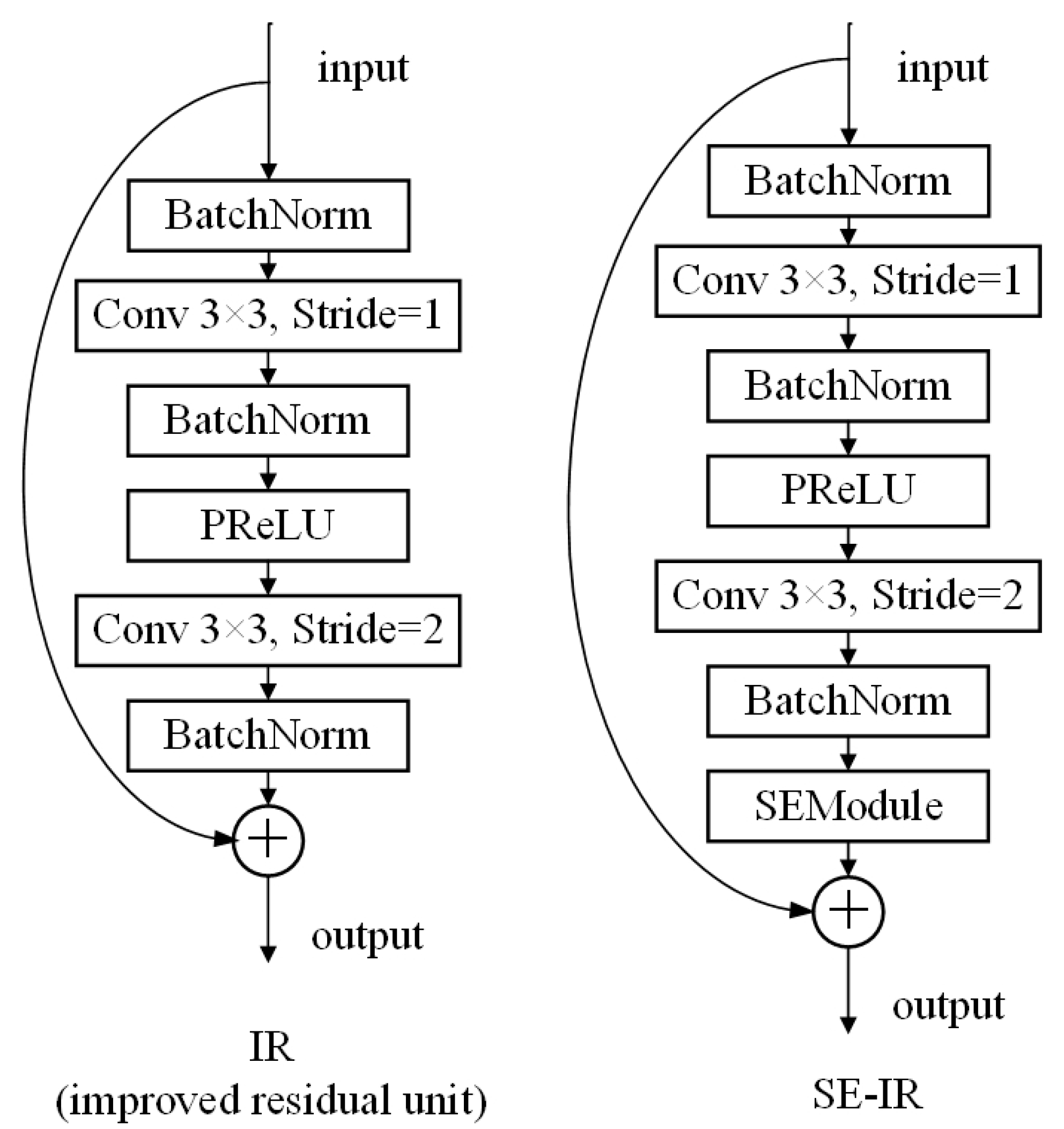
In addition, the student network used here is the lightweight CNN based on MobileFaceNet, and the teacher network is SE-ResNet50-IR [14], which is modified by ResNet [18] and stacked with improved residual (IR) units. There are 50 stacking units with the SE block in the architecture. Figure 5 shows the structure of the units.
4. Experiments and Analysis
In this section, we first introduce the datasets, evaluation metric, and the details of the training settings, then describe the performance of the baseline model, and compare and analyze the experimental results of the proposed methods.
4.1. Datasets and Evaluation Metric
We organize and list commonly used face datasets in Table 2. The face images or videos contained in these datasets were collected under unconstrained conditions, including data of different postures, ages, expressions, and lighting conditions, which are representative and universal. We employed MS1MV2 introduced in ArcFace [14] for training, which is refined from the MS-Celeb-1M [40] (MS1M) dataset. The MS1MV2 dataset contains 5.8M images from 85K identities. In addition, all face images in the dataset were detected and aligned through MTCNN [41], and the aligned faces were uniformly cropped to the size of 112 × 112. To accelerate the data reading process, we stored datasets in the form of MXNet IndexedRecord.
To effectively verify the stability of the algorithm, the test sets used in this paper involve many aspects, including the following: (1) LFW [2], composed of 13,233 images from 5749 identities with different poses and expressions, containing 6000 face pairs, is an early classic face dataset, and has become an evaluation benchmark of face recognition tasks under unconstrained conditions. In the testing process, the accuracy is obtained by comparing face pairs and determining whether they belong to the same person; (2) CALFW [44] (Cross-Age LFW), is a cross-age dataset from LFW, containing 6000 pairs of frontal faces; (3) CPLFW [43] (Cross-Pose LFW) is a cross-pose dataset from LFW and also contains 6000 face pairs; (4) CFP-FP is composed of 7000 front-profile (FP) face pairs from the CFP [45] dataset. CFP is composed of 7000 images from 500 identities, and each identity has 10 frontal images and 4 profile images. These data are divided into 10 parts, each consisting of 350 pairs from the same identity and 350 pairs from different identities; (5) CFP-FF contains 7000 front-front (FF) face pairs from CFP [45]; (6) AgeDB-30 is composed of the data with an age gap of 30 in the AgeDB [46] dataset, including 6000 face pairs; (7) VGG2-FP consists of 5000 front-profile (FP) face pairs from the VGGFace2 [9] dataset.
4.2. Implementation Details
To improve GPU utilization and accelerate the training process, we used the DataParallel function of Pytorch to implement single-host multi-GPU training, and two graphics cards were used during each training process. In addition, we used the DataLoader function of MXNet to read the IndexedRecord format datasets to speed up the entire training process. Furthermore, all images for training were faces of uniform size obtained by face detection and alignment. Before they were input into the network, they were randomly horizontally flipped and normalized into [−1,1].
During the training stage, we adopted the stochastic gradient descent (SGD) optimizer. The momentum parameter was set to 0.9, which allows accumulation of the gradient of past steps to determine the direction of gradient descent and accelerate the network learning process. According to the memory of the graphics cards, the batch size was set to 256 and the dimension of the output embedding was 512. The learning rate was initialized to 0.1, and we set three milestones. The learning rate was divided by 10 at 8, 12, and 14 epochs and the training stage was stopped at 16 epochs. The last batch of images that could not be evenly distributed was processed in a “rollover” method, which means the remaining samples are transferred to the next training epoch.
4.3. Experimental Results
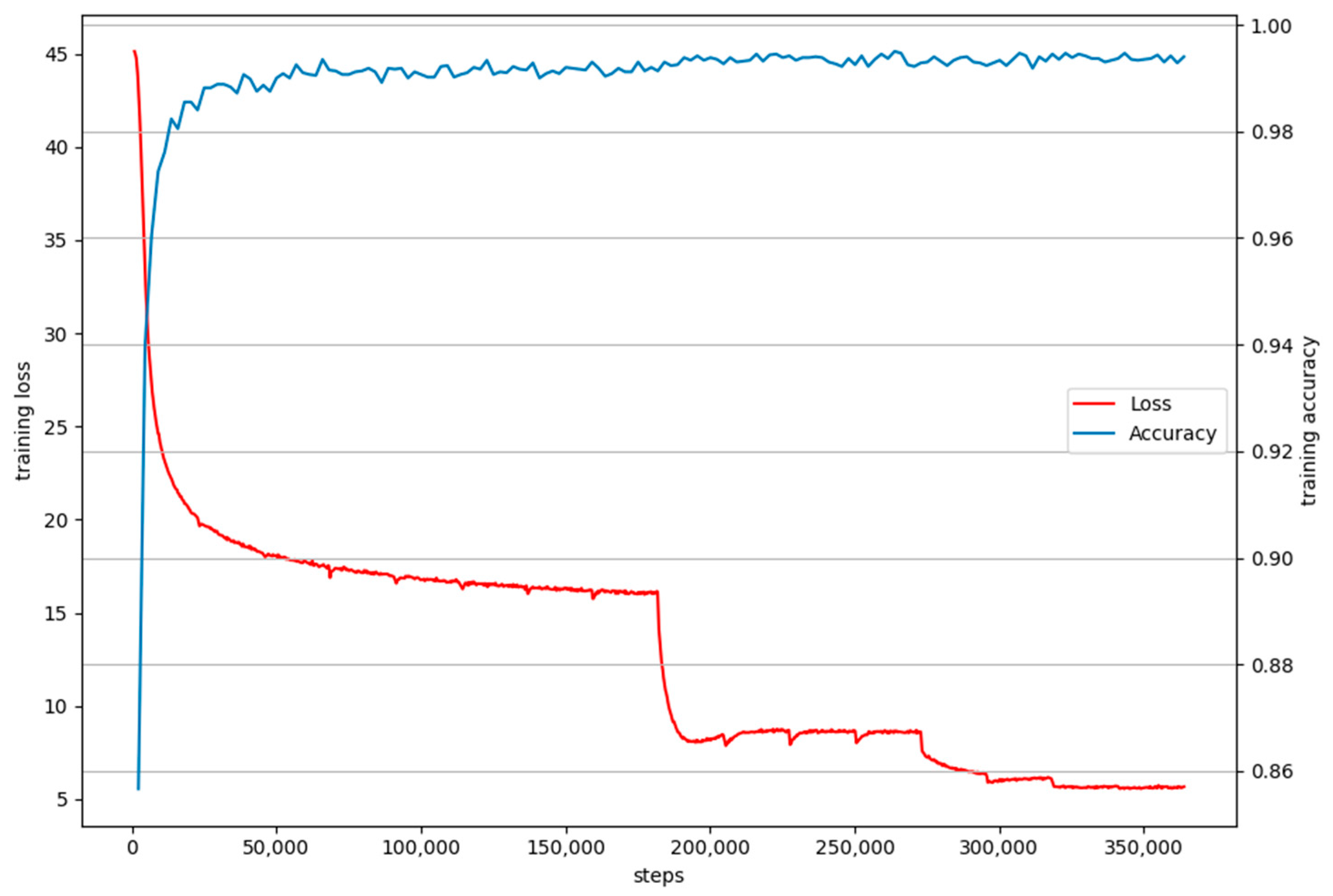
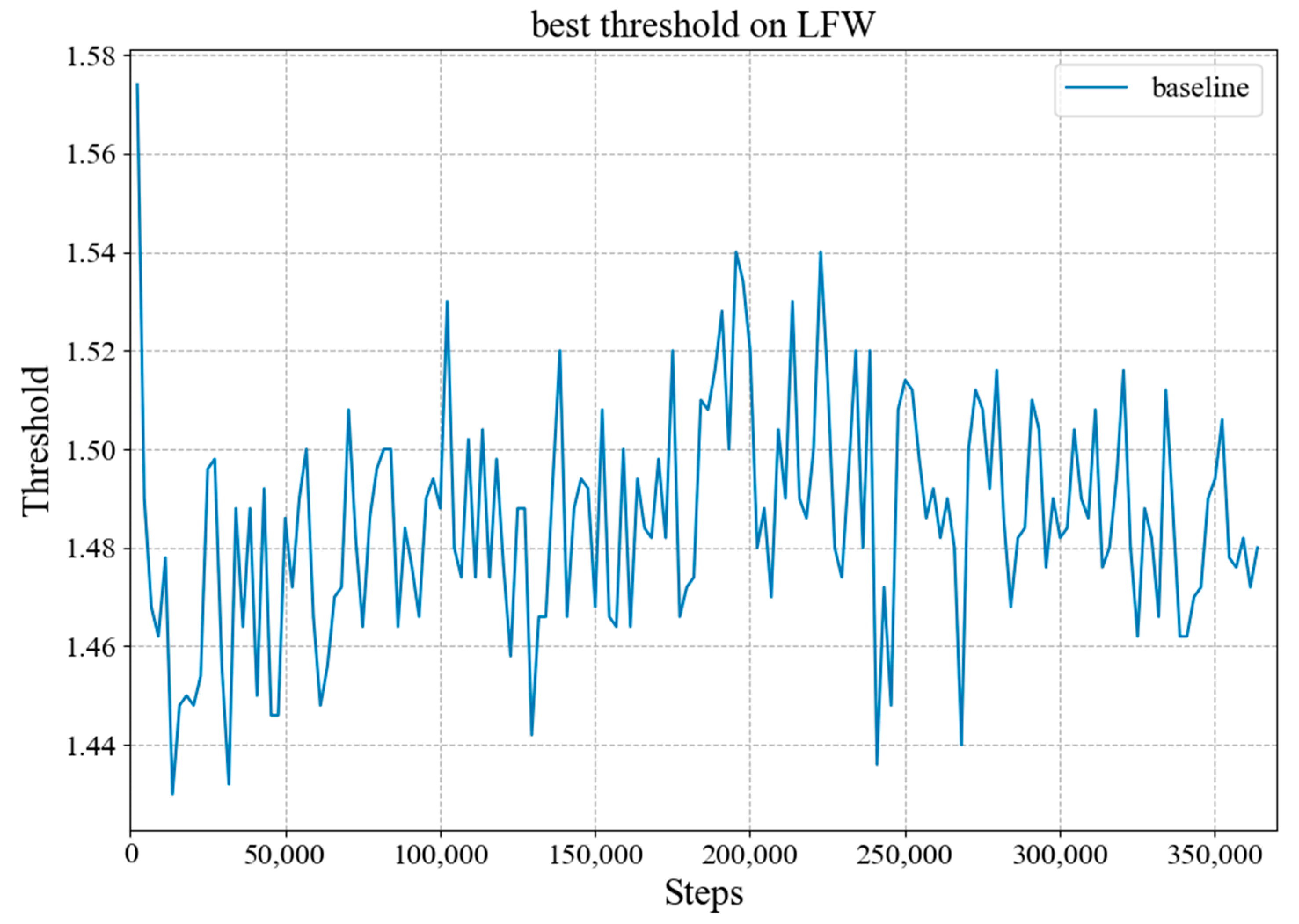
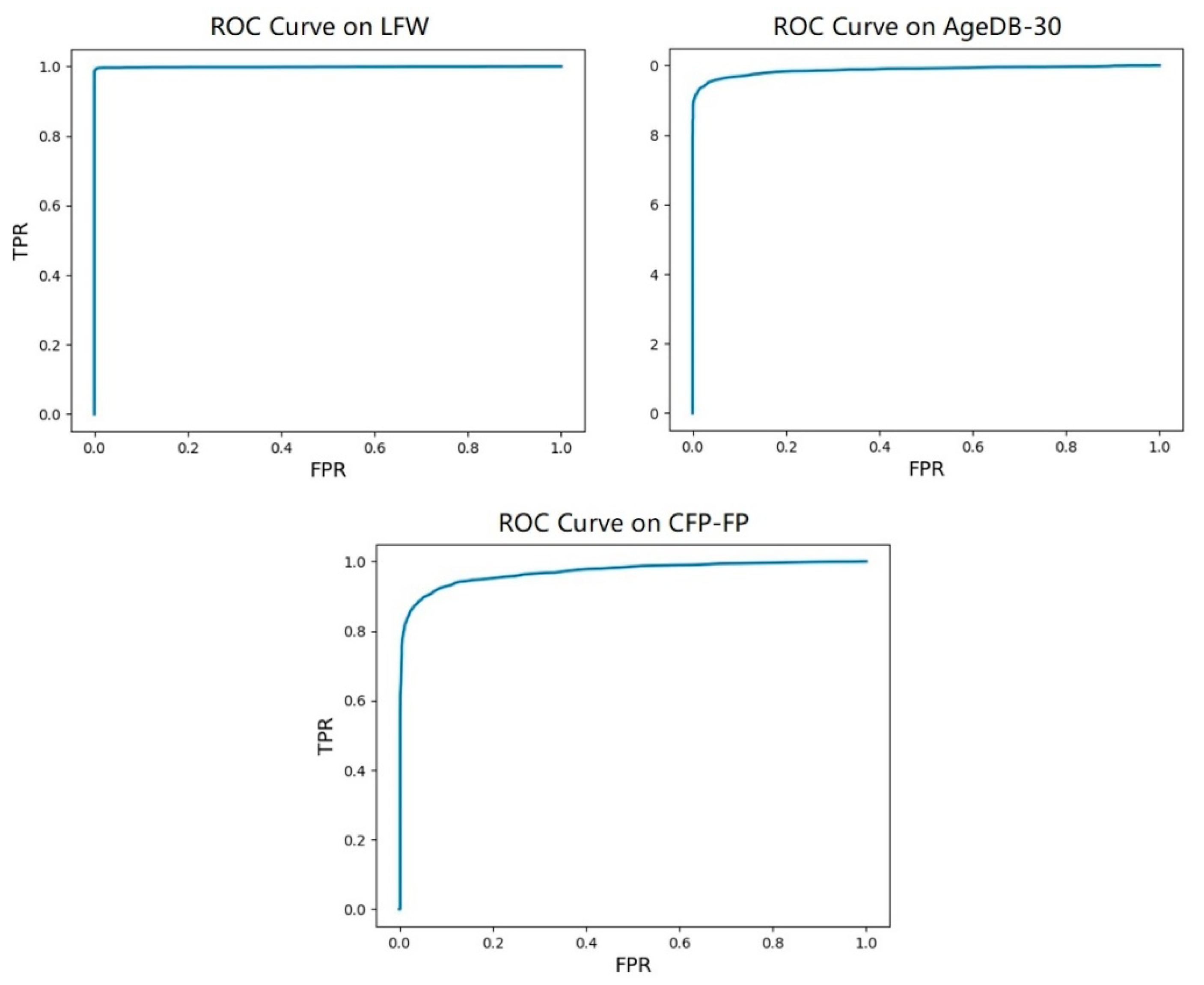
We constructed the face recognition model with the architecture shown in Table 1, and used it as the baseline. We used the ArcFace loss [14] to supervise the training process, where the scale factor was set to 64 and the angle margin was 0.5. We trained our network from scratch. To verify the training effect of the model, during training, the k-fold cross-validation result on LFW [2] was calculated. As shown in Figure 6, the curves in red and blue represent how the loss and accuracy of the baseline changed during training stage. It can be seen that the loss experiences three large drops at the milestones where the learning rate changes, and the decline in other places is relatively flat. In the process of reducing the loss through gradient backpropagation, a local minimum may occur. When the decline becomes slow, it is likely that the local minimum is encountered. We set three milestones and divided the learning rate by 10 at 8, 12, and 14 epochs. Because the batch size was set to 256 and the training set contains 5,822,653 face images, the number of steps for one training epoch was about 22,745. Therefore, when the number of steps was approximately 180,000, 280,000 and 320,000, the learning rate changed, resulting in the sudden drops of loss. In addition, the accuracy rate constantly approached 1 as the training progressed. Figure 7 shows how the best threshold of the baseline changed on LFW during training, and that the best threshold constantly changed. After calculation, the average of these thresholds was about 1.485, and the standard deviation was about 0.023. Accuracy of the baseline on each test set is shown in Table 3. The baseline occupied 4.8 MB memory and the accuracy achieved on LFW reached 99.47%. Figure 8 from left to right shows the Receiver Operating Characteristic (ROC) curve of the baseline on LFW, AgeDB-30, and CFP-FP, the performance is consistent with the accuracy rate and was best on LFW.
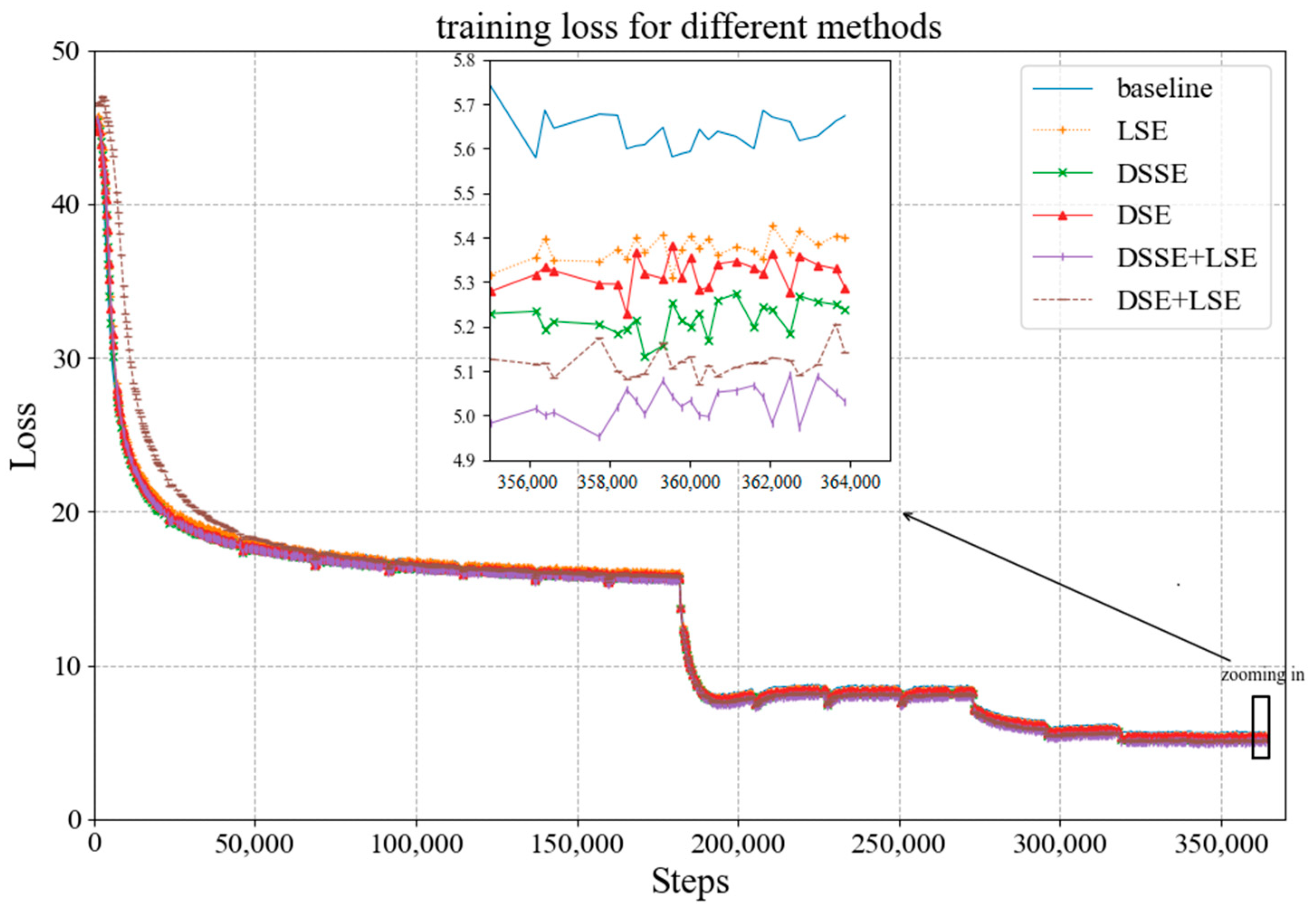
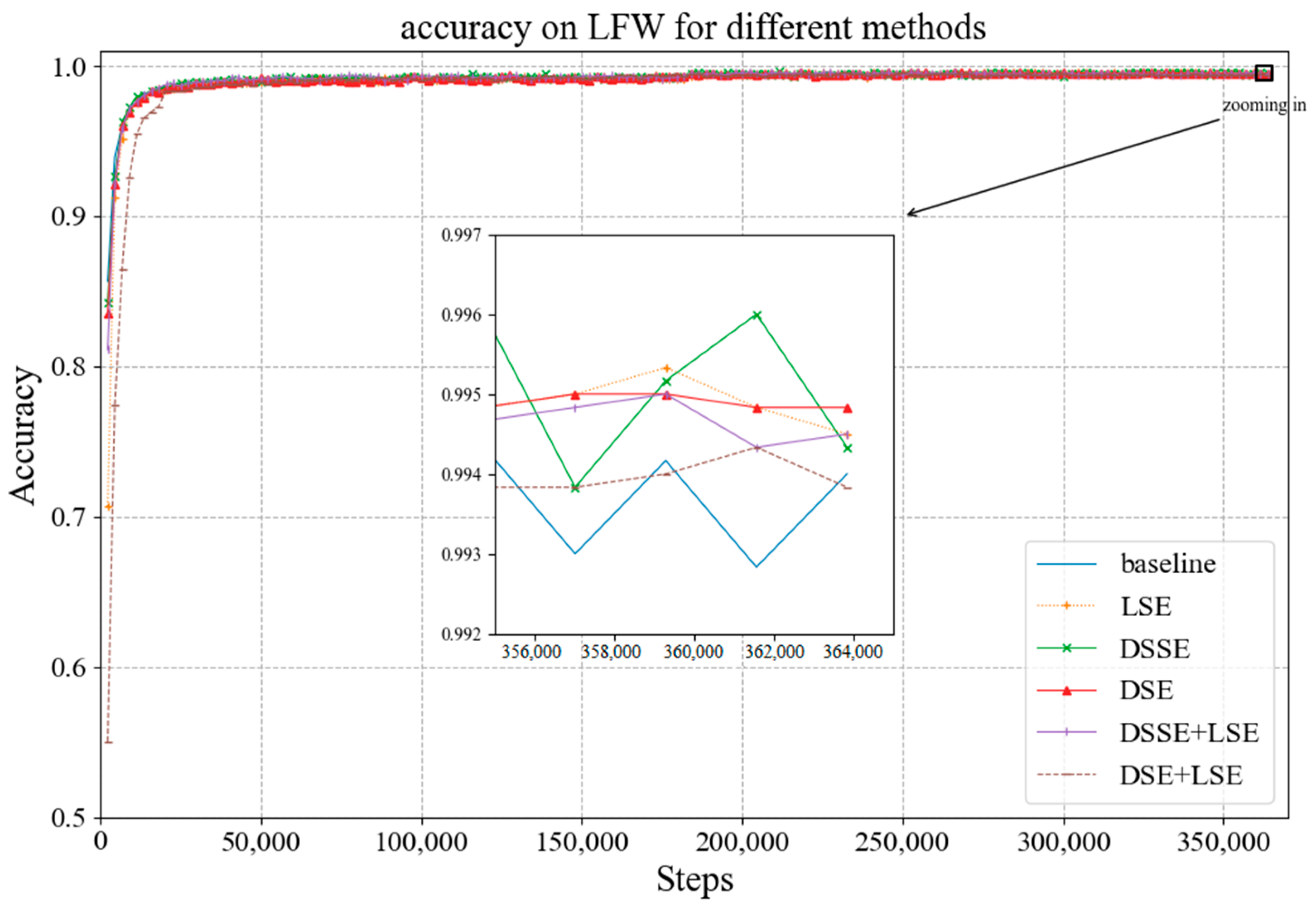
Combining the improved structures based on the channel attention mechanism proposed in Section 3.1, i.e., the depthwise SE (DSE) module, depthwise separable SE (DSSE) module, and linear SE (LSE) module, we conducted corresponding experiments of training and testing. Figure 9 and Figure 10 show the change in loss and accuracy during training after utilizing different modules in the architecture. In the figures, the blue curve represents the baseline, the orange represents the model with LSE, the green represents the model with DSSE, the red represents the model with DSE, the purple represents the model with DSSE and LSE, and the brown represents the model with DSE and LSE. It can be seen from Figure 9 that the overall trend of training loss with different modules is consistent with the baseline. When magnifying the curves at the end, we can see that after utilizing the SE blocks, the training loss is lower than that of the baseline. Moreover, the model with LSE has the lowest drop in training loss, whereas the training loss with DSSE and LSE has the maximum drop. Figure 10 shows that accuracy of each model on LFW is higher than that of the baseline, and all are above 99%.
The test results of the models with different SE modules on each test set are shown in Table 4. According to the average accuracy, the overall recognition effect of the model with DSSE and LSE is the best, and that of the model with LSE is the worst, and worse than that of the baseline, whereas other models have the best recognition effect on some test sets. Because LSE is a linear SE module, the channel attention mechanism is only used in the last linear layer of the model, and its effect is minimal on the entire network. Therefore, it is difficult to improve the model using LSE alone. When we combine the model with LSE and DSSE, it achieves the best average accuracy because the channel attention enhancement is set after 1 × 1 convolutions. Compared with the model that only uses DSSE, its feature extraction ability is further improved. The feature map is extracted and integrated through depthwise separable convolutions or linear 1 × 1 convolutions, and the features contain deeper semantic information, which is more conducive to the extraction of facial features. In addition, the STD column represents the standard deviation value of each model on different test sets. It can be seen that compared to the baseline, the STD values of our proposed models are smaller. As introduced in Section 4.1, different test sets contain face pairs with different attributes, and the standard deviation can reflect the generalization ability and robustness of the model on these test sets. The smaller the value, the better the performance.
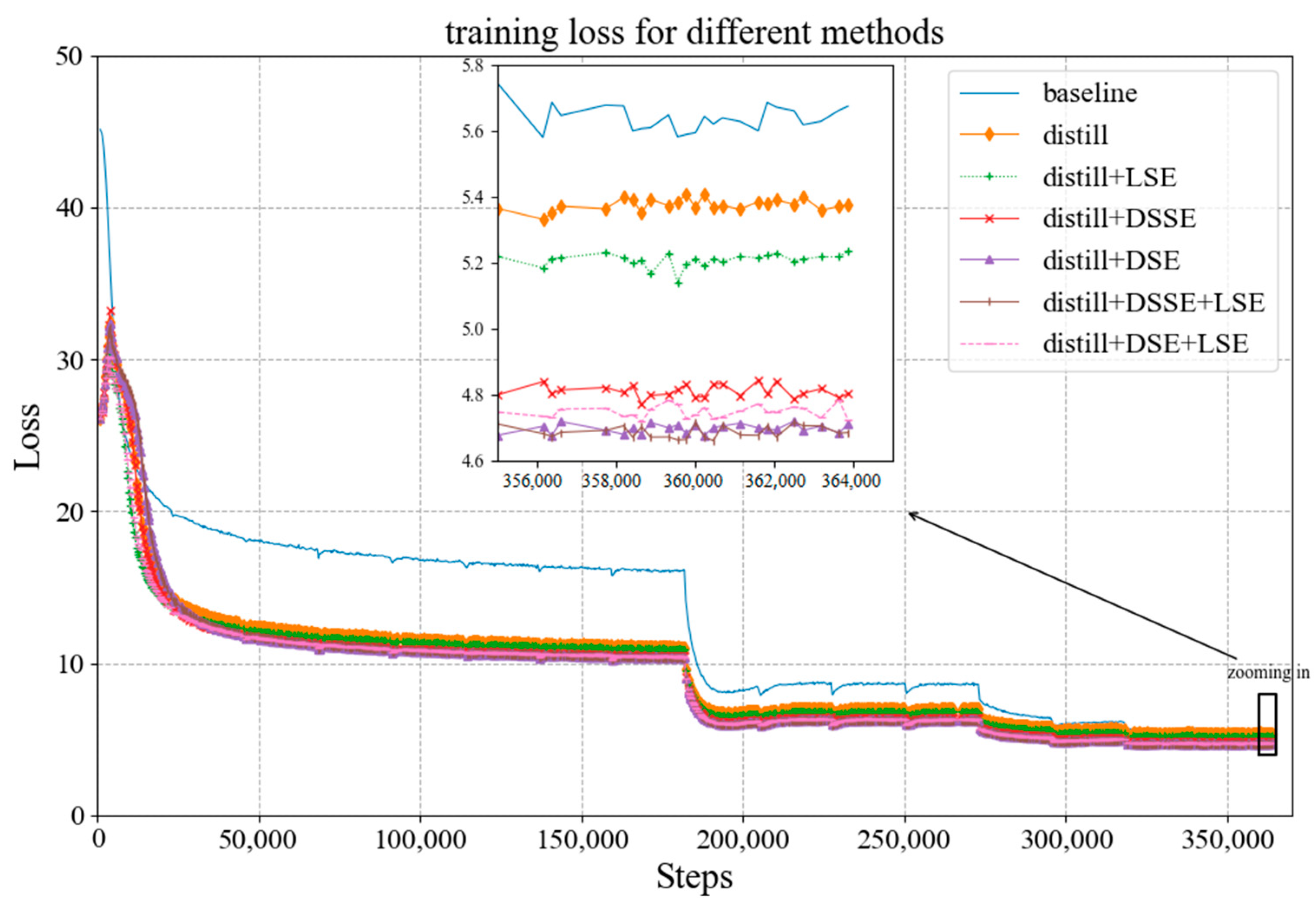
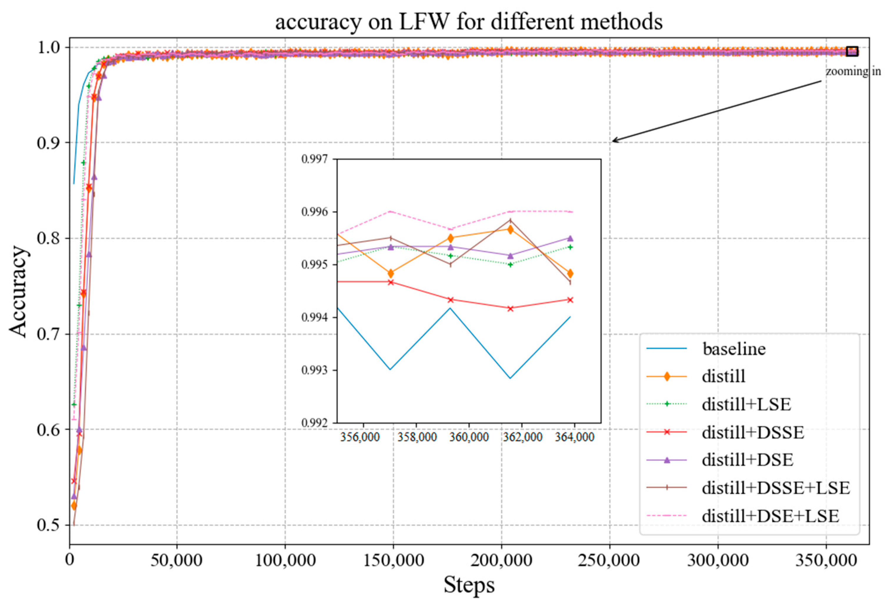
On the basis of the above experiments, we conducted experiments with the teacher–student training pattern proposed in Section 3.2. In the proposed pattern, when the weight parameter is set to 0.5, the losses of the soft and hard targets are at the same level, and the training effect is best. Figure 11 and Figure 12 show, respectively, the curves of the loss and accuracy of the model with different SE modules during the training stage in the teacher–student training pattern. In the figures, the blue curve represents the baseline, the orange curve represents the baseline in the proposed training pattern, and other curves represent the models with different modules in the proposed training pattern. As Figure 11 shows, the decline of training loss in the teacher–student training pattern is significantly greater than that of the baseline, which indicates that the teacher–student training pattern proposed in this paper introduces supervision information from the teacher network and speeds up the convergence of the student network. In addition, when zooming in on the curves at the end, it can be seen that the loss of models in the teacher–student training pattern is lower than that of the baseline. The loss decline of the baseline in the teacher–student training pattern is the smallest, and the decline of the model with LSE in the proposed training pattern is second, where the model with DSE in the teacher–student training pattern has the maximum loss drop. It can be seen in Figure 12 that the accuracy of each model on LFW is higher than that of the baseline, and they are all above 99%. Moreover, the model with DSE and LSE in the teacher–student training pattern can achieve the highest accuracy on LFW.
The test results of the models with different SE modules in the teacher–student training pattern on each test set are shown in Table 5. According to the average accuracy, the overall recognition effect of the model with DSE is the best in the training pattern, and that of the model with LSE is the worst, whereas other models have the best recognition effect on some test sets. It can be seen that the accuracy of the model trained in the teacher–student training pattern is improved compared to that of the baseline, so the training pattern proposed in this paper effectively compresses the knowledge of the teacher network to the student network, and improves the feature extraction ability of the student network. In addition, we used SE-ResNet50-IR [14] as the teacher network, which is introduced in Section 3.2, and the SE blocks are located at the end of each stacking units and act after 3 × 3 convolutions. The model with DSE in the teacher–student training pattern places the SE blocks after depthwise convolutions composed of 3 × 3 filters. Compared with other models, the architecture of the model with DSE is more consistent with that of the teacher model, so it integrates the feature extraction ability of the teacher network to the greatest extent, and not only inherits the features of the similar structure, but also learns features extracted by other structures. In addition, the STD column represents the standard deviation value of each model on different test sets. It can be seen that compared to the baseline, the STD values of our proposed models are smaller. As introduced in Section 4.1, different test sets contain face pairs with different attributes, and the standard deviation can reflect the generalization ability and robustness of the model on these test sets. The smaller the value, the better the performance.
Table 6 compares the performance indicators of different models involved in this paper, including the model size, inference time, and the number of parameters and calculations. The MACs represent the multiply–accumulate operations that contain a multiplication and an addition, which can be used to measure the computational complexity of the model. The inference time is measured on the same GPU platform through the Event function of CUDA. To overcome the randomness of a single sample, we first count the inference time of 600 samples and then compute the mean and variance. It can be seen in the table that we improved the performance of the model and increased the number of parameters by 0.15 MB at most, and the inference time only increased by about three milliseconds, whereas the computational complexity remained almost unchanged. Therefore, we achieved the research goal of making the model as lightweight as possible while maintaining the recognition accuracy. Because the models based on the teacher–student training pattern are only different from those obtained in the normal training pattern in terms of the training method, and the architectures are not changed, the model size and the number of parameters and calculations are the same as those in the normal training pattern, and the results are not repeated here. Table 7 compares the performance of the model proposed in this paper with the state-of-the-art (SOTA) face recognition models, including complex models and lightweight models. It can be seen that the model proposed is competitive in model size and recognition accuracy.
5. Conclusions
In this study, we improved face recognition algorithms based on lightweight CNNs in terms of the aspects of network architecture and the training pattern. We proposed three improved structures based on the channel attention mechanism: the depthwise SE module, depthwise separable SE module, and linear SE module. Compared with the baseline, the models with improved structure achieved higher accuracy on the test sets, adding only a small number of parameters and calculations. Combined with the additive angular margin loss function, we proposed a novel training method for the face recognition task. The feature extraction ability of the student network was improved with the supervision of the teacher network. Not only was the convergence of the student network accelerated, but the recognition accuracy was also improved, while maintaining the lightweight characteristic of the network. Furthermore, we combined the teacher–student training pattern with the improved structures, and further improved the performance of the recognition model, making it more suitable for mobile devices or embedded terminals. Experimental results showed that the proposed methods are effective.
In future research, methods of pruning and quantization can be used to further compress the model. In addition, the algorithm can utilize NAS [27] to ensure the model autonomously searches for more appropriate structures and learns more representative features. Furthermore, because of the particularity of the features of the human face, a special attention mechanism for face recognition tasks can be designed to improve performance.
Author Contributions
Conceptualization, W.L. and J.C.; methodology, W.L. and J.C.; software, W.L. and L.Z.; validation, W.L.; formal analysis, W.L.; investigation, W.L.; resources, W.L., L.Z. and J.C.; data curation, W.L.; writing—original draft preparation, W.L.; writing—review and editing, W.L., L.Z. and J.C.; visualization, W.L.; supervision, L.Z. and J.C.; project administration, L.Z. and J.C.; funding acquisition, L.Z. and J.C. All authors have read and agreed to the published version of the manuscript.
Funding
This research was supported by NSFC(U1832217).
Institutional Review Board Statement
Not applicable.
Informed Consent Statement
Informed consent was obtained from all subjects involved in the study.
Data Availability Statement
The data presented in this study are available on request from the corresponding author.
Conflicts of Interest
The authors declare no conflict of interest.
References
- Taigman, Y.; Yang, M.; Ranzato, M.A.; Wolf, L. Deepface: Closing the gap to human-level performance in face verification. In Proceedings of the IEEE Conference on Computer Vision and Pattern Recognition, Columbus, OH, USA, 24–27 June 2014; pp. 1701–1708. [Google Scholar]
- Huang, G.B.; Mattar, M.; Berg, T.; Learned-Miller, E. Labeled faces in the wild: A database forstudying face recognition in unconstrained environments. In Proceedings of the Workshop on Faces in ‘Real-Life’ Images: Detection, Alignment, and Recognition, Marseille, France, 12–18 October 2008. [Google Scholar]
- Sun, Y.; Wang, X.; Tang, X. Deep learning face representation from predicting 10,000 classes. In Proceedings of the IEEE Conference on Computer Vision and Pattern Recognition, Columbus, OH, USA, 24–27 June 2014; pp. 1891–1898. [Google Scholar]
- Sun, Y.; Wang, X.; Tang, X. Deep learning face representation by joint identification-verification. arXiv 2014, arXiv:1406.4773. [Google Scholar]
- Sun, Y.; Wang, X.; Tang, X. Deeply learned face representations are sparse, selective, and robust. In Proceedings of the IEEE Conference on Computer Vision and Pattern Recognition, Boston, MA, USA, 7–12 June 2015; pp. 2892–2900. [Google Scholar]
- Sun, Y.; Liang, D.; Wang, X.; Tang, X. Deepid3: Face recognition with very deep neural networks. arXiv 2015, arXiv:1502.00873. [Google Scholar]
- Schroff, F.; Kalenichenko, D.; Philbin, J. Facenet: A unified embedding for face recognition and clustering. In Proceedings of the IEEE Conference on Computer Vision and Pattern Recognition, Boston, MA, USA, 7–12 June 2015; pp. 815–823. [Google Scholar]
- Parkhi, O.M.; Vedaldi, A.; Zisserman, A. Deep Face Recognition. In Proceedings of the British Machine Vision Conference, Swansea, UK, 7–10 September 2015. [Google Scholar]
- Cao, Q.; Shen, L.; Xie, W.; Parkhi, O.M.; Zisserman, A. Vggface2: A dataset for recognising faces across pose and age. In Proceedings of the 2018 13th IEEE International Conference on Automatic Face & Gesture Recognition (FG 2018), Xi’an, China, 15–19 May 2018; pp. 67–74. [Google Scholar]
- Wen, Y.; Zhang, K.; Li, Z.; Qiao, Y. A discriminative feature learning approach for deep face recognition. In European Conference on Computer Vision; Springer: Cham, Switzerland, 2016; pp. 499–515. [Google Scholar]
- Liu, W.; Wen, Y.; Yu, Z.; Yang, M. Large-margin softmax loss for convolutional neural networks. arXiv 2016, arXiv:1612.02295. [Google Scholar]
- Liu, W.; Wen, Y.; Yu, Z.; Li, M.; Raj, B.; Song, L. Sphereface: Deep hypersphere embedding for face recognition. In Proceedings of the IEEE Conference on Computer Vision and Pattern Recognition, Honolulu, HI, USA, 21–26 June 2017; pp. 212–220. [Google Scholar]
- Wang, F.; Cheng, J.; Liu, W.; Liu, H. Additive margin softmax for face verification. IEEE Signal Process. Lett. 2018, 25, 926–930. [Google Scholar] [CrossRef] [Green Version]
- Deng, J.; Guo, J.; Xue, N.; Zafeiriou, S. Arcface: Additive angular margin loss for deep face recognition. In Proceedings of the IEEE/CVF Conference on Computer Vision and Pattern Recognition, Long Beach, CA, USA, 15–20 June 2019; pp. 4690–4699. [Google Scholar]
- Chen, S.; Liu, Y.; Gao, X.; Han, Z. Mobilefacenets: Efficient cnns for accurate real-time face verification on mobile devices. In Chinese Conference on Biometric Recognition; Springer: Cham, Switzerland, 2018; pp. 428–438. [Google Scholar]
- Simonyan, K.; Zisserman, A. Very deep convolutional networks for large-scale image recognition. arXiv 2014, arXiv:1409.1556. [Google Scholar]
- Szegedy, C.; Liu, W.; Jia, Y.; Sermanet, P.; Reed, S.; Anguelov, D.; Erhan, D.; Vanhoucke, V.; Rabinovich, A. Going deeper with convolutions. In Proceedings of the IEEE Conference on Computer Vision and Pattern Recognition, Boston, MA, USA, 7–12 June 2015; pp. 1–9. [Google Scholar]
- He, K.; Zhang, X.; Ren, S.; Sun, J. Deep residual learning for image recognition. In Proceedings of the IEEE Conference on Com-puter Vision and Pattern Recognition, Las Vegas, NV, USA, 27–30 June 2016; pp. 770–778. [Google Scholar]
- Huang, G.; Liu, Z.; Van Der Maaten, L.; Weinberger, K. Densely connected convolutional networks. In Proceedings of the IEEE Conference on Computer Vision and Pattern Recognition, Honolulu, HI, USA, 21–26 June 2017; pp. 4700–4708. [Google Scholar]
- Iandola, F.N.; Han, S.; Moskewicz, M.W.; Ashraf, K.; Dally, W.J.; Keutzer, K. SqueezeNet: AlexNet-level accuracy with 50x fewer parameters and <0.5 MB model size. arXiv 2016, arXiv:1602.07360. [Google Scholar]
- Krizhevsky, A.; Sutskever, I.; Hinton, G.E. Imagenet classification with deep convolutional neural networks. Adv. Neural Inf. Process. Syst. 2012, 25, 1097–1105. [Google Scholar] [CrossRef]
- Zhang, X.; Zhou, X.; Lin, M.; Sun, J. Shufflenet: An extremely efficient convolutional neural network for mobile devices. In Proceedings of the IEEE Conference on Computer Vision and Pattern Recognition, Salt Lake City, UT, USA, 18–23 June 2018; pp. 6848–6856. [Google Scholar]
- Ma, N.; Zhang, X.; Zheng, H.T.; Sun, J. Shufflenet v2: Practical guidelines for efficient cnn architecture design. In Proceedings of the European Conference on Computer Vision (ECCV), Munich, Germany, 8–14 September 2018; pp. 116–131. [Google Scholar]
- Howard, A.G.; Zhu, M.; Chen, B.; Kalenichenko, D.; Wang, W.; Weyand, T.; Andreetto, M.; Adam, H. Mobilenets: Efficient convolutional neural networks for mobile vision applications. arXiv 2017, arXiv:1704.04861. [Google Scholar]
- Sandler, M.; Howard, A.; Zhu, M.; Zhmoginov, A.; Chen, L. Mobilenetv2: Inverted residuals and linear bottlenecks. In Proceedings of the IEEE Conference on Computer Vision and Pattern Recognition, Salt Lake City, UT, USA, 18–23 June 2018; pp. 4510–4520. [Google Scholar]
- Howard, A.; Sandler, M.; Chu, G.; Chen, L.; Chen, B.; Tan, M.; Wang, W.; Zhu, Y.; Pang, R.; Vasudevan, V.; et al. Searching for mobilenetv3. In Proceedings of the IEEE/CVF International Conference on Computer Vision, Seoul, Korea, 27–28 October 2019; pp. 1314–1324. [Google Scholar]
- Tan, M.; Chen, B.; Pang, R.; Vasudevan, V.; Sandler, M.; Howard, A.; Le, Q.V. Mnasnet: Platform-aware neural architecture search for mobil. In Proceedings of the IEEE/CVF Conference on Computer Vision and Pattern Recognition, Seoul, Korea, 27–28 October 2019; pp. 2820–2828. [Google Scholar]
- Hu, J.; Shen, L.; Sun, G. Squeeze-and-excitation networks. In Proceedings of the IEEE Conference on Computer Vision and Pattern Recognition, Salt Lake City, UT, USA, 18–23 June 2018; pp. 7132–7141. [Google Scholar]
- Duong, C.N.; Quach, K.G.; Jalata, I.; Le, N.; Luu, K. Mobiface: A lightweight deep learning face recognition on mobile devices. In Proceedings of the 2019 IEEE 10th International Conference on Biometrics Theory, Applications and Systems (BTAS), Tampa, FL, USA, 23–26 September 2019; pp. 1–6. [Google Scholar]
- Zhang, J. SeesawFaceNets: Sparse and robust face verification model for mobile platform. arXiv 2019, arXiv:1908.09124. [Google Scholar]
- Zhang, J. Seesaw-Net: Convolution Neural Network with Uneven Group Convolution. arXiv 2019, arXiv:1905.03672. [Google Scholar]
- Chollet, F. Xception: Deep learning with depthwise separable convolutions. In Proceedings of the IEEE Conference on Computer Vision and Pattern Recognition, Honolulu, HI, USA, 21–26 June 2017; pp. 1251–1258. [Google Scholar]
- Wang, M.; Deng, W. Deep face recognition: A survey. arXiv 2018, arXiv:1804.06655. [Google Scholar]
- Hinton, G.; Vinyals, O.; Dean, J. Distilling the knowledge in a neural network. arXiv 2015, arXiv:1503.02531. [Google Scholar]
- Feng, Y.; Wang, H.; Hu, H.R.; Yu, L.; Wang, W.; Wang, S. Triplet distillation for deep face recognition. In Proceedings of the 2020 IEEE International Conference on Image Processing (ICIP), Abu Dhabi, United Arab, 25–28 October 2020; pp. 808–812. [Google Scholar]
- Karlekar, J.; Feng, J.; Wong, Z.S.; Pranata, S. Deep face recognition model compression via knowledge transfer and distillation. arXiv 2019, arXiv:1906.00619. [Google Scholar]
- Yan, M.; Zhao, M.; Xu, Z.; Zhang, Q.; Wang, G.; Su, Z. Vargfacenet: An efficient variable group convolutional neural network for lightweight face recognition. In Proceedings of the IEEE/CVF International Conference on Computer Vision Workshops, Seoul, Korea, 27–28 October 2019. [Google Scholar]
- He, K.; Zhang, X.; Ren, S.; Sun, J. Delving deep into rectifiers: Surpassing human-level performance on imagenet classification. In Proceedings of the IEEE International Conference on Computer Vision, Santiago, Chile, 11–18 December 2015; pp. 1026–1034. [Google Scholar]
- Ioffe, S.; Szegedy, C. Batch normalization: Accelerating deep network training by reducing internal covariate shift. In Proceedings of the International Conference on Machine Learning, Lille, France, 6–11 July 2015; pp. 448–456. [Google Scholar]
- Guo, Y.; Zhang, L.; Hu, Y.; He, X.; Gao, J. Ms-celeb-1m: A dataset and benchmark for large-scale face recognition. In European Conference on Computer Vision; Springer: Cham, Switzerland, 2016; pp. 87–102. [Google Scholar]
- Zhang, K.; Zhang, Z.; Li, Z.; Qiao, Y. Joint face detection and alignment using multitask cascaded convolutional networks. IEEE Signal Process. Lett. 2016, 23, 1499–1503. [Google Scholar] [CrossRef] [Green Version]
- Yi, D.; Lei, Z.; Liao, S.; Li, S. Learning face representation from scratch. arXiv 2014, arXiv:1411.7923. [Google Scholar]
- Zheng, T.; Deng, W. Cross-pose lfw: A database for studying cross-pose face recognition in unconstrained environments. Beijing Univ. Posts Telecommun. Tech. Rep. 2018, 5. Available online: http://www.whdeng.cn/CPLFW/Cross-Pose-LFW.pdf (accessed on 25 April 2021).
- Zheng, T.; Deng, W.; Hu, J. Cross-age lfw: A database for studying cross-age face recognition in unconstrained environments. arXiv 2017, arXiv:1708.08197. [Google Scholar]
- Sengupta, S.; Chen, J.C.; Castillo, C.; Patel, V.M.; Chellappa, R.; Jacobs, D.W. Frontal to profile face verification in the wild. In Proceedings of the 2016 IEEE Winter Conference on Applications of Computer Vision (WACV), Lake Placid, NY, USA, 7–9 March 2016; pp. 1–9. [Google Scholar]
- Moschoglou, S.; Papaioannou, A.; Sagonas, C.; Deng, J.; Kotsia, I.; Zafeiriou, S. Agedb: The first manually collected, in-the-wild age database. In Proceedings of the IEEE Conference on Computer Vision and Pattern Recognition Workshops, Honolulu, HI, USA, 21–26 June 2017; pp. 51–59. [Google Scholar]
- Wolf, L.; Hassner, T.; Maoz, I. Face recognition in unconstrained videos with matched background similarity. In Proceedings of the CVPR 2011, Colorado Springs, CO, USA, 20–25 June 2011; pp. 529–534. [Google Scholar]
- Kemelmacher-Shlizerman, I.; Seitz, S.M.; Miller, D.; Brossard, E. The megaface benchmark: 1 million faces for recognition at scale. In Proceedings of the IEEE Conference on Computer Vision and Pattern Recognition, Las Vegas, NV, USA, 27–30 June 2016; pp. 4873–4882. [Google Scholar]
- Wu, X.; He, R.; Sun, Z.; Tan, T. A light cnn for deep face representation with noisy labels. IEEE Trans. Inf. Forensics Secur. 2018, 13, 2884–2896. [Google Scholar] [CrossRef] [Green Version]
Figure 1.
Face recognition system.

Figure 2.
Face recognition based on a lightweight CNN.

Figure 3.
SE block (in the blue box) and three improved structures based on the channel attention mechanism. (a) depthwise SE (DSE) module, (b) depthwise separable SE (DSSE) module, (c) linear SE (LSE) module. Conv with capital letter represents a convolution module with a nonlinear activation function PReLU and the BN layer. Conv without capital letter represents the convolution module that does not use a nonlinear activation function. Dwise represents the depthwise convolution.

Figure 4.
Workflow of the proposed teacher–student training method. Firstly, face images are input to the deep teacher network and the lightweight student network, separately, and the related embedding after feature extraction is obtained. Then, the embedding is input into the ArcFace classifier head with the additive angle margin, and the logits are obtained. We compute the MSE between the soft targets and the logits of the student network, and compute the softmax loss between the hard targets and the student logits. The weighted average of soft and hard loss functions is the final loss, and forms the basis of the back propagation of the gradients and the parameter update of the student network.

Figure 5.
The structure of the IR unit and SE-IR block. The left IR unit means the improved residual unit, and the right SE-IR represents the improved residual unit combined with the SE block.
Figure 5.
The structure of the IR unit and SE-IR block. The left IR unit means the improved residual unit, and the right SE-IR represents the improved residual unit combined with the SE block.

Figure 6.
The curves of training loss and accuracy on LFW of the baseline.

Figure 7.
The best threshold of the baseline on LFW during the training stage.

Figure 8.
The ROC curves of the baseline on LFW, AgeDB-30, and CFP-FP.

Figure 9.
Training loss curves of the models with different SE modules.

Figure 10.
Accuracy curves of the models with different SE modules.

Figure 11.
Training loss curves of the models with different modules in the proposed training pattern.
Figure 11.
Training loss curves of the models with different modules in the proposed training pattern.

Figure 12.
Accuracy curves of the models with different modules in the proposed training pattern.


Table 1.
MobileFaceNet [15] architecture. Each line describes an operator composed of convolutional kernels and the operators in the table are executed from top to bottom in the process of network inference. The “Input” column corresponds to the size of the input feature map, which is calculated by the operators of the previous layer; the columns of t, c, n, and s correspond to the parameters of each operator. The parameter t is the expansion factor, the parameter c is the number of output channels, the parameter n represents the number of repetitions, and the parameter s represents stride, which means the sliding step of the convolution kernel, and can be used to down-sample the input feature map.
| Input | Operator | t | c | n | s |
|---|---|---|---|---|---|
| 112 × 112 × 3 | conv3 × 3 | - | 64 | 1 | 2 |
| 56 × 56 × 64 | depthwise conv3 × 3 | - | 64 | 1 | 1 |
| 56 × 56 × 64 | bottleneck | 2 | 64 | 5 | 2 |
| 28 × 28 × 64 | bottleneck | 4 | 128 | 1 | 2 |
| 14 × 14 × 128 | bottleneck | 2 | 128 | 6 | 1 |
| 14 × 14 × 128 | bottleneck | 4 | 128 | 1 | 2 |
| 7 × 7 × 128 | bottleneck | 2 | 128 | 2 | 1 |
| 7 × 7 × 128 | conv1 × 1 | - | 512 | 1 | 1 |
| 7 ×7 × 512 | linear GDConv7 × 7 | - | 512 | 1 | 1 |
| 1 × 1 × 512 | linear conv1 × 1 | - | 128 | 1 | 1 |
Table 2.
Commonly used face datasets.
| Datasets | ids | Images/Videos | Type |
|---|---|---|---|
| CASIA-WebFace [42] | 10K | 0.5M | train |
| MS-Celeb-1M [40] | 100K | 10M | train |
| VGGFace [8] | 2.6K | 2.6M | train |
| VGGFace2 [9] | 9.1K | 3.3M | train and test |
| LFW [2] | 5749 | 13,233 | test |
| CPLFW [43] | 5749 | 11,652 | test |
| CALFW [44] | 5749 | 12,174 | test |
| CFP-FP [45] | 500 | 7000 | test |
| Aged [46] | 568 | 16,488 | test |
| YTF [47] | 1595 | 3425 | test |
| MegaFace [48] | 690K | 1M | test |
Table 3.
The test results of the baseline. The data in the columns of LFW, AgeDB-30, VGG2-FP, CALFW, CPLFW, CFP-FF, and CFP-FP represent the accuracy of the model on different test sets. These test sets are described in detail in Section 4.1.
Table 3.
The test results of the baseline. The data in the columns of LFW, AgeDB-30, VGG2-FP, CALFW, CPLFW, CFP-FF, and CFP-FP represent the accuracy of the model on different test sets. These test sets are described in detail in Section 4.1.
| Model | Train_acc | LFW | AgeDB-30 | VGG2-FP | CALFW | CPLFW | CFP-FF | CFP-FP | Size |
|---|---|---|---|---|---|---|---|---|---|
| baseline | 0.9229 | 0.9947 | 0.9603 | 0.9236 | 0.9522 | 0.8833 | 0.9949 | 0.9269 | 4.8M |
Table 4.
The test results of the models with different SE modules. The data in the columns of LFW, AgeDB-30, VGG2-FP, CALFW, CPLFW, CFP-FF, and CFP-FP represent the accuracy of the model on different test sets. These test sets are described in detail in Section 4.1. Bold is to highlight the optimal value of each column, making it more obvious and impressive.
| Model | Train_acc | LFW | AgeDB-30 | VGG2-FP | CALFW | CPLFW | CFP-FF | CFP-FP | Average | STD |
|---|---|---|---|---|---|---|---|---|---|---|
| baseline | 0.9229 | 0.9947 | 0.9603 | 0.9236 | 0.9522 | 0.8833 | 0.9949 | 0.9269 | 0.9480 | 0.0404 |
| ours_LSE | 0.9237 | 0.9957 | 0.9607 | 0.9188 | 0.9547 | 0.8852 | 0.9950 | 0.9247 | 0.9478 | 0.0409 |
| ours_DSSE | 0.9369 | 0.9943 | 0.9662 | 0.9228 | 0.9527 | 0.8942 | 0.9946 | 0.9419 | 0.9524 | 0.0368 |
| ours_DSE | 0.9354 | 0.9950 | 0.9652 | 0.9252 | 0.9547 | 0.8952 | 0.9953 | 0.9384 | 0.9527 | 0.0366 |
| ours_DSSE+LSE | 0.9371 | 0.9953 | 0.9675 | 0.9308 | 0.9545 | 0.8932 | 0.9946 | 0.9429 | 0.9541 | 0.0363 |
| ours_DSE+LSE | 0.9300 | 0.9940 | 0.9603 | 0.9254 | 0.9550 | 0.8900 | 0.9950 | 0.9333 | 0.9504 | 0.0378 |
Table 5.
The test results of the models with different modules in the proposed training pattern. The data in the columns of LFW, AgeDB-30, VGG2-FP, CALFW, CPLFW, CFP-FF, and CFP-FP represent the accuracy of the model on different test sets. These test sets are described in detail in Section 4.1. Bold is to highlight the optimal value of each column, making it more obvious and impressive.
| Model | Train_Acc | LFW | AgeDB-30 | VGG2-FP | CALFW | CPLFW | CFP-FF | CFP-FP | Average | STD |
|---|---|---|---|---|---|---|---|---|---|---|
| baseline | 0.9229 | 0.9947 | 0.9603 | 0.9236 | 0.9522 | 0.8833 | 0.9949 | 0.9269 | 0.9480 | 0.0404 |
| ours_distill | 0.9267 | 0.9960 | 0.9625 | 0.9204 | 0.9547 | 0.8883 | 0.9956 | 0.9314 | 0.9498 | 0.0396 |
| ours_distill+LSE | 0.9170 | 0.9953 | 0.9677 | 0.9248 | 0.9555 | 0.8862 | 0.9960 | 0.9226 | 0.9497 | 0.0408 |
| ours_distill+DSSE | 0.9329 | 0.9957 | 0.9672 | 0.9274 | 0.9573 | 0.8898 | 0.9949 | 0.9341 | 0.9523 | 0.0383 |
| ours_distill+DSE | 0.9441 | 0.9957 | 0.9698 | 0.9326 | 0.9580 | 0.8987 | 0.9946 | 0.9439 | 0.9562 | 0.0347 |
| ours_distill+DSSE+LSE | 0.9361 | 0.9953 | 0.9698 | 0.9302 | 0.9580 | 0.8938 | 0.9954 | 0.9387 | 0.9545 | 0.0368 |
| ours_distill+DSE+LSE | 0.9367 | 0.9967 | 0.9683 | 0.9304 | 0.9563 | 0.8968 | 0.9960 | 0.9419 | 0.9552 | 0.0360 |
Table 6.
Performance comparison of different models.
| Model | Size (MB) | MACs (G) | Params (M) | Speed (ms) |
|---|---|---|---|---|
| baseline | 4.78 | 0.23 | 1.20 | 5.71 ± 0.57 |
| ours_LSE | 4.90 | 0.23 | 1.23 | 6.31 ± 0.59 |
| ours_DSSE | 4.88 | 0.23 | 1.22 | 8.15 ± 0.69 |
| ours_DSE | 5.24 | 0.23 | 1.32 | 8.28 ± 0.84 |
| ours_DSSE+LSE | 5.01 | 0.23 | 1.26 | 8.68 ± 0.58 |
| ours_DSE+LSE | 5.36 | 0.23 | 1.35 | 8.74 ± 0.94 |
Publisher’s Note: MDPI stays neutral with regard to jurisdictional claims in published maps and institutional affiliations. |
© 2021 by the authors. Licensee MDPI, Basel, Switzerland. This article is an open access article distributed under the terms and conditions of the Creative Commons Attribution (CC BY) license (https://creativecommons.org/licenses/by/4.0/).
Share and Cite
MDPI and ACS Style
Liu, W.; Zhou, L.; Chen, J. Face Recognition Based on Lightweight Convolutional Neural Networks. Information 2021, 12, 191. https://0-doi-org.brum.beds.ac.uk/10.3390/info12050191
AMA Style
Liu W, Zhou L, Chen J. Face Recognition Based on Lightweight Convolutional Neural Networks. Information. 2021; 12(5):191. https://0-doi-org.brum.beds.ac.uk/10.3390/info12050191
Chicago/Turabian StyleLiu, Wenting, Li Zhou, and Jie Chen. 2021. "Face Recognition Based on Lightweight Convolutional Neural Networks" Information 12, no. 5: 191. https://0-doi-org.brum.beds.ac.uk/10.3390/info12050191
Note that from the first issue of 2016, this journal uses article numbers instead of page numbers. See further details here.