
Vectorization of Floor Plans Based on EdgeGAN

1
Zhongshan Institute, University of Electronic Science and Technology of China, Zhongshan 528400, China
2
School of Automation, Guangdong University of Technology, Guangzhou 510006, China
*
Author to whom correspondence should be addressed.
Information 2021, 12(5), 206; https://0-doi-org.brum.beds.ac.uk/10.3390/info12050206
Submission received: 3 April 2021
/
Revised: 5 May 2021
/
Accepted: 11 May 2021
/
Published: 12 May 2021
(This article belongs to the Special Issue Machine Learning and Accelerator Technology)
Abstract
:A 2D floor plan (FP) often contains structural, decorative, and functional elements and annotations. Vectorization of floor plans (VFP) is an object detection task that involves the localization and recognition of different structural primitives in 2D FPs. The detection results can be used to generate 3D models directly. The conventional pipeline of VFP often consists of a series of carefully designed complex algorithms with insufficient generalization ability and suffer from low computing speed. Considering the VFP is not suitable for deep learning-based object detection frameworks, this paper proposed a new VFP framework to solve this problem based on a generative adversarial network (GAN). First, a private dataset called ZSCVFP is established. Unlike current public datasets that only own not more than 5000 black and white samples, ZSCVFP contains 10,800 colorful samples disturbed by decorative textures in different styles. Second, a new edge-extracting GAN (EdgeGAN) is designed for the new task by formulating the VFP task as an image translation task innovatively that involves the projection of the original 2D FPs into a primitive space. The output of EdgeGAN is a primitive feature map, each channel of which only contains one category of the detected primitives in the form of lines. A self-supervising term is introduced to the generative loss of EdgeGAN to ensure the quality of generated images. EdgeGAN is faster than the conventional and object-detection-framework-based pipeline with minimal performance loss. Lastly, two inspection modules that are also suitable for conventional pipelines are proposed to check the connectivity and consistency of PFM based on the subspace connective graph (SCG). The first module contains four criteria that correspond to the sufficient conditions of a fully connected graph. The second module that classifies the category of all subspaces via one single graph neural network (GNN) should be consistent with the text annotations in the original FP (if available). The reason is that GNN treats the adjacent matrix of SCG as weights directly. Thus, GNN can utilize the global layout information and achieve higher accuracy than other common classifying methods. Experimental results are given to illustrate the efficiency of the proposed EdgeGAN and inspection approaches.
1. Introduction
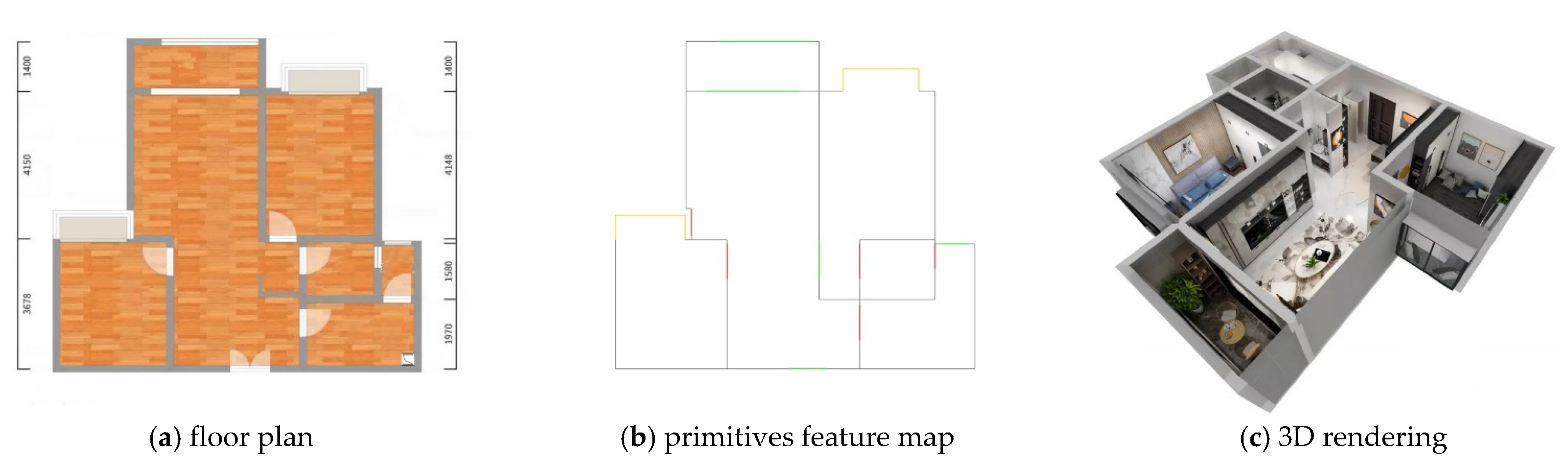
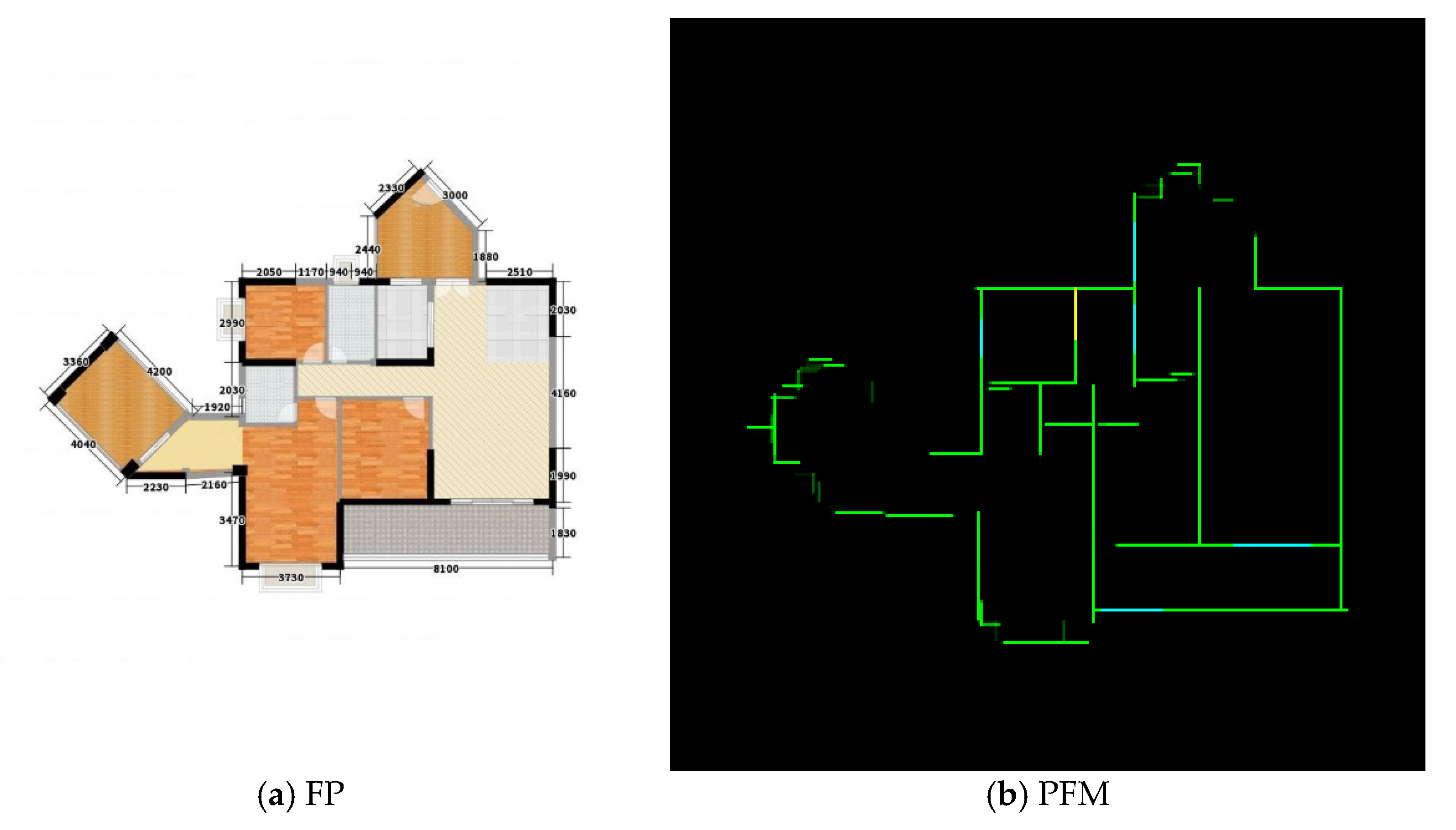
A 2D floor plan (FP) often contains structural, decorative, and functional elements and annotations. Figure 1 depicts that the vectorization of FP (VFP) aims to detect different structural primitives in the FP and assemble them into one 2D floor vector graph (FVG) that can be stretched into a 3D model. Manual methods often require meticulous measurements; thus, VFP has attracted remarkable attention for the past 20 years [1]. VFP is always a challenge because of the diversity of drawing styles and standards.
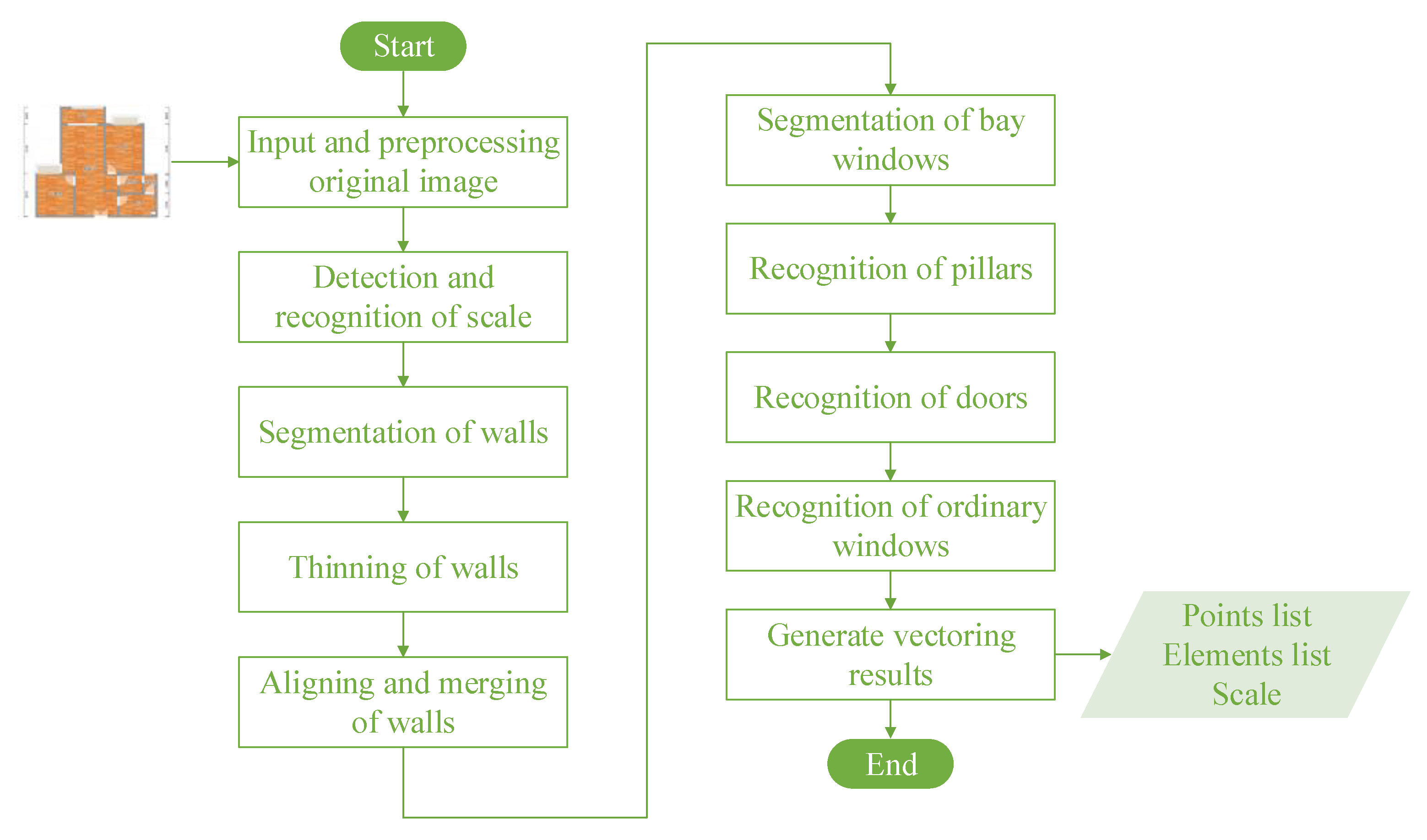
The conventional pipeline of VFP [2] (Figure 2) relies on a sequence of low-level image processing heuristics. Many researchers have devoted themselves to designing complicated algorithms to parse the local geometric constructions and retrieve structural elements based on drawing features and pixel information. Lu et al. proposed a self-incremental axis-net-based hierarchical recognition model to recognize dimensions, coordinate systems, and structural components [3], and integrate architectural information dispersed in multiple drawings and tables under the guidance of semantics and prior domain knowledge [4]. In their later work [5], the concept of primitive recognition and integration was proposed for the first time. Zhu [6] proposed a shape-operation graph to recognize walls and parse the topology of the entire layout based on structural primitives. Jiang [7] focused on the recovery of distortion to obtain the exact size. Gimenez et al. [8] also discussed methods that can be used to recognize walls, openings, and spaces. Special segmentation and recognition methods for text annotations, which could obtain high-level semantic information about scale [9], measurement [10], type of subspace [11], were proposed. The text annotations can be recognized accurately with the development of optical character recognition [12], especially those that are based on deep learning (DL) [13].
Artificial neural networks have been applied in VFP with the development of DL. Dodge et al. [14] used a fully convolutional neural network (CNN) to detect structural elements and achieve a mean intersection-over-union score of 89.9\% on R-FP and 94.4\% on the public CVC-FP dataset. Chen et al. [15] applied CNNs in translating a rasterized image to a set of junctions that represented low-level geometric and semantic information (e.g., wall corners or door endpoints). Moreover, they formulated the integer programming to aggregate junctions into a set of simple primitives (e.g., wall lines, door lines, or icon boxes) to produce an FVG with consistent constraints between topology and geometry. DL-based object detection framework can only detect doors and windows because there is no suitable annotation to describe the complex geometrical characteristic of architectural primitives. Thus, they can only replace some modules of the conventional pipeline. Faster RCNN [16] and YOLO [17], as well as other anchor-based frameworks, propose numerous boxes and combined them based on intersection over union (IoU). In a PFM, walls are described in form of lines, and if we use inflated boxes as ground truth, sloping or curved walls cannot be localized accurately. Anchor-free frameworks, CenterNet [18], and CornerNet [19] for instance, cannot solve this problem either. Subspaces segmentation is a typical semantic segmentation task, which can be achieved by a Unet [20] or a generative adversarial network (GAN) [21] in an end-to-end manner. Due to the lack of a large-scale segmentation dataset, only one literature has exploited this method on a mixed dataset PYTH [22], most samples of which are not public. Therefore, this study develops a special edge extraction GAN (EdgeGAN) to detect architectural primitives, which is a compromise between the two approaches.
GAN, which is a new learning framework for a generative model, has drawn great attention since it was proposed by Goodfellow et al. [21] in 2014. GAN has sprouted many branches, including conditional GAN [23,24], Wasserstein GAN [25,26], pix2pix [27], and has been used successfully in image translation, style migration, denoising, superresolution and repair, image matting, semantic segmentation, and dataset expansion [28,29]. GAN is a general-purpose solution for translating an input image into a corresponding output image with the same setting, which is mapped pixels to pixels.
One important milestone of GAN for image translation is pix2pix introduced by Isola et al. [27], which is developed from conditional GAN [24]. The most usual architecture of the generator is the encoder–decoder or its improved version “U-Net” with skip connections between mirrored layers in the encoder and decoder stacks [20]. Wang et al. [30] expanded pix2pix to high-resolution image synthesis and semantic manipulation by introducing a new robust adversarial learning objective together with new multiscale generator and discriminator architectures. In another work of Wang et al. [31], a video-to-video translation framework with spatial–temporal adversarial objective achieved high-resolution, photorealistic, and temporally coherent video results on a diverse set of input formats including segmentation masks, sketches, and poses.
CycleGAN is another important milestone for the unpaired image-to-image translation [32]. Two independent works also proposed the same method inspired by different motivations, namely, as DuelGAN [33] or DiscoNet [34]. Pix2pix learns the forward mapping (i.e., ), whereas CycleGAN learns two-cycle mappings (i.e., and ) with the input and output unpaired. Considering that pixel-level annotation for most tasks is impossible, CycleGAN has a wider range of applications while requiring the training of more samples.
In this work, a new VFP framework based is proposed based on pix2pix. The main contributions of this work are presented as follows:
- (1)
- A colorful and larger dataset called ZSCVFP is established. Unlike current public datasets, which only contain black and white FPs without decorative disturbance or style variation, such as CVC-FP [14] and CubiCasa5K [35], ZSCVFP’s FPs are drawn with decorative disturbance in different styles, thereby causing difficulty in the extraction of primitives. The ground truth annotations in the form of points and lines, together with the corresponding images, are provided. Furthermore, ZSCVFP has a total of 10,800 samples. This number is higher than the 121 and 5000 samples of CVC-FP and CubiCasa5K, respectively.
- (2)
- VFP is formulated as an image translation task innovatively, and EdgeGAN based on pix2pix is designed for the new task. EdgeGAN projects the FPs into the primitive space. Each channel of the primitive feature map (PFM) only contains some lines that represent one category of primitives. A self-supervising term is added to the generative loss of EdgeGAN to enhance the quality of PFM. Unlike conventional pipelines (even if some modules are replaced with deep-learning methods) that consist of a series of carefully designed algorithms, EdgeGAN obtains the FVG in an end-to-end manner. EdgeGAN is about 15 times as fast as the conventional pipeline. To the best knowledge of the authors, this study is the first to apply GAN in VFP.
- (3)
- Four criteria, which are sufficient conditions for a fully connected graph, are given to inspect the connectivity of subspaces segmented from the PFM. The connective inspection can provide auxiliary information for the designers to adjust the FVG.
- (4)
- The graph neural network (GNN) is used to predict the categories of subspaces segmented from the PFM. Given that GNN treats the adjacent matrix of the connective graph as weights directly, it can utilize global layout information and achieve higher accuracy than other common classifying methods.
2. Problem Description
In this section, the ZSCVFP dataset and the goal of the new VFP framework are introduced.
Framework Based on EdgeGAN
As mentioned, current public datasets are all black and white without decorative disturbance. However, the original FPs provided by customers in practical applications are complex and diverse. Thus, the new dataset ZSCVFP is established for this reason. ZSCVFP contains 8800 FPs in the training set and 2000 FPs in the test set. For a given FP where and are the width and height, respectively, the pseudo-annotations of walls, windows, and doors are given in the form of a point set and three line sets , , and , respectively. The elements of , , and are paired points from . The corresponding PFM is also provided in the dataset, as shown in the center subfigure of Figure 1.
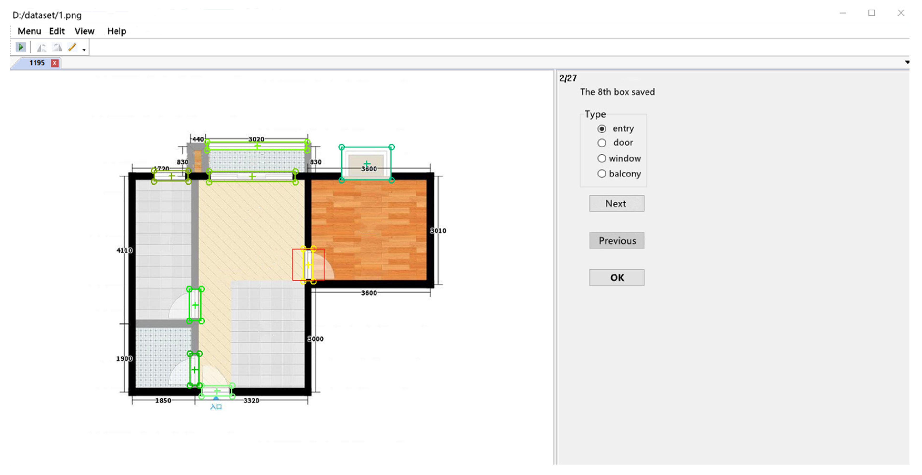
The walls’ annotations are obtained by a conventional pipeline that has been developed by ourselves in a previous work. The doors and windows are annotated manually with a tool (Figure 3). When the annotations are inconsistent, the windows and doors will be adjusted according to the walls to keep the geometrical constraints on the primitives. This adjustment will reduce the accuracy of annotations more or less.
In the new framework based on EdgeGAN, the generated PFM is denoted as where is the number of categories of primitives to be recognized. For the dataset ZSCVFP, . Each channel of is a binary image that corresponds to one primitive category. The final goal of the task, which is to extract from , is very easy if the quality of is good enough.
The set of text annotations detected in is denoted as , and the set of subspaces extracted from is denoted as . For each subspace , the feature vector consists of the number of windows, number of doors, ratio of area, etc. The feature matrix is denoted as , where is the length of the feature, is the number of subspaces. The probability matrix predicted by a GNN is denoted , where is the number of classes.
The formal representation of the new task’s goal can be summarized as follows:
- (1)
- Design a to obtain the PFM that is robust with decorative disturbances in variant styles;
- (2)
- Search for efficient criteria to inspect whether is fully connected;
- (3)
- Design a GNN to predict the category of subspaces.
3. Methods
In this section, the EdgeGAN is designed first. Then, the SCG of VFP is defined, and some connective criteria are given based on it. Lastly, a classifying GNN for subspaces is presented.
3.1. EdgeGAN
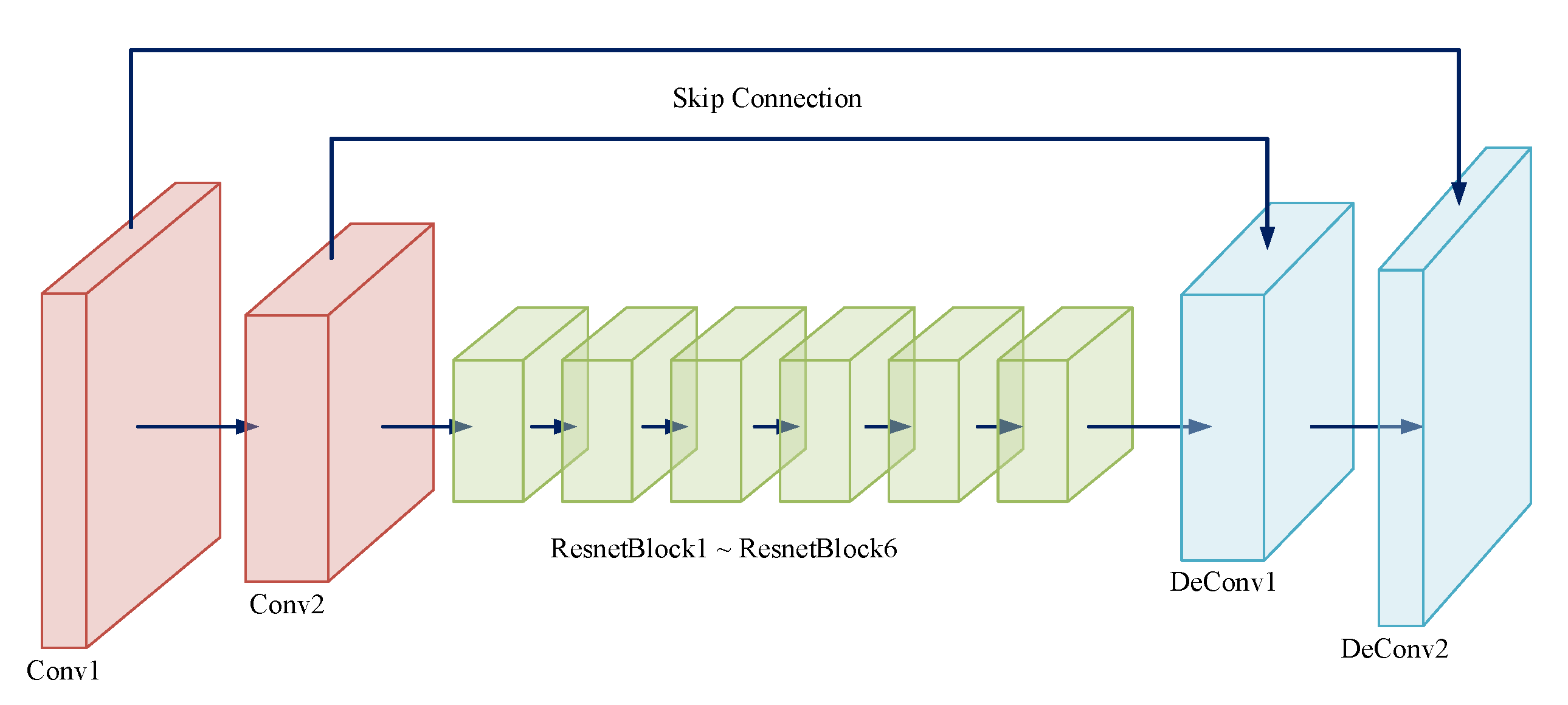
EdgeGAN learns a map from the input FPs to the output , and is the ground truth. The architecture of EdgeGAN is depicted in Figure 4. Two convolution layers, six Resnet blocks, and two deconvolution layers are connected in series with skip connect, which is a typical realization of U-Net [20] that has been used widely [27].
Two special kernels are defined as
, and .
The generative loss function of EdgeGAN is defined as
and the discriminative loss function is defined as
where is the batch size and is a filter function defined as
In the loss functions, , , and are all binary cross-entropy (BCE) loss, and are L1 loss, and and are the weights for them. Those 3 BCE terms, which constitute the standard GAN loss and are designed for the maximin optimization problem
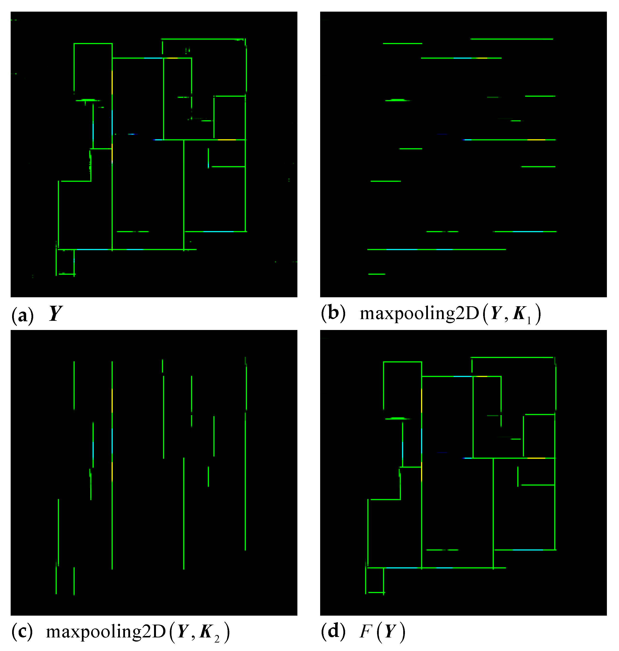
guide the generator to generate better PFM and the discriminator to recognize the difference between the distribution of and that of the ground truth . Additionally, provides pixel-level supervision information that is suitable for a pix2pix task. is a new term that composes a self-supervised loss about . In , composes a max-pooling operation with a kernel on the input multichannel image . With those two special kernels and , the can extract the horizontal and vertical lines, respectively, as illustrated in Figure 5b,c. The horizontal and vertical maps are added then. As those elements of the intersections would be bigger , we designed a clip function to truncate it. With the clip function , elements of smaller than become , and elements larger than become . The operation makes the filtered PFM still be a probability map. The adding and clipping operations combine those lines to a new PFM, in which many isolate points have been filtered, as illustrated in Figure 5d.
With the self-supervised loss, the generator will learn to generate PFMs of higher quality. As and are designed for horizontal and vertical lines, it is not going to work for irregular walls.
In each training batch, the generator and discriminator are updated alternatively. is set to 0 in the first several epochs to keep playing a leading role in the initial stage of training. When the PFM can be generated roughly, the self-supervising loss starts to come into play gradually.
3.2. Criteria for Connective Inspection
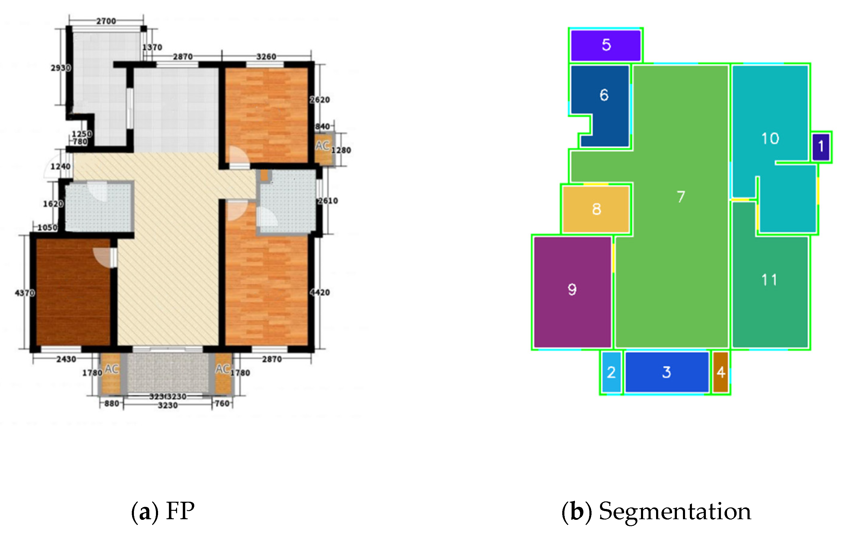
The set of subspaces extracted from a vector graph is denoted as , where are the internal subspaces, and is the subspace outside the external contour, as shown in Figure 6 and Figure 7. As the regions annotated with “AC” in Figure 6 are the spaces for air conditioners out of the door, they are ignored in Figure 7 and Figure 8. The undirected graph of can be written as , where , and . and if subspace and are connected with a door; moreover, and if subspace and are connected with a window. Denote the adjacency matrix as . The elements , , of has the following properties:
- (1)
- if ; if ; otherwise ;
- (2)
- ;
- (3)
- , that is, is symmetrical.
The subgraph without windows and its adjacency matrix are denoted as and respectively. The elements if , otherwise . The Laplacian matrix of is defined as , and its eigenvalues are denoted as . If , then is a connected graph.
The degree of internal and external connectivity of each subspace are denoted as and respectively. The criteria for inspection of connectivity include the following:
- (1)
- There is a door on the external door at least, i.e., ;
- (2)
- The number of doors on the external doors is often less than 2, i.e., ;
- (3)
- Each subspace except those with special architectural functionality (for example, the regions for air condition and pipe) has at least one door, that is, and , where ;
- (4)
- is a connected graph, that is, .
All those four criteria are sufficient conditions for a fully connected graph. Furthermore, Criterion (4) is the sufficient condition of Criteria (1)–(3), but its computation is much complicated than other criteria.
3.3. Classifying of Subspaces Based on GNN
A GNN with layers is defined as
where is the index of layer, is the weight parameters to be learned, is the output dimension of the th layer of the GNN, and is the activation function.
The input of GNN is the feature matrix of and the output is the classifying probability matrix , where is the length of the feature, is the number of subspaces, and is the number of categories. The input dimension of the first layer is , and the last output is with .
The BCE loss function adopted to train the GNN is as follows:
where is the one-hot labeled category. Considering that the number of subspaces in each VFP varies, is expanded to with , and is expanded to with . The output dimension of the last layer becomes and the label vector . The labels of subspace are coded from 0 to . Thus, the new virtual subspace is labeled with .
4. Experimental Results and Discussion
In this section, three experiments are conducted to illustrate the proposed methods. First, EdgeGAN is compared with the DL-based pipeline on the ZSCCSVFP dataset. Second, the usage of connective criteria is demonstrated by presenting an example. Lastly, the GNN is compared with four common classifying methods to validate its advantage in terms of structural information.
4.1. EdgeGAN
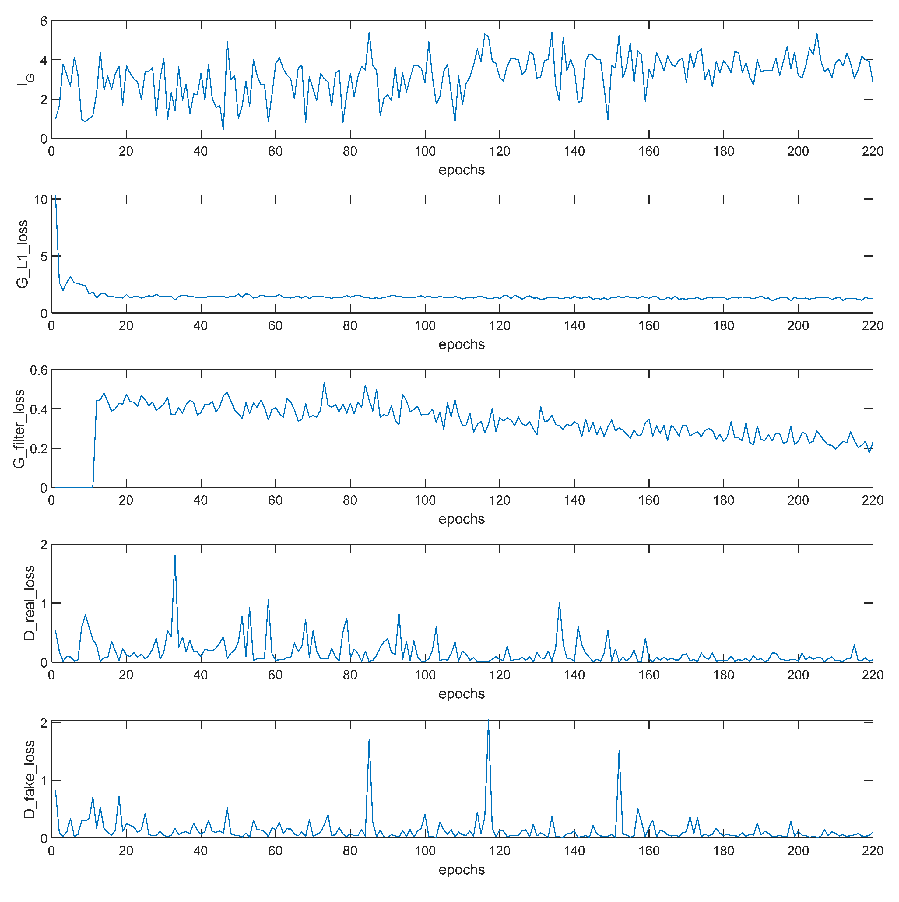
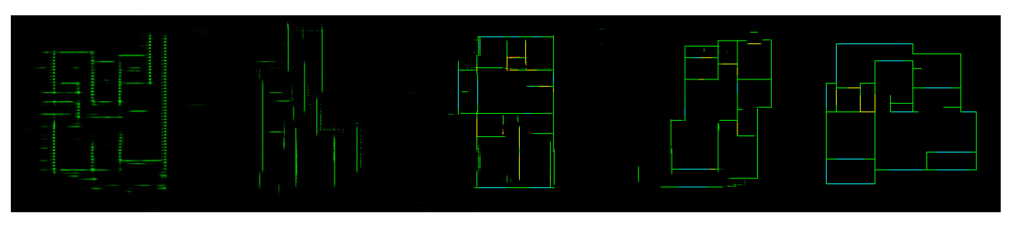
In this experiment, all training sets are executed on the hardware platform “CPU Intel Core i9-9900K, 64 GB memory, and GPU NVIDIA RTX2080TI×2,” and the software is “Python 3.6, Pytorch 1.4.0 [36], Cuda 10.0, and Cudnn 7.4.2 [37].” The maximal training epoch is 220, and the batch size is 128. is always set to 10, and is set to 0 in the first 10 epochs and 100 in the subsequent epochs. The learning rate is set to 0.0002 at the first 20 epochs and decreased to 0 linearly in subsequent epochs. The training is recorded in Figure 8. is 0 in the first 10 epochs and decreases gradually. The is stable at approximately 1.38 since the 20th epoch. Thus, it is not a suitable measurement of accuracy. The corresponding evolutionary process of is depicted in Figure 9.
The quality of generated images can be divided into three levels:
- (1)
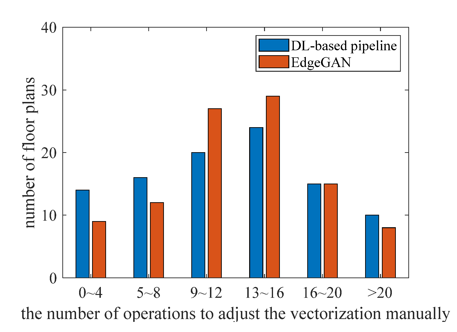
- Level 1: The generated images are free from noisy points and have high-quality lines, and the recognition accuracy of primitives is close to the conventional pipeline. The proportion of level 1 is approximately 40%. These images can be used to obtain vector graphics with a few manual adjustments, similar to the conventional pipeline. Figure 10 compares the number of adjusting operations that are counted by a decoration designer on 100 FPs with level 1 results. Although the results of EdgeGAN satisfy the requirements of the application, its performance is still slightly weaker than that of the DL-based pipeline. The mean value of operations of the DL-based pipeline (16.50) is close to that of EdgeGAN (16.67). However, the standard deviation of EdgeGAN (8.34) is much larger than that of the DL-based pipeline (4.4628), which means that the latter is more stable. Moreover, 30 PFMs generated by the DL-based pipeline need less than eight operations, while only 21 PFMs by EdgeGAN, which means that the former has a higher rate of excellence. The results of EdgeGAN. Considering that the pseudo-ground truth annotations themselves are obtained on the basis of the conventional pipeline and suffer from inaccuracy, the results are reasonable. The performance of EdgeGAN can be improved if it is training on a larger and higher quality dataset.
- (2)
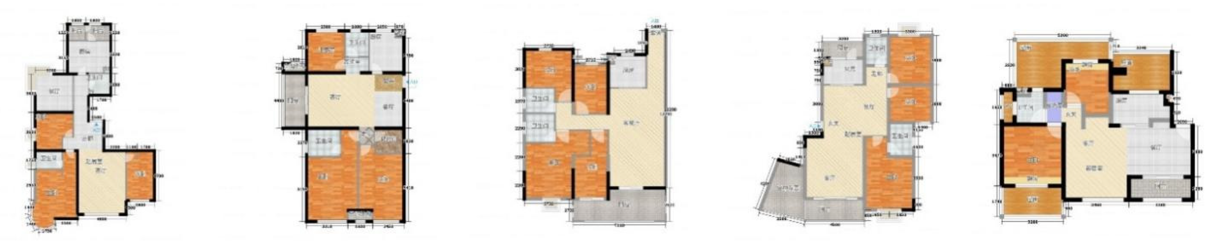
- Level 2: In addition to inaccurate primitives, some noisy points, broken lines, redundancy lines, or unaligned lines are presented in the generated images, as shown in the lines in the main body of Figure 11. The proportion of level 2 is approximately 55%. The self-supervising loss can relieve but cannot eliminate this phenomenon. Some postprocessing methods are necessary to address these problems. Solving this problem by using the EdgeGAN itself is direct but still challenging.
- (3)
- Level 3: Serious defects in quality or accuracy with a proportion of approximately 5% are observed in the sloping walls in Figure 11. The reason is that the number of samples with sloping walls is less than 100, which is much less than horizontal and vertical walls.
On one single RTX2080TI, the frame rate of EdgeGAN and its postprocessing is approximately 32 fps; and the frame of the DL-based pipeline on an Intel 9900 K CPU is approximately 2 fps. Although EdgeGAN can obtain PFM at a much higher speed, a gap still exists between the integral accuracy and quality of generated images and the requirements of applications.
4.2. Connectivity of Subspaces
The adjacent matrix of the vector graph in Figure 6 is as follows. Notably, subspace 1, 2, and 4 are ignored.
Thus, the Laplacian matrix is
The graph is not connected because . shows that the presence of five unconnected loops. Other criteria can also be calculated easily with .
4.3. Classifying of Subspaces Based on GNN
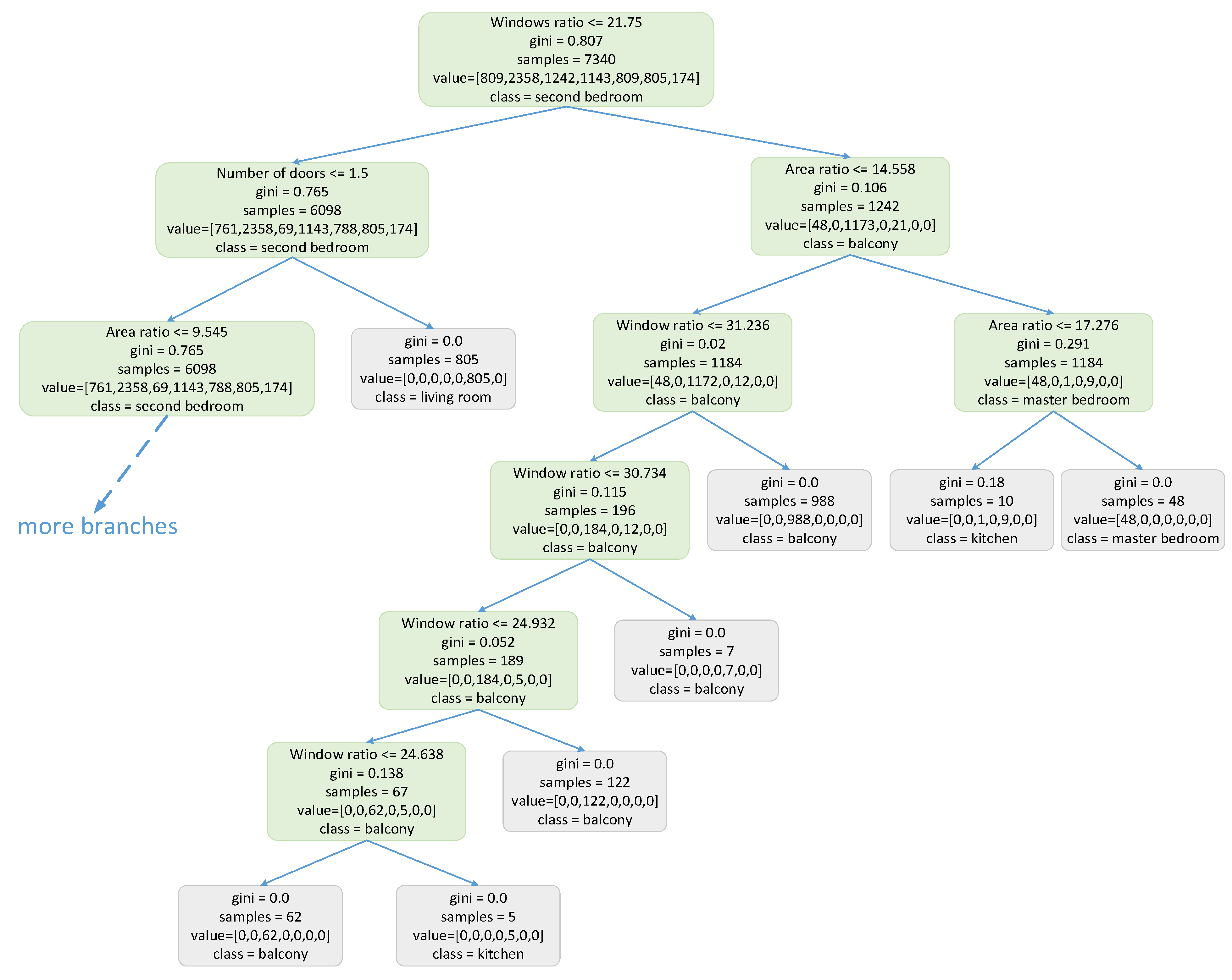
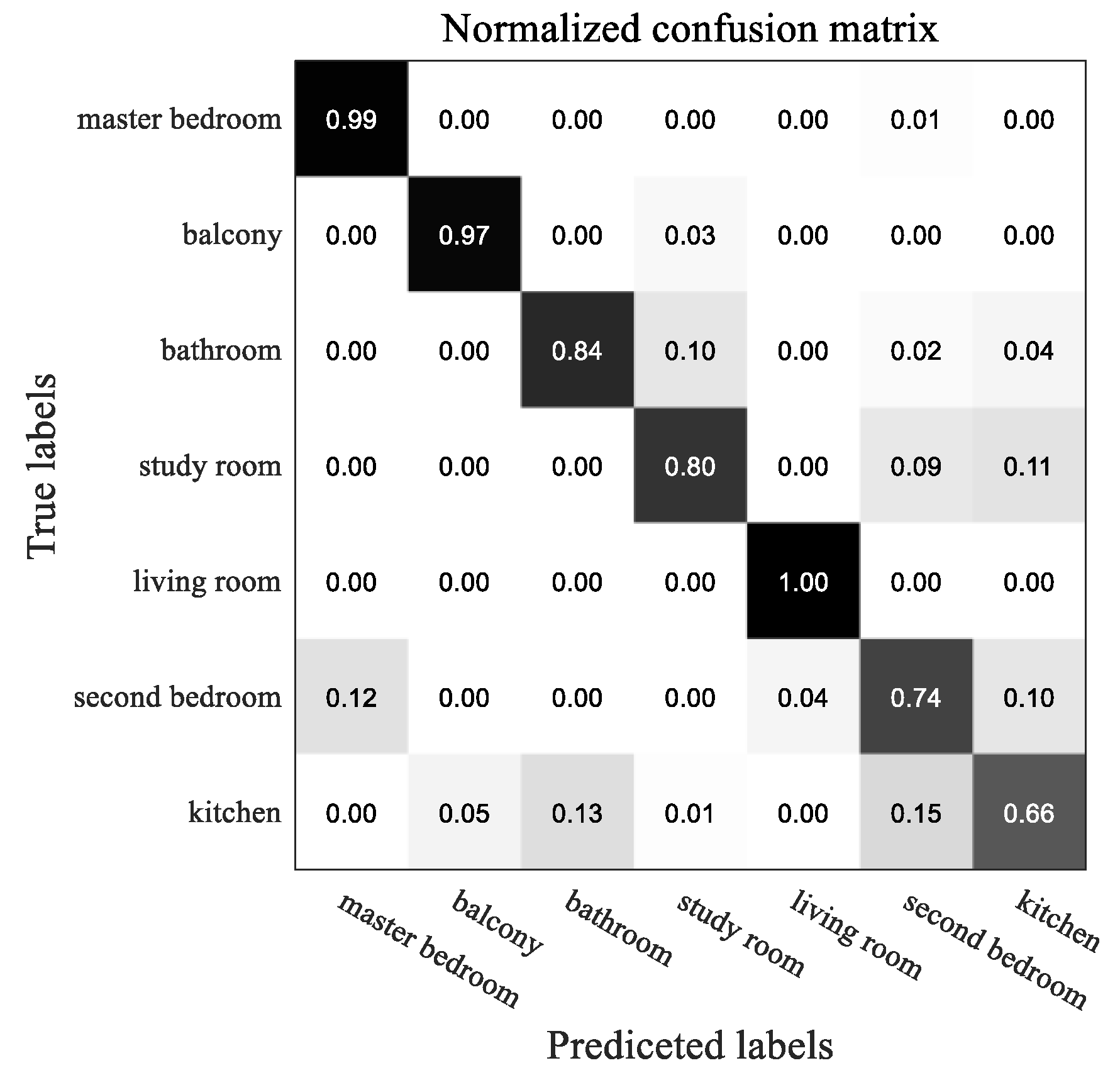
A new dataset that contains feature matrices annotated with subspace types is established to validate the advantage of GNN. The distributions of instances in the dataset are listed in Table 1. The features used here include window ratio, area ratio, number of doors, number of windows, and number of edges. Four widely used methods [38], namely, C4.5, iterative dichotomiser 3 (ID3), basic backpropagation (BP) neural network, and classification and regression tree (CART), are compared with GNN. The input of these four methods is the feature vector of one subspace, which means that they can only predict the type of one subspace independently. The input dimension of the BP network with one hidden layer is 5, the output dimension is 7, and the number of neurons in the hidden layer is 20. Part of the decision tree obtained by CART is shown in Figure 12.
5. Conclusions
EdgeGAN generates PFM in an end-to-end manner with a frame rate of 32 fps on an RTX2080TI GPU, which is much faster than the DL-based pipeline’s 2 fps since many modules of the pipeline can only run on a CPU. Although the accuracy of EdgeGAN is slightly lower than that of the DL-based pipeline, especially on sloping walls, its potential can be further exploited if given a larger and higher quality training set. Four connective criteria are proposed to inspect the connectivity of subspaces segmented from one FP. Those criteria are also suitable for postprocessing the results of traditional methods and object detection frameworks. GNN utilizes the connective information to predict the categories of subspaces and achieves 4.69% higher accuracy than other classification approaches. The category information of subspaces can be used to check with the depictive texts of FP.
In this study, since the PFM generation and subspace segmentation are fulfilled separately, the computing speed and performance can be improved further if they are realized in an end-to-end manner based on a one-stage framework. Thus, we will develop a one-stage multitask framework that finishes primitive detection, subspace segmentation, optical character recognition, and consistency inspection, simultaneously, in a future study. Furthermore, to improve the quality of PFM about irregular walls, some deep activate contour methods, such as deep snake [39] and deep level set loss [40], will also be exploited.
Author Contributions
Conceptualization, data curation, K.Z.; methodology, S.D.; project administration, W.L.; software, W.W. All authors have read and agreed to the published version of the manuscript.
Funding
This work is supported by the Guangdong Basic and Applied Basic Research Projects (2019A1515111082, 2020A1515110504), Fund for High-Level Talents Afforded by University of Electronic Science and Technology of China, Zhongshan Institute (417YKQ12, 419YKQN15), Social Welfare Major Project of Zhongshan (2019B2010, 2019B2011), Achievement Cultivation Project of Zhongshan Industrial Technology Research Institute (419N26), and Young Innovative Talents Project of Education Department of Guangdong Province (419YIY04).
Institutional Review Board Statement
Not applicable.
Informed Consent Statement
Not applicable.
Conflicts of Interest
The authors declare no conflict of interest.
Abbreviations
All abbreviations notations used in this work are listed below.
| FP | floor plans |
| VFP | vectorization of floor plans |
| FVG | floor vector graph |
| PFM | primitive feature map |
| SCG | subspace connective graph |
| GAN | generative adversarial network |
| GNN | graph neural network |
| EdgeGAN | edge extraction GAN |
| ZSCVFP | private dataset established by us |
References
- Lewis, R.; Séquin, C. Generation of 3D building models from 2D architectural plans. Comput. Aided Des. 1998, 30, 765–779. [Google Scholar] [CrossRef]
- Gimenez, L.; Hippolyte, J.-L.; Robert, S.; Suard, F.; Zreik, K. Review: Reconstruction of 3D building information models from 2D scanned plans. J. Build. Eng. 2015, 2, 24–35. [Google Scholar] [CrossRef]
- Lu, T.; Tai, C.-L.; Su, F.; Cai, S. A new recognition model for electronic architectural drawings. Comput. Aided Des. 2005, 37, 1053–1069. [Google Scholar] [CrossRef]
- Lu, T.; Tai, C.-L.; Bao, L.; Su, F.; Cai, S. 3D Reconstruction of Detailed Buildings from Architectural Drawings. Comput. Aided Des. Appl. 2005, 2, 527–536. [Google Scholar] [CrossRef]
- Lu, T.; Yang, H.; Yang, R.; Cai, S. Automatic analysis and integration of architectural drawings. Int. J. Doc. Anal. Recognit. 2006, 9, 31–47. [Google Scholar] [CrossRef]
- Zhu, J. Research on 3D Building Reconstruction from 2D Vector Floor Plan Based on Structural Components Recognition. Master’s Thesis, Tsinghua University, Beijing, China, 2013. [Google Scholar]
- Jiang, Z. Research on Floorplan Image Recognition Based on Shape and Edge Features. Master’s Thesis, Harbin Institute of Technology, Harbin, China, 2016. [Google Scholar]
- Gimenez, L.; Robert, S.; Suard, F.; Zreik, K. Automatic reconstruction of 3D building models from scanned 2D floor plans. Autom. Constr. 2016, 63, 48–56. [Google Scholar] [CrossRef]
- Tombre, K.; Tabbone, S.; Pelissier, L.; Lamiroy, B.; Dosch, P. Text/Graphics Separation Revisited. In International Workshop on Document Analysis Systems; Springer: Berlin/Heidelberg, Germany, 2002; pp. 200–211. [Google Scholar]
- Ahmed, S.; Weber, M.; Liwicki, M.; Dengel, A. Text/Graphics Segmentation in Architectural Floor Plans. In Proceedings of the 2011 International Conference on Document Analysis and Recognition, Beijing, China, 18–21 September 2011; pp. 734–738. [Google Scholar]
- Ahmed, S.; Liwicki, M.; Weber, M.; Dengel, A. Automatic Room Detection and Room Labeling from Architectural Floor Plans. In Proceedings of the 10th IAPR International Workshop on Document Analysis Systems, Gold Coast, Australia, 27–29 March 2012; pp. 339–343. [Google Scholar]
- Smith, R. An overview of the Tesseract OCR engine. In Proceedings of the Ninth International Conference on Document Analysis and Recognition (ICDAR 2007), Curitiba, Brazil, 23–26 September 2007; Volume 2, pp. 629–633. [Google Scholar]
- Long, S.; He, X.; Yao, C. Scene Text Detection and Recognition: The Deep Learning Era. Int. J. Comput. Vis. 2021, 129, 161–184. [Google Scholar] [CrossRef]
- Dodge, S.; Xu, J.; Stenger, B. Parsing floor plan images. In Proceedings of the 2017 Fifteenth IAPR International Conference on Machine Vision Applications (MVA), Nagoya, Japan, 8–12 May 2017; pp. 358–361. [Google Scholar]
- Liu, C.; Wu, J.; Kohli, P.; Furukawa, Y. Raster-to-Vector: Revisiting Floorplan Transformation. In Proceedings of the 2017 IEEE International Conference on Computer Vision (ICCV), Venice, Italy, 22–29 October 2017; pp. 2214–2222. [Google Scholar]
- Ren, S.; He, K.; Girshick, R.; Jian, S. Faster R-CNN: Towards Real-Time Object Detection with Region Proposal Networks. IEEE Trans. Pattern Anal. Mach. Intell. 2015, 39, 1137–1149. [Google Scholar] [CrossRef] [Green Version]
- Bochkovskiy, A.; Wang, C.-Y.; Liao, H.-Y.M. YOLOv4: Optimal Speed and Accuracy of Object Detection. arXiv 2020, arXiv:2004.10934v1. [Google Scholar]
- Duan, K.; Bai, S.; Xie, L.; Qi, H.; Huang, Q.; Tian, Q. CenterNet: Object Detection with Keypoint Triplets. arXiv 2019, arXiv:1904.08189v1. [Google Scholar]
- Law, H.; Deng, J. CornerNet: Detecting Objects as Paired Keypoints. arXiv 2019, arXiv:1808.01244v2. [Google Scholar]
- Ronneberger, O.; Fischer, P.; Brox, T. U-net: Convolutional networks for biomedical image segmentation. In Proceedings of the International Conference on Medical Image Computing and Computer-Assisted Intervention, Cham, Switzerland, 5–9 October 2015; pp. 234–241. [Google Scholar]
- Goodfellow, I.J.; Pouget-abadie, J.; Mirza, M.; Xu, B.; Warde-farley, D. Generative Adversarial Nets. arXiv 2014, arXiv:1406.2661v1. [Google Scholar]
- Sandelin, F. Semantic and Instance Segmentation of Room Features in Floor Plans Using Mask R-CNN. Master’s Thesis, Uppsala University, Uppsala, Sweden, 2019. [Google Scholar]
- Mirza, M.; Osindero, S. Conditional Generative Adversarial Nets. arXiv 2014, arXiv:1411.1784v1. [Google Scholar]
- Odena, A.; Olah, C.; Shlens, J. Conditional Image Synthesis with Auxiliary Classifier GANs. In Proceedings of the International Conference on Machine Learning, ICML 2017, Sydney, Australia, 6–11 August 2017; Volume 6, pp. 4043–4055. [Google Scholar]
- Arjovsky, M.; Chintala, S.; Bottou, L. Wasserstein GAN. arXiv 2017, arXiv:1701.07875v3. [Google Scholar]
- Gulrajani, I.; Ahmed, F.; Arjovsky, M.; Dumoulin, V.; Courville, A. Improved Training of Wasserstein GANs. arXiv 2017, arXiv:1704.00028v3. [Google Scholar]
- Isola, P.; Zhu, J.-Y.; Zhou, T.; Efros, A.A. Image-to-Image Translation with Conditional Adversarial Networks. In Proceedings of the IEEE Conference on Computer Vision and Pattern Recognition, Honolulu, HI, USA, 21–26 July 2017; pp. 5967–5976. [Google Scholar]
- Creswell, A.; White, T.; Dumoulin, V.; Arulkumaran, K.; Sengupta, B.; Bharath, A.A. Generative Adversarial Networks: An Overview. IEEE Signal Process. Mag. 2018, 35, 53–65. [Google Scholar] [CrossRef] [Green Version]
- Hong, Y.; Hwang, U.; Yoo, J.; Yoon, S. How Generative Adversarial Networks and Their Variants Work. ACM Comput. Surv. 2019, 52, 1–43. [Google Scholar] [CrossRef] [Green Version]
- Wang, T.C.; Liu, M.Y.; Zhu, J.Y.; Tao, A.; Kautz, J.; Catanzaro, B. High-Resolution Image Synthesis and Semantic Manipulation with Conditional GANs. In Proceedings of the IEEE International Conference on Computer Vision (ICCV), Venice, Italy, 22–29 October 2017; pp. 8798–8807. [Google Scholar]
- Wang, T.; Liu, M.; Zhu, J.; Liu, G.; Tao, A.; Kautz, J.; Catanzaro, B. Video-to-Video Synthesis. arXiv 2018, arXiv:1808.06601v2. [Google Scholar]
- Zhu, J.-Y.; Park, T.; Isola, P.; Efros, A.A. Unpaired Image-to-Image Translation Using Cycle-Consistent Adversarial Networks. In Proceedings of the 2017 IEEE International Conference on Computer Vision (ICCV), Venice, Italy, 22–29 October 2017; pp. 2242–2251. [Google Scholar]
- Yi, Z.; Zhang, H.; Tan, P.; Gong, M. DualGAN: Unsupervised Dual Learning for Image-to-Image Translation. In Proceedings of the 2017 IEEE International Conference on Computer Vision (ICCV), Venice, Italy, 22–29 October 2017; pp. 2868–2876. [Google Scholar]
- Kim, T.; Cha, M.; Kim, H.; Kwon, J.; Jiwon, L. Learning to Discover Cross-Domain Relations with Generative Adversarial Networks. arXiv 2017, arXiv:1703.05192. [Google Scholar]
- Kalervo, A.; Ylioinas, J.; Häikiö, M.; Karhu, A.; Kannala, J. CubiCasa5K: A Dataset and an Improved Multi-task Model for Floorplan Image Analysis. arXiv 2019, arXiv:1904.01920. [Google Scholar]
- Facebook. Available online: https://Pytorch.Org/ (accessed on 13 October 2020).
- Nvidia. Available online: https://Developer.Nvidia.Com/Zh-Cn/Cuda-Toolkit (accessed on 25 June 2020).
- Li, H. Statistical Learning Method; Tsinghua Press: Beijing, China, 2019. [Google Scholar]
- Zambaldi, V.; Raposo, D.; Santoro, A.; Bapst, V. Relational Deep Reinforcement Learning. arXiv 2018, arXiv:1806.01830v2. [Google Scholar]
- Kim, Y.; Kim, S.; Kim, T.; Kim, C. CNN-Based Semantic Segmentation Using Level Set Loss. In Proceedings of the 2019 IEEE Winter Conference on Applications of Computer Vision (WACV), Waikoloa Village, HI, USA, 8–10 January 2019; pp. 1752–1760. [Google Scholar]
Figure 1.
Reconstructing the 3D model from a 2D floor plan.

Figure 2.
Conventional pipeline of VFP.

Figure 3.
The annotation tool for primitives.

Figure 4.
Architecture of EdgeGAN.

Figure 5.
The self-supervising filter of EdgeGAN.

Figure 6.
Segmentation of FP.

Figure 7.
Subspace connective graph.

Figure 8.
The curve of loss.

Figure 9.
Generated images in epoch 10, 60, 110, 160, 210.


Figure 10.
Comparison between conventional pipeline and EdgeGAN.

Figure 11.
The undetected sloping walls.

Figure 12.
Decision tree of CART.

Figure 13.
Confusion matrix of CART.

Figure 14.
Confusion matrix of GNN.


Table 1.
Number of instances in the dataset.
| Training Set | Test Set | |
|---|---|---|
| master bedroom | 809 | 200 |
| balcony | 1242 | 315 |
| bathroom | 1143 | 287 |
| study room | 174 | 46 |
| living room | 809 | 200 |
| second bedroom | 2358 | 587 |
| kitchen | 805 | 200 |
Table 2.
Accuracy of subspace decision.
| Method | C4.5 | ID3 | BP | CART | GNN |
|---|---|---|---|---|---|
| Accuracy | 74.82% | 75.49% | 79.13% | 79.66% | 84.35% |
Publisher’s Note: MDPI stays neutral with regard to jurisdictional claims in published maps and institutional affiliations. |
© 2021 by the authors. Licensee MDPI, Basel, Switzerland. This article is an open access article distributed under the terms and conditions of the Creative Commons Attribution (CC BY) license (https://creativecommons.org/licenses/by/4.0/).
Share and Cite
MDPI and ACS Style
Dong, S.; Wang, W.; Li, W.; Zou, K. Vectorization of Floor Plans Based on EdgeGAN. Information 2021, 12, 206. https://0-doi-org.brum.beds.ac.uk/10.3390/info12050206
AMA Style
Dong S, Wang W, Li W, Zou K. Vectorization of Floor Plans Based on EdgeGAN. Information. 2021; 12(5):206. https://0-doi-org.brum.beds.ac.uk/10.3390/info12050206
Chicago/Turabian StyleDong, Shuai, Wei Wang, Wensheng Li, and Kun Zou. 2021. "Vectorization of Floor Plans Based on EdgeGAN" Information 12, no. 5: 206. https://0-doi-org.brum.beds.ac.uk/10.3390/info12050206
Note that from the first issue of 2016, this journal uses article numbers instead of page numbers. See further details here.