A Survey on Old and New Approximations to the Function ϕ(x) Involved in LDPC Codes Density Evolution Analysis Using a Gaussian Approximation

Abstract

Low Density Parity Check (LDPC) codes are currently being deeply analyzed through algorithms that require the capability of addressing their iterative decoding convergence performance. Since it has been observed that the probability distribution function of the decoder’s log-likelihood ratio messages is roughly Gaussian, a multiplicity of moderate entanglement strategies to this analysis has been suggested. The first of them was proposed in Chung et al.’s 2001 paper, where the recurrent sequence, characterizing the passage of messages between variable and check nodes, concerns the function $\varphi \left(x\right)$, therein specified, and its inverse. In this paper, we review this old approximation to the function $\varphi \left(x\right)$, one variant on it obtained in the same period (proposed in Ha et al.’s 2004 paper), and some new ones, recently published in two 2019 papers by Vatta et al. The objective of this review is to analyze the differences among them and their characteristics in terms of accuracy and computational complexity. In particular, the explicitly invertible, not piecewise defined approximation of the function $\varphi \left(x\right)$, published in the second of the two abovementioned 2019 papers, is shown to have less relative error in any x than most of the other approximations. Moreover, its use conducts to an important complexity reduction, and allows better Gaussian approximated thresholds to be obtained.

1. Introduction

The investigation of Low Density Parity Check (LDPC) codes decoding, carried out by means of the belief propagation algorithm, usually takes place by analyzing the evolution of the probability densities of the messages exchanged between check and variable nodes of the bipartite (Tanner) graph describing a code belonging to this family [1]. However, this is a rather complicated job due to the continuous nature of the messages themselves, which makes them difficult to analyze. To avoid the difficulty of this task, Chung et al. presented, in [2], a Gaussian approximation (GA) (Despite its limits (see, e.g., [3,4]), the use of the GA is very convenient when a powerful and effortless approach is required. See its recent adoption, e.g., to obtain “bounds on LDPC decoding thresholds [5], rate-compatible puncturing patterns for LDPC codes [6,7], analytical bit-error rate (BER) expressions [8], and unequal error protection (UEP) LDPC codes [9].”) for the message probability distribution, simplifying the evolution of the infinite dimensional density space to the evolution of a single parameter. They mathematically described the passage of messages between variable and check nodes of the Tanner graph by means of a recurring succession of the mean values of the check nodes’ output messages, having shown that regular LDPC codes present message densities that are roughly Gaussian, whereas irregular ones present message densities that are Gaussian combinations [10]. In this way, instead of describing the variable and check node output message as a function of the incoming messages from their respective neighbors, a recursive sequence is obtained by expressing a check node output message mean value at the l-th iteration as a function of the same mean value at the $(l-1)$-th iteration [4]. The belief-propagation decoding thresholds, also known as density evolution thresholds—addressing LDPC codes iterative decoding convergence performance and defined as the maximum channel noise level such that the probability of error of the belief-propagation decoding algorithm tends to zero as the number of its iterations tends to infinity [2]—may be approximated by evaluating the last value of the channel noise variance ${\sigma }_n^2$ such that this recurrent sequence converges, or, equivalently, as the first ${\sigma }_n^2$ value such that the sequence diverges, obtaining the so-called GA thresholds.

The recurrent sequence in [2] is expressed through the function $\varphi \left(x\right)$, defined in the aforementioned paper. Its study has been performed in [3], to obtain tighter upper and lower bounds on it for $x>0$. Chung et al.’s lower and upper bounds $(1-3/x)\psi \left(x\right)$ and $(1+1/7x)\psi \left(x\right)$ with $\psi \left(x\right)=\sqrt{\pi /x}exp(-x/4)$, holding for the function $\varphi \left(x\right)$ involved in the GA, have been both analytically proved in [3] to be improved by replacing 3 with ${\pi }^2/4$ and $1/7x$ with 0, respectively. It was shown in [3] that the tighter upper bound therein obtained is explicitly invertible through the Lambert $W$-function (also called omega function or product logarithm), whereas the one obtained in [2] is not explicitly invertible. Moreover, on the basis of the two tighter bounds on $\varphi \left(x\right)$ found, a piecewise defined approximation of $\varphi \left(x\right)$ has been obtained in [3]. This is analogous but improved with respect to the one in [2], in the sense that it allows to obtain GA thresholds closer to the ones obtained applying density evolution than the GA thresholds given in [2]. In [10], a new approximation of the function $\varphi \left(x\right)$ was given, which, unlike the other approximations found in the literature (see [2,3,6]),

• is not piecewise defined in the definition interval $[0,+\infty [$ i.e., it is defined through a unique mathematical expression,
• is explicitly invertible,
• remains between the two above said tighter bounds of [3] in the domain of interest,
• and has less relative error for any value of x than most of the other approximations, when the error is evaluated by computing $\varphi \left(x\right)$ numerically through a Mathematica^® statement published in [11].

As noted in [10], the fact that this new approximation has always an univocal analytical expression (i.e., it is not piecewise defined) implies its easy mathematical handling, in contrast to formerly defined piecewise functions, defined by distinct analytical expressions being dependent on the range of values taken by the argument x. Moreover, its explicit invertibility implies that no interpolated functions approximating it by points $(x_k,\varphi \left(x_k\right))$ and its inverse by points $(\varphi \left(x_k\right),x_k)$ are required. These properties conduct to an important complexity reduction of the algebraic handling and utilization of the approximation itself. Moreover, its use allows better GA thresholds to be obtained, in the sense that they approximate the thresholds obtained with density evolution better than the GA thresholds obtained in [2].

In this paper, a review of the abovementioned old approximations (published in [2,6]) and new approximations (published in [3,10]) to the function $\varphi \left(x\right)$ is performed, so that to analyze the differences among them and their characteristics in terms of accuracy and computational complexity. The paper is organized as follows. In the next section, we review the GA for irregular LDPC code density evolution. Section 3 is dedicated to the valuable merits an approximation should have: among them, there is the explicit invertibility, addressed in Section 6. Section 4 recalls the definitions of absolute and relative errors as means to evaluate the accuracy of an approximation. Section 5 recalls the function $\varphi \left(x\right)$ specified in [2] and the literature where its principal approximations were presented. Section 6 addresses the approximation of the inverse ${\varphi }^{-1}\left(y\right)$. Section 7 compares the numerical results-in terms of calculated GA thresholds-obtained applying the approximations to $\varphi \left(x\right)$ reviewed in the paper, and, finally, Section 8 recapitulates the conclusions.

2. Gaussian Approximation for Irregular LDPC Codes

We treat irregular LDPC codes as it has been shown that they behave better than regular ones [12]. Furthermore, it was shown in [2] and recalled in [10] that message densities are roughly Gaussians for regular LDPC codes or Gaussian mixtures for irregular ones, and hence regular LDPC codes can be considered as a special case of irregular ones.

Irregular LDPC codes [12] are defined by means of the distribution of the node degrees in their Tanner graphs [1], specified through the polynomials $\lambda \left(x\right)$ and $\rho \left(x\right)$ [13]:

$$\lambda \left(x\right)=\sum _{i=2}^{d_l}{\lambda }_i{x}^{i-1},$$

(1)

$$\rho \left(x\right)=\sum _{j=2}^{d_r}{\rho }_j{x}^{j-1}.$$

(2)

The $(d_l-1)$-tuple $\left\{{\lambda }_i\right\}$ and $(d_r-1)$-tuple $\left\{{\rho }_j\right\}$ both add up to 1 [14], and ${\lambda }_i$ (respectively, ${\rho }_j$) specifies the fraction of total edges in the Tanner graph insisting on a degree-i variable node (respectively, on a degree-j check node).

Express with v the output message of a variable node and with u the output message of a check node (In soft-decision belief-propagation decoding, the messages are the log-likelihood ratios (LLRs) of received bits). The first is expressed as

$$v=\log \left(\frac{P\left\{y\right|x=+1\}}{P\left\{y\right|x=-1\}}\right),$$

where x is the node bit value, and y is all the information at this node’s disposal up to the current iteration. The edge bringing the information related to v is not considered. Likewise, u is expressed as

$$u=\log \left(\frac{P\left\{y^{\prime }\right|x^{\prime }=+1\}}{P\left\{y^{\prime }\right|x^{\prime }=-1\}}\right),$$

where $x^{\prime }$ is the variable node bit value, and $y^{\prime }$ is the information at this check node’s disposal up to the current iteration, ignoring the edge bearing u [7].

Following the analysis in [2], where a one-dimensional quantity, i.e., the mean of Gaussian densities, was demonstrated to perform as a reliable replacement for the message densities themselves, we hypothesize, as in [10], that we can approximate as Gaussian the LDPC message distributions for additive white Gaussian noise (AWGN) channels and denote with $m_u^{\left(l\right)}$ and $m_v^{\left(l\right)}$ the means of u and v at the l-th iteration, respectively. Moreover, we assume the log-likelihood ratio (LLR) message $u_0$ from the channel to be Gaussian with mean $m_{u_0}=2/{\sigma }_n^2$ and variance $4/{\sigma }_n^2$, being ${\sigma }_n^2$ the variance of the channel noise. For a degree-i variable node at the lth iteration, the mean of the output yields

$$m_{v,i}^{\left(l\right)}=m_{u_0}+(i-1)m_u^{(l-1)},$$

where $m_u^{(l-1)}$ is the mean of u at the $(l-1)$-th iteration. Assuming that the codeword length tends to infinity, and consequently adducing a cycle-free Tanner graph argument, for a check node at the lth iteration, the mean of the output yields

$$m_u^{\left(l\right)}=\sum _{j=2}^{d_r}{\rho }_j{\varphi }^{-1}(1-{[1-\sum _{i=2}^{d_l}{\lambda }_i\varphi (m_{u_0}+(i-1)m_u^{(l-1)})]}^{j-1})$$

(3)

being the fundamental function $\varphi \left(x\right)$ of [2] defined as:

$$\varphi \left(x\right)=\{\begin{array}{cc}1-\frac{1}{\sqrt{4\pi x}}{\int }_{I\mathbb{R}}\tanh \frac{u}{2}{e}^{-\frac{{(u-x)}^2}{4x}}\mathrm{d}u\hfill & \mathrm{if}x>0\hfill \\ 1\hfill & \mathrm{if}x=0.\hfill \end{array}$$

(4)

Assuming $s:=m_{u_0}$ and $t_l:=m_u^{\left(l\right)}$, and defining, as in [5],

$$g_s\left(t\right)=\sum _{j=2}^{d_r}{\rho }_j{g}_{s,j}\left(t\right),$$

(5)

where

$$g_{s,j}\left(t\right)={\varphi }^{-1}(1-{[1-\sum _{i=2}^{d_l}{\lambda }_i\varphi (s+(i-1)t)]}^{j-1}),$$

(6)

the sequence (3) may be rewritten as

$$t_l=g_s\left(t_{l-1}\right).$$

(7)

Using the algorithmic method presented in [15], instead of looking for, as done in the original paper [2], the minimum value of the parameter s guaranteeing the convergence of the sequence (7), as in [10] we make use of a standard software to solve a problem of quadratic degeneracy [16]. Namely, when the second derivative $g_s^{″}\left(t\right)\ne 0$, the problem of quadratic degeneracy is the solution of the system of equations

$$\left\{\begin{array}{c}{g}_s\left(t\right)=t\hfill \\ g_s^{\prime }\left(t\right)=1.\hfill \end{array}\right.$$

(8)

To explain the mathematical meaning of (8), a graphical representation of it has been shown in Figure 1 of [15]. The solution of (8), $(t^{\ast },s^{\ast })$, gives an approximation ${\sigma }^{\ast }:=\sqrt{\frac{2}{s^{\ast }}}$ of the belief-propagation decoding threshold obtained applying density evolution, i.e., the so-called GA threshold.

3. Valuable Merits of an Approximation

It is our opinion that the valuable merits of an approximation are (see also [10,17], the latter concerning the approximation for the Gaussian probability integral $Q\left(x\right)$):

• to be defined by a single expression, i.e., not piecewise defined;
• its simplicity;
• to be expressed in closed form, without integrals and series and continuous fractions (and limits) by means of:

  -

  elementary functions with standard names used in mathematics;

  -

  the abovementioned elementary functions and the Lambert $W$-function (Notice that the principal branch of the real Lambert $W$-function (which is the inverse of $x{\mathrm{e}}^x$ for $x>-1$ [10]), at least for $x\ge 0$, is very classic, with a standard name used in mathematics, has well known and published series expansions, is explicitly invertible by means of elementary functions with standard names used in mathematics, but is not an elementary function;)

• to be appreciable on a wide domain: the better would be $\mathbb{R}$, subordinately $x\ge 0$, then $[0,b]$ with $b>0$, and, finally, $[a,b]$ with $a>0$;
• to present a low absolute error (on some domain);
• to present a low relative error in absolute value (on some domain);
• to be explicitly invertible (see Section 6).

Moreover, as far as the approximation $a\left(x\right)$ of the function $\varphi \left(x\right)$-reported in (4)-is specifically concerned, the search for it is based on these two fundamental points [10]:

• To avoid an infinite relative error, $a\left(x\right)$ has to present a finite value in $x=0$, otherwise it diverges in 0.
• To avoid an infinite absolute relative error ${\epsilon }_r\left(1\right)$ (defined in (9)), the inverse $a^{-1}\left(y\right)$ of the approximation $a\left(x\right)$ has to be such that $a^{-1}\left(1\right)={\varphi }^{-1}\left(1\right)$ exactly, because ${\varphi }^{-1}\left(1\right)=0$.

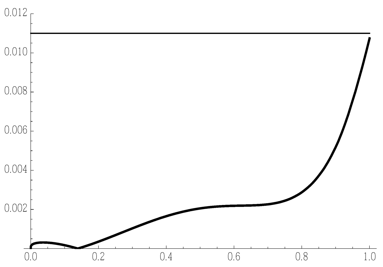
4. Notes on Absolute and Relative Errors

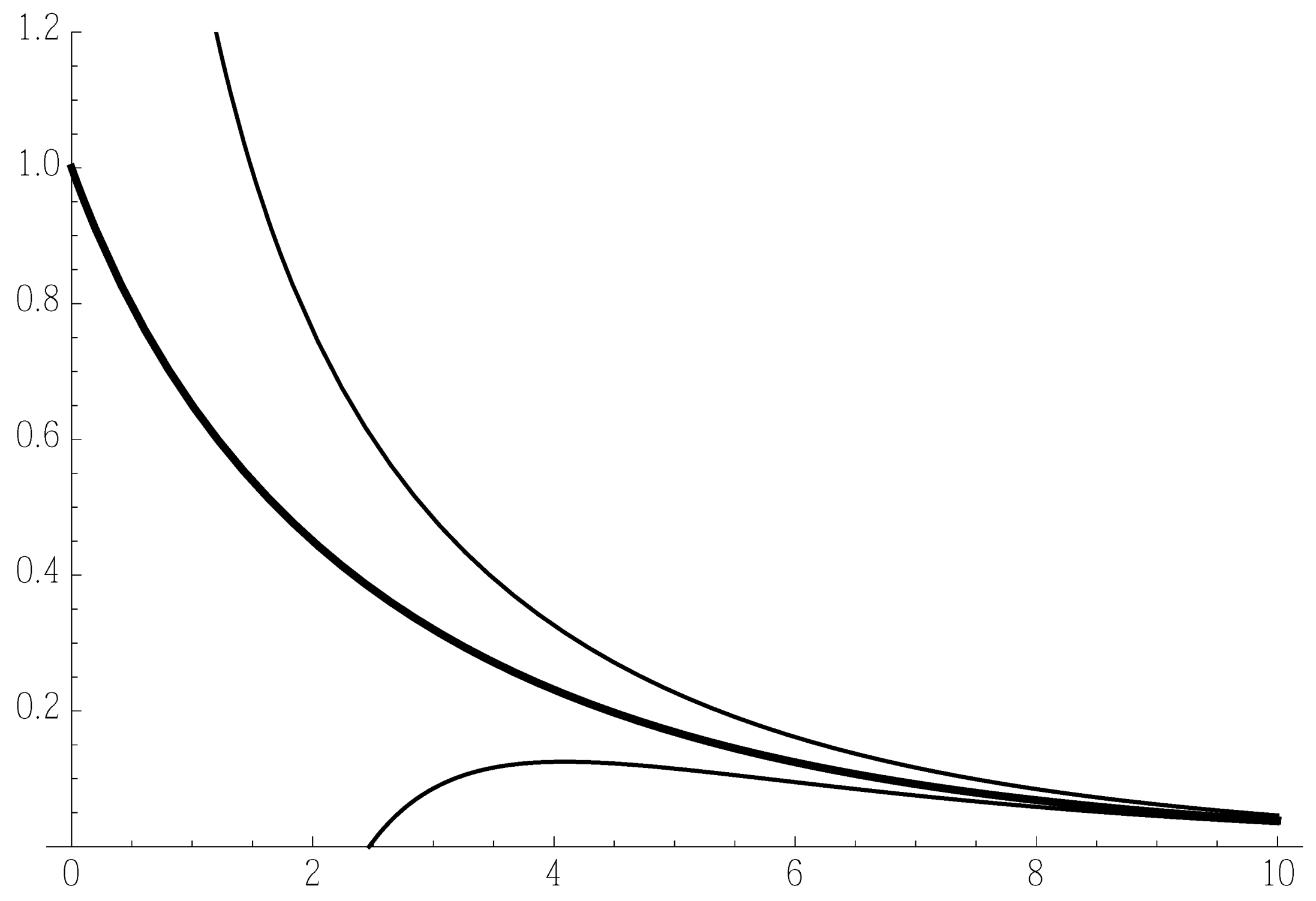
Let’s denote, for a function $f(·)$ and an approximation $a(·)$ of the same argument, by 

$${\epsilon }^{(f,a)}(·):=|a(·)-f(·)|,\mathrm{or}\mathrm{simply}{\epsilon }^{\left(f\right)}(·),\mathrm{or}\mathrm{even}\epsilon (·)$$

the absolute error, intended as a function with the same domain of f, and by

$${\epsilon }^{(f,a)}:=max|a(·)-f(·)|,\mathrm{or}\mathrm{simply}{\epsilon }^{(f,a)},\mathrm{or}\mathrm{even}\epsilon$$

the maximum absolute error, intended as a number, summarizing the distance of the approximation from the function.

Analogously, for relative errors, denote with

$${\epsilon }_r^{(f,a)}(·):=\left|\frac{a(·)-f(·)}{f(·)}\right|,\mathrm{or}\mathrm{simply}{\epsilon }_r(·)$$

(9)

the absolute relative error, intended as a function with the same domain of f if $\ne 0$, and by

$${\epsilon }_r^{(f,a)}:=max\left|\frac{a(·)-f(·)}{f(·)}\right|,\mathrm{or}\mathrm{simply}{\epsilon }_r$$

(10)

the maximum absolute relative error, intended as a number, summarizing the distance of the approximation from the function, normalized with respect to the function f itself, if $\ne 0$.

Generally, it may be observed that, when classifying two approximations of a function by means of their closeness to that function, the use of the relative error as a means of measuring this closeness is more suitable if that function has a zero limit (In fact, for example, it is not very important to notice that an approximated value of about, let us say, ${10}^{-5}$, has an absolute error less than, let us say, ${10}^{-4}$). Thus, for the fundamental function $\varphi \left(x\right)$ defined in (4), with a zero limit for $x\to \infty$ (see Figure 3 in [11], showing its graph), the use of relative errors is more significant and widely used in the literature: see [2,3,6,10], concerning the approximations for the fundamental function $\varphi \left(x\right)$, but also works concerning other functions having a zero limit, such as the already cited Gaussian probability integral $Q\left(x\right)$ (see [18,19,20,21,22] where the approximations for $Q\left(x\right)$ were all found, minimizing the absolute relative error). Here, the relative error has been evaluated by applying (9) and (10), and computing $\varphi \left(x\right)$ numerically through the following Mathematica^® statement [11]:

$$\mathtt{phi}[\mathtt{x}\_]:=\mathtt{1}-(\mathtt{1}/\mathtt{Sqrt}[\mathtt{4}\mathtt{Pi} \mathtt{x}\left]\right)\mathtt{NIntegrate}\left[\mathtt{Tanh}\right[\mathtt{u}/\mathtt{2}] \mathtt{Exp}[-(\mathtt{u}-\mathtt{x})\mathtt{^}\mathtt{2}/(\mathtt{4} \mathtt{x})],$$

{u,−200,200}, WorkingPrecision −>24]

The first line simply rewrites the first line of (4) to perform a numerical integration with the instruction NIntegrate. The second line specifies the integration interval and, through the instruction WorkingPrecision, how many digits of precision should be maintained in the computation. For the computations of this paper, the second line has been refined to

{u,−320,320}, WorkingPrecision −>40]

5. The Function $\varphi \left(x\right)$: Review of Its Principal Approximations

For the function $\varphi \left(x\right)$ defined in (4), these upper and lower bounds have been proved in [2]:

$$\left(1-\frac{3}{x}\right)\sqrt{\frac{\pi }{x}}{e}^{-x/4}<\varphi \left(x\right)<\left(1+\frac{1}{7x}\right)\sqrt{\frac{\pi }{x}}{e}^{-x/4}\mathrm{for}x\ne 0$$

(11)

and these others, tighter, have been proved recently in [3]:

$$\left(1-\frac{{\pi }^2}{4}\frac{1}{x}\right)\sqrt{\frac{\pi }{x}}{e}^{-x/4}<\varphi \left(x\right)<\sqrt{\frac{\pi }{x}}{e}^{-x/4}\mathrm{for}x\ne 0.$$

(12)

Moreover, the following three approximations, all piecewise defined, have been published in [2,3,6], respectively (The approximations, throughout the paper, have been named with a subscript reporting the name of the first author of the publication):

$$a_{\mathrm{Chung}}\left(x\right)=\left\{\begin{array}{cccc}{e}^{-0.4527x^{0.86}+0.0218}\hfill & \mathrm{if}\hfill & 0\le x\le 10\hfill & \left(\mathrm{a}\right)\hfill \\ \sqrt{\frac{\pi }{x}}{e}^{-x/4}\left(1-\frac{10}{7x}\right)\hfill & \mathrm{if}\hfill & x>10\hfill & \left(\mathrm{b}\right)\hfill \end{array}\right.$$

(13)

$$a_{\mathrm{Vatta}}\left(x\right)=\left\{\begin{array}{cccc}{e}^{-0.4527x^{0.864}+0.0218}\hfill & \mathrm{if}\hfill & 0\le x\le 10\hfill & \left(\mathrm{a}\right)\hfill \\ \sqrt{\frac{\pi }{x}}{e}^{-x/4}\left(1-\frac{{\pi }^2}{8x}\right)\hfill & \mathrm{if}\hfill & x>10\hfill & \left(\mathrm{b}\right)\hfill \end{array}\right.$$

(14)

$$a_{\mathrm{Ha}}\left(x\right)=\left\{\begin{array}{cccc}{e}^{0.0564x^2-0.48560x}\hfill & \mathrm{if}\hfill & 0\le x<0.867861\hfill & \left(\mathrm{a}\right)\hfill \\ e^{-0.4527x^{0.86}+0.0218}\hfill & \mathrm{if}\hfill & 0.867861\le x\le 10\hfill & \left(\mathrm{b}\right)\hfill \\ \sqrt{\frac{\pi }{x}}{e}^{-x/4}\left(1-\frac{10}{7x}\right)\hfill & \mathrm{if}\hfill & x>10\hfill & \left(\mathrm{c}\right).\hfill \end{array}\right.$$

(15)

As remarked in [10], (8) can be solved making use of an explicitly invertible approximation of $\varphi \left(x\right)$, since $g_s\left(t\right)$ is defined through $\varphi$ and ${\varphi }^{-1}$.

The piecewise defined approximation found in [2], and recalled in (13), is made of two parts: the first, holding for $0\le x\le 10$, is the ad hoc approximation by elementary functions (13a), explicitly invertible, the second, holding for $x>10$, is the approximation (13b), instead not explicitly invertible, and therefore, not usable directly in (8). Thus, to solve (8), in [15] Babich et al. have used the approximation (13a) only, which behaves very badly, as shown in Figure 1 of [10], for $x>10$. In this case, the more the argument of $\varphi \left(x\right)$ gets greater than 10 in the sequence defined by (7), the more uncertain are the GA thresholds evaluated solving (8), with respect to the exact ones ${\sigma }_{\mathrm{exact}}$ evaluated through density evolution, e.g., in [12].

The piecewise defined approximation found in [3], and recalled in (14), also contains, for $0\le x\le 10$, an explicitly invertible ad hoc approximation (14a), obtained through elementary functions [10]. The approximation (14b) of [3] for $x>10$, is instead not explicitly invertible again, like the one in [2], and thus again not usable directly in (8) to find its solution. Thus, to find the numerical results published in [2,3], their authors had to resort (even not explicitly stated in [2,3]) to an interpolated function approximating (13b) and (14b) by points to determine its inverse, needed to solve (8) (since it is defined through (5) and (6)).

To avoid the abovementioned problems, a new, explicitly invertible, approximation of $\varphi \left(x\right)$ was given in [10]. This was not defined by multiple functions, but by a unique expression (the subscript “np” stands for “not piecewise” (defined)):

$$a_{\mathrm{Vatta}-\mathrm{np}}\left(x\right)=\psi \left(\nu \left(\mu \left(x\right)\right)\right)\approx \varphi \left(x\right)$$

(16)

being

$$\psi \left(z\right):=\sqrt{\frac{\pi }{z}}{e}^{-z/4}$$

$$z=\nu \left(y\right):=y+\frac{a}{b+y}y=\mu \left(x\right):=x+c{e}^{dx}$$

with

$$a=(b+c)\left(2W\left(\frac{\pi }{2}\right)-c\right)b=6.45$$

$$c=-0.062d=-1.87,$$

where $W\left(x\right)$ is the Lambert $W$-function, and $a_{\mathrm{Vatta}-\mathrm{np}}\left(x\right)$ is the new approximation of $\varphi \left(x\right)$, defined by a single expression for any $x\ge 0$. To build an approximation $a\left(x\right)$ of $\varphi \left(x\right)$, having the two fundamental characteristics mentioned at the end of Section 3, the function

$$\psi \left(z\right):=\sqrt{\frac{\pi }{z}}{e}^{-z/4}$$

was taken as a fundamental function, since, as remarked in the Appendix of [5], it is a good explicitly invertible asymptotical approximation of $\varphi \left(x\right)$, but-as observed in [10]—it diverges in $x=0$, giving an infinite maximum absolute relative error ${\epsilon }_r$ (see Table 1 in [10]), and its inverse presents an infinite maximum absolute relative error ${\epsilon }_r$, too, since ${\psi }^{-1}\left(1\right)\approx 1.5$ (i.e., $\ne 0$).

In [10], some suitable functions $\nu \left(y\right)$, $\mu \left(x\right)$, and parameters a, b, c, and d have been explored to detect the most appropriate approximation. The fitting parameter a was selected so that $a_{\mathrm{Vatta}-\mathrm{np}}\left(0\right)=1$ precisely and, therefore, $a_{\mathrm{Vatta}-\mathrm{np}}^{-1}\left(1\right)=0$ (see the function ${\psi }^{-1}\left(y\right)$ derived in the Appendix of [5]), thus fulfilling the two fundamental points mentioned at the end of Section 3. The functions $\nu \left(y\right)$, $\mu \left(x\right)$, and the parameters b, c, and d have been searched with the goal of minimizing the absolute relative error (9), while maintaining the explicit invertibility.

In Figure 2 of [10], it was shown that the relative error of $a_{\mathrm{Vatta}-\mathrm{np}}\left(x\right)$ is <0.14% in $[0,80]$, which is the interval of main interest, where the approximation (16) remains between the two tighter bounds (12) defined in [3] as shown in Figure 1. Furthermore, as shown in

Table 1. Maximum absolute relative errors ${\epsilon }_r$ (10) of the different approximations of the function $\varphi \left(x\right)$ and of its inverse, when it exists.

Eq.	First Author (Year) [Ref.]	Parts	Domain	${\mathit{\epsilon }}_{\mathit{r}}$	${\mathit{\epsilon }}_{\mathit{r}}$ for the Inverse
(13a)	Chung (2001) [2]	1	$0\le x\le 10$	$2.3\%$	$+\infty$
(14a)	Vatta (2019) [3]	1	$0\le x\le 10$	$3.0\%$	$+\infty$
(15a)	Ha (2004) [6]	1	$0\le x<0.867861$	$0.1\%$	$3\%$
(13b)	Chung (2001) [2]	1	$x>10$	$3.1\%$	$0.9\%$
(14b)	Vatta (2019) [3]	1	$x>10$	$4.9\%$	$1.7\%$
(13)	Chung (2001) [2]	2	$x>0$	$3.1\%$	$\nexists$
(14)	Vatta (2019) [3]	2	$x>0$	$4.9\%$	$\nexists$
(15)	Ha (2004) [6]	3	$x\ge 0$	$3.1\%$	$\nexists$
(16)	Vatta (2019)	1	$x\ge 0$	0.14%	1.1%

, it has a lower maximum absolute relative error ${\epsilon }_r$ (10)—reported in bold—than any other approximation, except (15a) (In [6], the authors had to add the ad hoc explicitly invertible approximation (15a), since they had to compute $\varphi \left(x\right)$ around $x=0$, where the approximation (13a) is not good enough (see Figure 1 of [10])).

6. Approximating the Function ${\varphi }^{-1}\left(y\right)$ through an Explicitly Invertible Approximation

The explicit invertibility of an approximation $a\left(x\right)$ avoids the necessity of making use of an interpolated function to approximate it by points $(x_k,a\left(x_k\right))$ and its inverse by points $(a\left(x_k\right),x_k)$ [10]. In other words, we assume that a function is explicitly invertible if we are able to find an inverse whose expression involves elementary functions and the Lambert $W$-function. Here, this property will be explained through an example, showing how to find an inverse with these characteristics.

6.1. Example of Explicit Invertibility

Given the function

$$y\left(x\right):=\frac{a{\mathrm{e}}^{-b{(x+d)}^c}}{{({(x+d)}^c+s)}^t},$$

the procedure to obtain the explicit inverse goes through the following steps:

• substitute $u:=x+d$ or $x=u-d$ thus obtaining

  $$y=\frac{a{\mathrm{e}}^{-b{u}^c}}{{(u^c+s)}^t};$$
• substitute $w:=u^c$ or $u=w^{1/c}$ getting

  $$y=\frac{a{\mathrm{e}}^{-bw}}{{(w+s)}^t};$$
• substitute $z:=w+s$ or $w=z-s$ thus giving

  $$y=\frac{a{\mathrm{e}}^{-b(z-s)}}{z^t};$$
• expand

  $$y=\frac{a{\mathrm{e}}^{-bz+bs}}{z^t}=\left(a{\mathrm{e}}^{bs}\right)\frac{{\mathrm{e}}^{-bz}}{z^t};$$
• define the constant $k:=a{\mathrm{e}}^{bs}$ obtaining

  $$y=k\frac{{\mathrm{e}}^{-bz}}{z^t};$$
• and rewrite the last, yielding the following:

  $$\frac{b}{t}{\left(\frac{y}{k}\right)}^{-1/t}=\frac{bz}{t}{\mathrm{e}}^{\frac{bz}{t}}.$$
• Finally, recalling that $W\left(x{e}^x\right)\equiv x$ for $x>0$ (see, e.g., [5]) invert the last obtaining this function (of the variable y)

  $$z=\frac{t}{b}W\left(\frac{b{\left(\frac{y}{k}\right)}^{-1/t}}{t}\right),$$
• and then make the aforementioned substitutions:

  $$k=a{\mathrm{e}}^{bs}\Rightarrow z=\frac{t}{b}W\left(\frac{b{\left(\frac{y}{a{\mathrm{e}}^{bs}}\right)}^{-1/t}}{t}\right)$$

  $$z=w+s\Rightarrow w+s=\frac{t}{b}W\left(\frac{b{\left(\frac{y}{a{\mathrm{e}}^{bs}}\right)}^{-1/t}}{t}\right)$$

  $$w=u^c\Rightarrow u^c+s=\frac{t}{b}W\left(\frac{b{\left(\frac{y}{a{\mathrm{e}}^{bs}}\right)}^{-1/t}}{t}\right)$$

  $$u=x+d\Rightarrow {(x+d)}^c+s=\frac{t}{b}W\left(\frac{b{\left(\frac{y}{a{\mathrm{e}}^{bs}}\right)}^{-1/t}}{t}\right)$$
• yielding

  $${(x+d)}^c=\frac{t}{b}W\left(\frac{b{\left(\frac{y}{a{\mathrm{e}}^{bs}}\right)}^{-1/t}}{t}\right)-s$$

  and

  $$(x+d)={\left(\frac{t}{b}W\left(\frac{b{\left(\frac{y}{a{\mathrm{e}}^{bs}}\right)}^{-1/t}}{t}\right)-s\right)}^{1/c}$$
• Thus, the explicit inverse of the starting function $y\left(x\right)$ can be expressed as

  $$x={\left(\frac{t}{b}W\left(\frac{b{\left(\frac{y}{a{\mathrm{e}}^{bs}}\right)}^{-1/t}}{t}\right)-s\right)}^{1/c}-d$$

6.2. Explicit Inverse of the Approximation $a_{\mathrm{Vatta}-\mathrm{np}}\left(x\right)$

Since the approximation $a_{\mathrm{Vatta}-\mathrm{np}}\left(x\right)$ (16) is made of the three explicitly invertible functions $\psi$, $\nu$ and $\mu$, it is explicitly invertible by the Lambert $W$-function [10]:

$$\psi \left(\nu \right(\mu \left(x\right)\left)\right)=y$$

$$\nu \left(\mu \left(x\right)\right)={\psi }^{-1}\left(y\right)\mu \left(x\right)={\nu }^{-1}\left({\psi }^{-1}\left(y\right)\right)$$

$$x={\mu }^{-1}\left({\nu }^{-1}\left({\psi }^{-1}\left(y\right)\right)\right)=a_{\mathrm{Vatta}-\mathrm{np}}^{-1}\left(y\right)\approx {\varphi }^{-1}\left(y\right)$$

with

$${\psi }^{-1}\left(y\right)=2W\left(\frac{\pi }{2y^2}\right)$$

$${\nu }^{-1}\left(y\right)=\frac{1}{2}\left(\sqrt{-4a+b^2+2by+y^2}-b+y\right)$$

$${\mu }^{-1}\left(y\right)=\frac{dy-W\left(cd{e}^{dy}\right)}{d}.$$

The inverse $a_{\mathrm{Vatta}-\mathrm{np}}^{-1}\left(y\right)$ of the approximation $a_{\mathrm{Vatta}-\mathrm{np}}\left(x\right)$, considered as an approximation of the inverse ${\varphi }^{-1}\left(y\right)$ of $\varphi \left(x\right)$, has a maximum absolute relative error ${\epsilon }_r$ (10) of $1.1\%$ in its domain $\left[\psi \right(80),1]$, which is the interval of main interest, being $\psi \left(80\right)\approx 0$, as shown in Figure 2. This is less than the maximum absolute relative error of any other approximation inverse, when it exists, except (13b) (In [2], for $x>10$ the authors suggest to use the approximation (13b), average of the upper and lower bound (11) which, like (14b), the average of the upper and lower bound (12), is not explicitly invertible), as shown in Table 1 (in bold).

As mentioned at the end of Section 3, the approximation of the inverse in $y=1$ must match ${\varphi }^{-1}\left(1\right)$ exactly, otherwise it gives rise to an infinite maximum absolute relative error for the inverse (last column of Table 1) in 1, since ${\varphi }^{-1}\left(1\right)=0$. This happens to the approximation (13a), for which $a_{\mathrm{Chung}}^{-1}\left(1\right)\approx {\left(\frac{0.0218}{0.4527}\right)}^{1/0.86}\ne 0$ (see [15], where the inverse of (13a) has been derived in (6)), and to the approximation (14a), whose inverse may be expressed as follows:

$$a_{\mathrm{Vatta}}^{-1}\left(y\right)={\left(\frac{logy-\beta }{\alpha }\right)}^{1/\gamma },$$

(17)

with $\alpha =-0.4527$, $\beta =0.0218$, and $\gamma =0.864$. In this case, $a_{\mathrm{Vatta}}^{-1}\left(1\right)\approx {\left(\frac{0.0218}{0.4527}\right)}^{1/0.864}\ne 0$ yields an infinite maximum absolute relative error for the inverse.

7. Numeric Results Concerning the Computation of the GA Thresholds and Discussion

Generalizing Luby et al.’s results reported in [23], Richardson and Urbanke have proved a concentration principle in [24]. In particular, they have shown that the average behaviour of the individual instances of a code tends to concentrate around its expected behaviour, obtained when its length is supposed to grow. In other words, they showed that this average behaviour converges to the behaviour of the cycle-free case, which can be derived from the corresponding cycle-free Tanner graph. They defined the threshold, as explained in the Introduction, for a random ensemble of irregular LDPC codes, specified by their degree distributions (1) and (2). Moreover, they presented an algorithm, denoted as the density evolution algorithm, for the determination of the thresholds through iteratively calculated message densities.

In this section, we present a comparison (see

Table 2. GA thresholds calculated by applying different approximations of the function $\varphi \left(x\right)$ and of its inverse.

Eq.	First Author (Year) [Ref.]	Domain	GA Threshold
(13)	Chung (2001) [2]	$x>0$	${\sigma }_{\mathrm{GA}\mathrm{Chung}}=0.9473$
			${\sigma }_{\mathrm{GA}0.05}=0.9519$
(14)	Vatta (2019) [3]	$x>0$	${\sigma }_{\mathrm{GA}0.1}=0.9538$
			${\sigma }_{\mathrm{GA}0.5}=0.9533$
(16)	Vatta (2019) [10]	$x\ge 0$	${\sigma }_{\mathrm{GA}\mathrm{Vatta}-\mathrm{np}}=0.9526$

) between the GA thresholds, calculated by applying the procedure described throughout this paper, and the thresholds calculated through the density evolution algorithm. These thresholds have been shown in [24] to be approached more closely as the codeword lengths increase (see Figures 5 and 6 in [24], where the bit error rate performance curves are shown to move closer to the density evolution thresholds, denoted by ${\sigma }^{\ast }$, as the block lengths increase from 1000 to 100,000). This corresponds to making a comparison between the GA thresholds and those obtained by applying a message passing algorithm to the iterative decoding of a long deterministic LDPC code.

For the irregular rate-1/2 LDPC code given in [2], with $d_l=20$ and $d_r=9$, with degree distributions

$$\begin{array}{cc}\lambda \left(x\right)=\hfill & 0.23403x+0.21242x^2+0.14690x^5+0.10284x^6\hfill \\ \hfill & +0.30381x^{19}\hfill \\ \rho \left(x\right)=\hfill & 0.71875x^7+0.28125x^8\hfill \end{array}$$

(18)

in [3], applying the software of [15] and the piecewise defined approximation (14), a GA threshold was calculated ${\sigma }_{\mathrm{GA}\mathrm{Vatta}}=0.9538$, which was closer to the density evolution one ${\sigma }_{\mathrm{exact}}=0.9669$ (reported in [2]) than the GA threshold ${\sigma }_{\mathrm{GA}\mathrm{Chung}}=0.9473$ computed in [2] using the piecewise defined approximation (13). As said in Section 5, to find the numerical results published in [2,3], their authors had to resort (even not explicitly stated) to an interpolated function approximating (13b) and (14b) by points $(x_k,a\left(x_k\right))$ to determine its inverse by points $(a\left(x_k\right),x_k)$, needed to solve (8). As far as the function interpolation (14b) is concerned, we found that the GA threshold computed through it depends on the interpolation step $\Delta x$ considered. Taking, e.g., an interpolation step $\Delta x=0.5$, we computed a GA threshold ${\sigma }_{\mathrm{GA}0.5}=0.9533$, with $\Delta x=0.1$ a GA threshold ${\sigma }_{\mathrm{GA}0.1}=0.9538$ (the one reported in [3]), and with $\Delta x=0.05$, a GA threshold ${\sigma }_{\mathrm{GA}0.05}=0.9519$. By instead applying the new, not piecewise defined, approximation (16), we obtain ${\sigma }_{\mathrm{GA}\mathrm{Vatta}-\mathrm{np}}=0.9526$, which is closer to the density evolution threshold ${\sigma }_{\mathrm{exact}}=0.9669$ than ${\sigma }_{\mathrm{GA}0.05}=0.9519$ and ${\sigma }_{\mathrm{GA}\mathrm{Chung}}=0.9473$, but is slightly looser than ${\sigma }_{\mathrm{GA}0.5}=0.9533$ and ${\sigma }_{\mathrm{GA}0.1}=0.9538$. However, using (16), the solution of (8) is greatly simplified since, as noticed in [10], this approximation is given in $[0,+\infty [$ by a single expression. This implies that, in any argument x, it presents a unique analytical expression permitting its straightforward algebraic manipulation. On the other hand, the so-called piecewise defined functions present different analytical expressions determined by the value taken by the argument x. Moreover, by using it, the solution of (8) does not depend on any discretization step.

8. Conclusions

In this paper, a review of old and new approximations to the function $\varphi \left(x\right)$, characterizing the passage of messages between variable and check nodes of the bipartite graph describing an LDPC code [1], has been performed. In particular, two old (published in 2001 and 2004, respectively) and two new approximations, recently published, to the function $\varphi \left(x\right)$, were reviewed to analyze the differences among them and their characteristics in terms of accuracy and computational complexity. The second of the two new approximations, unlike the other three (two old and one new) is defined by a single expression (i.e., it is not piecewise defined), it is explicitly invertible by means of the Lambert $W$-function, it remains between the two tighter bounds (12) recently defined in [3], and it has a lower relative error in any x than most of the other approximations (With the only exception of the explicitly invertible approximation (15a), valid only for $0\le x<0.867861$) when the error is evaluated using a numerical computation of $\varphi \left(x\right)$. As remarked in [10], the fact that it is defined by a single expression and it is explicitly invertible yield an important complexity reduction of the algebraic handling of the approximation itself. Moreover, its use allows better GA thresholds to be obtained, in the sense that they approximate the thresholds obtained with density evolution better than the GA thresholds obtained in [2].

References

1. Tanner, R.M. A recursive approach to low complexity codes. IEEE Trans. Inf. Theory 1981, 27, 533–547. [Google Scholar] [CrossRef] [Green Version]
2. Chung, S.-Y.; Richardson, T.J.; Urbanke, R. Analysis of sum-product decoding of low-density parity-check codes using a Gaussian approximation. IEEE Trans. Inf. Theory 2001, 47, 657–670. [Google Scholar] [CrossRef] [Green Version]
3. Vatta, F.; Soranzo, A.; Babich, F. More accurate analysis of sum-product decoding of LDPC codes using a Gaussian approximation. IEEE Commun. Lett. 2019, 23, 230–233. [Google Scholar] [CrossRef] [Green Version]
4. Vatta, F.; Soranzo, A.; Comisso, M.; Buttazzoni, G.; Babich, F. Performance study of a class of irregular LDPC codes through low complexity bounds on their belief-propagation decoding thresholds. In Proceedings of the 2019 AEIT International Annual Conference, AEIT 2019, Florence, Italy, 18–20 September 2019. [Google Scholar]
5. Vatta, F.; Soranzo, A.; Babich, F. Low-Complexity bound on irregular LDPC belief-propagation decoding thresholds using a Gaussian approximation. Electron. Lett. 2018, 54, 1038–1040. [Google Scholar] [CrossRef] [Green Version]
6. Ha, J.; Kim, J.; McLaughlin, S.W. Rate-compatible puncturing of low-density parity-check codes. IEEE Trans. Inf. Theory 2004, 50, 2824–2836. [Google Scholar] [CrossRef]
7. Babich, F.; Noschese, M.; Soranzo, A.; Vatta, F. Low complexity rate compatible puncturing patterns design for LDPC codes. J. Commun. Softw. Syst. (JCOMSS) 2018, 14, 350–358. [Google Scholar] [CrossRef]
8. Tan, B.S.; Li, K.H.; Teh, K.C. Bit-error rate analysis of low-density parity- check codes with generalised selection combining over a Rayleigh-fading channel using Gaussian approximation. IET Commun. 2012, 6, 90–96. [Google Scholar] [CrossRef]
9. Chen, X.; Lau, F.C.M. Optimization of LDPC codes with deterministic unequal error protection properties. IET Commun. 2011, 5, 1560–1565. [Google Scholar] [CrossRef]
10. Vatta, F.; Soranzo, A.; Comisso, M.; Buttazzoni, G.; Babich, F. New explicitly invertible approximation of the function involved in LDPC codes density evolution analysis using a Gaussian approximation. Electron. Lett. 2019, 55, 1183–1186. [Google Scholar] [CrossRef]
11. Babich, F.; Noschese, M.; Soranzo, A.; Vatta, F. Low complexity rate compatible puncturing patterns design for LDPC codes. In Proceedings of the 2017 International Conference on Software, Telecommunications and Computer Networks, SoftCOM’17, Split, Croatia, 21–23 September 2017. [Google Scholar]
12. Richardson, T.J.; Shokrollahi, A.; Urbanke, R. Design of capacity-approaching irregular low-density parity-check codes. IEEE Trans. Inf. Theory 2001, 47, 619–637. [Google Scholar] [CrossRef] [Green Version]
13. Vatta, F.; Babich, F.; Ellero, F.; Noschese, M.; Buttazzoni, G.; Comisso, M. Role of the product λ(0)ρ(1) in determining LDPC code performance. Electronics 2019, 8, 1515. [Google Scholar] [CrossRef] [Green Version]
14. Vatta, F.; Babich, F.; Ellero, F.; Noschese, M.; Buttazzoni, G.; Comisso, M. Performance study of a class of irregular LDPC codes based on their weight distribution analysis. In Proceedings of the 2019 International Conference on Software, Telecommunications and Computer Networks, SoftCOM’19, Split, Croatia, 19–21 September 2019. [Google Scholar]
15. Babich, F.; Soranzo, A.; Vatta, F. Useful mathematical tools for capacity approaching codes design. IEEE Commun. Lett. 2017, 21, 1949–1952. [Google Scholar] [CrossRef]
16. Hale, J.; Koçak, H. Dynamics and Bifurcations; Springer: Berlin, Germany, 1991. [Google Scholar]
17. Olabiyi, O.; Annamalai, A. Invertible exponential-type approximations for the Gaussian probability integral Q(x) with applications. IEEE Wirel. Commun. Lett. 2012, 1, 544–547. [Google Scholar] [CrossRef]
18. Borjesson, P.O.; Sundberg, C.-E.W. Simple approximations of the error function Q(x) for communications applications. IEEE Trans. Commun. 1979, 27, 639–643. [Google Scholar] [CrossRef]
19. Chiani, M.; Dardari, D.; Simon, M.K. New exponential bounds and approximations for the computation of error probability in fading channels. IEEE Trans. Wirel. Commun. 2003, 2, 840–845. [Google Scholar] [CrossRef] [Green Version]
20. Shi, Q.; Karasawa, Y. An accurate and efficient approximation to the Gaussian Q-function and its applications in performance analysis in Nakagami-m fading. IEEE Commun. Lett. 2011, 15, 479–481. [Google Scholar]
21. Benitez, M.; Casadevall, F. Versatile, accurate, and analytically tractable approximation for the Gaussian Q-function. IEEE Trans. Commun. 2011, 59, 917–922. [Google Scholar] [CrossRef] [Green Version]
22. Soranzo, A.; Vatta, F.; Comisso, M.; Buttazzoni, G.; Babich, F. New very simply explicitly invertible approximation of the Gaussian Q-function. In Proceedings of the 2019 International Conference on Software, Telecommunications and Computer Networks, SoftCOM’19, Split, Croatia, 19–21 September 2019. [Google Scholar]
23. Luby, M.G.; Mitzenmacher, M.; Shokrollahi, M.A.; Spielman, D.A. Improved low-density parity-check codes using irregular graphs. IEEE Trans. Inf. Theory 2001, 47, 585–598. [Google Scholar] [CrossRef] [Green Version]
24. Richardson, T.J.; Urbanke, R. The capacity of low-density parity-check codes under message-passing decoding. IEEE Trans. Inf. Theory 2001, 47, 599–618. [Google Scholar] [CrossRef]
Figure 1. Graphs in [ 0 , 10 ] of the function a Vatta np ( x ) (approximating ϕ ( x ) ) (16) (bold) and the tighter lower and upper bounds (12).
Information 12 00212 g001
Figure 2. Relative error (in absolute value) ε r ( y ) (9) of a Vatta np 1 ( y ) .
Information 12 00212 g002