
Distributed Hypothesis Testing over Noisy Broadcast Channels

1
Department of Electrical and Computer Engineering, College of Engineering, University of Tehran, Tehran 1433957131, Iran
2
LTCI, Telecom Paris, IP Paris, 91120 Paris, France
*
Author to whom correspondence should be addressed.
†
M. Wigger has received funding from the European Research Council (ERC) under the European Union’s Horizon 2020 programme, grant agreement No 715111.
Information 2021, 12(7), 268; https://0-doi-org.brum.beds.ac.uk/10.3390/info12070268
Submission received: 21 May 2021
/
Revised: 8 June 2021
/
Accepted: 8 June 2021
/
Published: 29 June 2021
(This article belongs to the Special Issue Statistical Communication and Information Theory)
Abstract
:This paper studies binary hypothesis testing with a single sensor that communicates with two decision centers over a memoryless broadcast channel. The main focus lies on the tradeoff between the two type-II error exponents achievable at the two decision centers. In our proposed scheme, we can partially mitigate this tradeoff when the transmitter has a probability larger than to distinguish the alternate hypotheses at the decision centers, i.e., the hypotheses under which the decision centers wish to maximize their error exponents. In the cases where these hypotheses cannot be distinguished at the transmitter (because both decision centers have the same alternative hypothesis or because the transmitter’s observations have the same marginal distribution under both hypotheses), our scheme shows an important tradeoff between the two exponents. The results in this paper thus reinforce the previous conclusions drawn for a setup where communication is over a common noiseless link. Compared to such a noiseless scenario, here, however, we observe that even when the transmitter can distinguish the two hypotheses, a small exponent tradeoff can persist, simply because the noise in the channel prevents the transmitter to perfectly describe its guess of the hypothesis to the two decision centers.
1. Introduction
In Internet of Things (IoT) networks, data are collected at sensors and transmitted over a wireless channel to remote decision centers, which decide on one or multiple hypotheses based on the collected information. In this paper, we study simple binary hypothesis testing with a single sensor but two decision centers. The results can be combined with previous studies focusing on multiple sensors and a single decision center to tackle the practically relevant case of multiple sensors and multiple decision centers. We consider a single sensor for simplicity and because our main focus is on studying the tradeoff between the performances at the two decision centers that can arise because the single sensor has to send information over the channel that can be used by both decision centers. A simple, but highly suboptimal, approach would be to time-share communication and serve each of the two decision centers only during a part of the transmission. As we will see, better schemes are possible, and, in some cases, it is even possible to serve each of the two decision centers as if the other center was not present in the system.
In this paper, we follow the information-theoretic framework introduced in [1,2]. That means each terminal observes a memoryless sequence, and depending on the underlying hypothesis , all sequences follow one of two possible joint distributions, which are known to all involved terminals. A priori, the transmitter, however, ignores the correct hypothesis and has to compute its transmit signal as a function of the observed source symbols only. Decision centers observe outputs of the channel, and, combined with their local observations, they have to make a decision on whether or . The performance of the decision center is measured by its type-II error exponent, i.e., the expontial decay in the length of the observations of the probability of deciding on when the true hypothesis is . As a constraint on the decision center, we impose that the type-I error probability, i.e., the probability of deciding when the true hypothesis is , vanishes (at any desired speed) with increasing observation lengths. The motivation for studying such asymmetric requirements on the two error probabilities stems, for example, from alert systems, where the miss-detection event is much more harmful than the false-alarm event, and, as a consequence, in our systems we require the miss-detection probability to decay much faster than the false-alarm probability.
This problem setting has first been considered for the setup with a single sensor and a single decision center when communication is over a noiseless link of given capacity [1,2]. For this canonical problem, the optimal error exponent has been identified in the special cases of testing against independence [1] and testing against conditional independence [3,4].
The scheme proposed by Shimokawa–Han–Amari in [3,4] yields an achievable error exponent for all distributed hypothesis testing problems (not only testing against conditional independence) [3,4], but it might not be optimal in general [5]. The Shimokawa–Han–Amari (SHA) scheme has been extended to various more involved setups such as noiseless networks with multiple sensors and a single decision center [2,6,7]; networks where the sensor and the decision center can communicate interactively [8,9]; multi-hop networks [10]; networks with multiple decision centers [10,11,12,13].
The works most closely related to the current paper are [10,12,13,14,15,16]. Specifically, Refs [10,12,13,14] consider a single-sensor multi-detector system where communication is over a common noiseless link from the sensor to all decision centers. Focusing on two decision centers, two scenarios can be encountered here: (1) the two decision centers have the same null and alternate hypotheses, and as a consequence, both aim at maximizing the error exponent under the same hypothesis ; or (2) the two decision centers have opposite null and alternate hypotheses and thus one decision center wishes to maximize the error exponent under hypothesis and the other under hypothesis . The second scenario is motivated by applications where the decision centers have different goals. Hypothesis testing for scenario 1) was studied in [10,12,13,14], and the results showed a tradeoff between the exponents achieved at the two decision centers. Intuitively, the tradeoff comes from the fact that communication from the sensor is serving both decision centers at the same time. Scenario 2) was considered in [12,13]. In this case, a tradeoff only occurs when the sensor’s observation alone provides no advantage in guessing the hypothesis. Otherwise, a tradeoff-free exponent region can be achieved by the following simple scheme: the sensor takes a tentative guess on the hypothesis based only on its local observations. It communicates this tentative guess to both decision centers using a single bit and then dedicates the rest of the communication using a dedicated SHA scheme only to the decision center that wishes to maximize the error exponent under the hypothesis that does not correspond to its guess. The other decision center simply keeps the transmitter’s tentative guess and ignores the rest of the communication.
In this paper, we extend these previous works to memoryless broadcast channels (BC). Hypothesis testing over BCs was already considered in [10], however, only for above scenario 1 where both decision centers have the same null and alternate hypothesis and in the special case of testing against conditional independence, in which case the derived error exponents were proved to be optimal. Interestingly, when testing against conditional independence over noisy channels, only the capacity of the channel matters but not the properties, see [15,16]. General hypothesis testing over noisy channels is much more challenging and requires additional tools, such as joint source-channel coding and unequal error protection (UEP) coding [17]. The latter can, in particular, be used to specially protect the communication of the sensor’s tentative guess, which allows one to avoid a degradation of the performance of classical hypothesis testing schemes.
We present general distributed hypothesis testing schemes over memoryless BCs, and we analyze the performances of these schemes with a special focus on the tradeoff in exponents they achieve for the two decision centers. We propose two different schemes, depending on whether the sensor can distinguish with error probability the two null hypotheses at the two decision centers. If a distinction is possible (because the decision centers have different null hypothesis and the sensor’s observations follow different marginal distributions under the two hypotheses), then we employ a similar scheme as proposed in [12,13] over a common noiseless link, but where the SHA scheme is replaced by the UEP-based scheme for DMCs in [15]. That means, the sensor makes a tentative guess about the hypothesis and conveys this guess to both decision centers using an UEP mechanism. Moreover, the joint source-channel coding scheme in [15] with dedicated codebooks is used to communicate to the decision center that aims to maximize the error exponent under the hypothesis that does not correspond to the sensor’s tentative guess. This scheme shows no tradeoff between the exponents achieved at the two decision centers in various interesting cases. Sometimes, however, a tradeoff arises because even under UEP the specially protected messages can be in error and because the decision centers can confuse the codewords of the two different sets of codebooks. For the case where the sensor cannot reasonably distinguish the alternate hypotheses at the two decision centers (because both decision centers have the same alternate hypotheses or the sensor’s observations have the same marginal observations under both hypotheses), we present a scheme similar to [10] but again including UEP. In this scheme, a tradeoff between the exponents achieved at the two decision centers naturally arises and mostly stems from the inherent tradeoff in distributed lossy compression systems with multiple decoders having different side informations.
Notation
We mostly follow the notation in [18]. Random variables are denoted by capital letters, e.g., , , and their realizations by lower-case letters, e.g., , y. Script symbols such as and stand for alphabets of random variables, and and for the corresponding n-fold Cartesian products. Sequences of random variables and realizations are abbreviated by and . When , then we also use and instead of and .
We write the probability mass function (pmf) of a discrete random variable X as ; to indicate the pmf under hypothesis , we also use . The conditional pmf of X given Y is written as , or as when . The term stands for the Kullback–Leibler (KL) divergence between two pmfs P and Q over the same alphabet. We use to denote the joint type of the pair of sequences , and cond_tp for the conditional type of given . For a joint type over alphabet , we denote by the conditional ßmutual information assuming that the random triple has pmf ; similarly for the entropy and the conditional entropy . Sometimes we abbreviate by . In addition, when has been defined and is clear from the context, we write or for the corresponding subtypes. When the type coincides with the actual pmf of a triple , we omit the subscript and simply write , , and .
For a given and a constant , let be the set of μ-typical sequences in as defined in [8] (Section 2.4). Similarly, stands for the set of jointly μ-typical sequences. The expectation operator is written as . We abbreviate independent and identically distributed by i.i.d. The log function is taken with base 2. Finally, in our justifications, we use (DP) and (CR) for “data processing inequality” and “chain rule”.
2. System Model
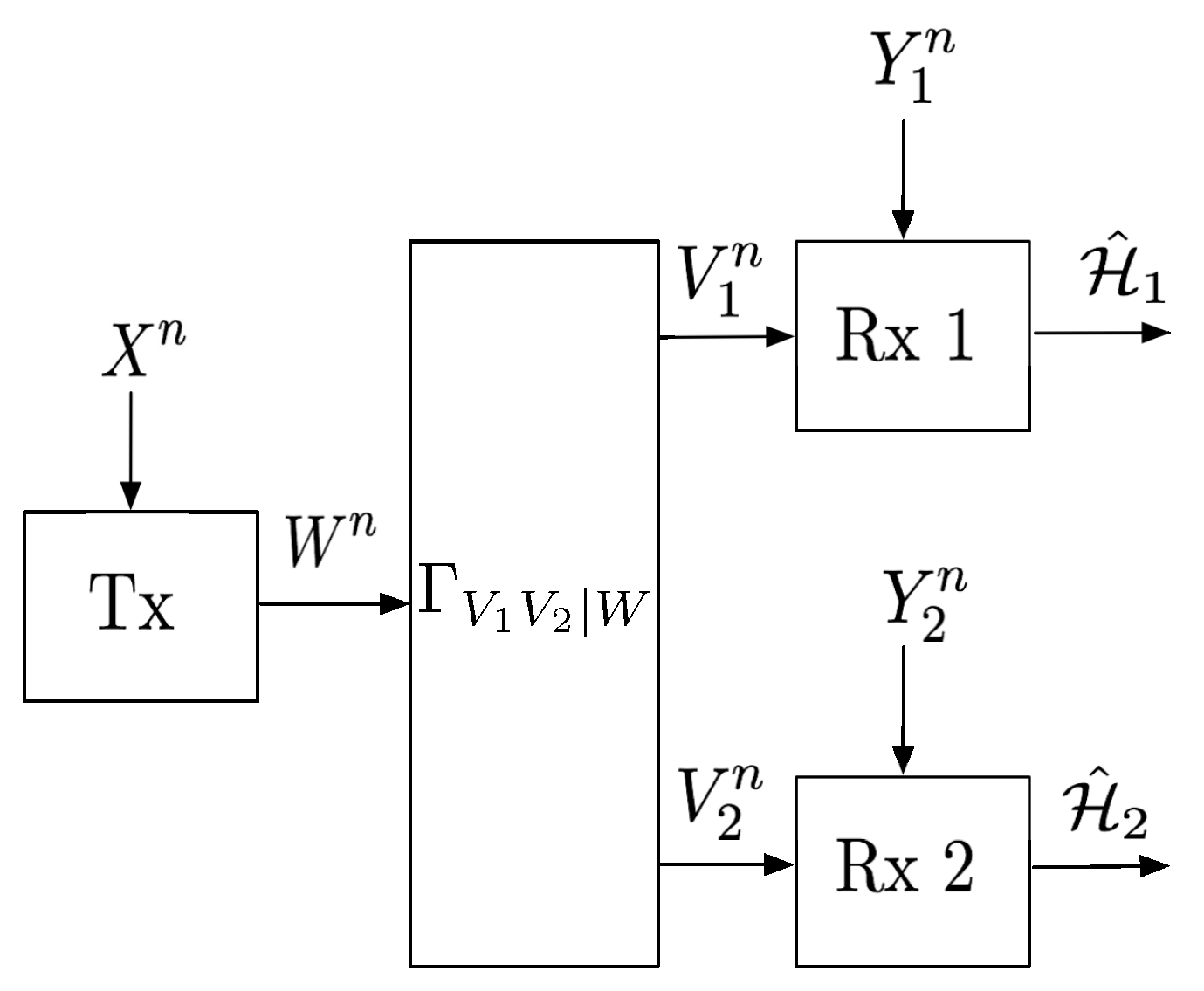
Consider the distributed hypothesis testing problem in Figure 1, where a transmitter observes sequence , Receiver 1 sequence , and Receiver 2 sequence . Under the null hypothesis:
and under the alternative hypothesis:
for two given pmfs and . The transmitter can communicate with the receivers over n uses of a discrete memoryless broadcast channel where denotes the finite channel input alphabet and and the finite channel output alphabets. Specifically, the transmitter feeds inputs
to the channel, where denotes the chosen (possibly stochastic) encoding function
Each Receiver observes the BC ouputs , where for a given input ,
Based on the sequence of channel outputs and the source sequence , Receiver i decides on the hypothesis . That means it produces the guess
for a chosen decoding function
There are different possible scenarios regarding the requirements on error probabilities. We assume that each receiver is interested in only one of the two exponents. For each , let be the hypothesis whose error exponent Receiver i wishes to maximize, and the other hypothesis, i.e., and . (The values of and are fixed and part of the problem statement.) We then have:
Definition 1.
An exponent pair is said to be achievable over a BC, if for each and sufficiently large blocklengths n, there exist encoding and decoding functions such that:
satisfy
and
Definition 2.
The fundamental exponents regionis the set of all exponent pairsthat are achievable.
Remark 1.
Notice that both and depend on the BC law only through the conditional marginal distribution . Similarly, and only depend on . As a consequence, also the fundamental exponents region depends on the joint laws and only through their marginal laws , , , and .
Remark 2.
As a consequence to the preceding Remark 1, when , one can restrict attention to a scenario where both receivers aim at maximizing the error exponent under hypothesis , i.e., . In fact, under , the fundamental exponents region for arbitrary and coincides with the fundamental exponents region for and if one exchanges pmfs and in case and one exchanges pmfs and in case .
To simplify the notation in the sequel, we use the following shorthand notations for the pmfs and .
For each :
and
We propose two coding schemes yielding two different exponent regions, depending on whether
or
3. Results on Exponents Region
Before presenting our main results, we recall the achievable error exponent over a discrete memoryless channel reported in [15] (Theorem 1).
3.1. Achievable Exponent for Point-to-Point Channels
Consider a single-receiver setup with only Receiver 1 that wishes to maximize the error exponent under hypothesis . For simplicity then, we drop the user index 1 and simply call the receiver’s source observation and its channel outputs .
Theorem 1
(Theorem 1 in [15]). Any exponent θ satisfying the following condition is achievable:
where the maximization is over pmfs , , and such that the joint law satisfies
and where the exponents in (15) are defined as:
Here, all mutual information terms are calculated with respect to the joint pmf defined above.
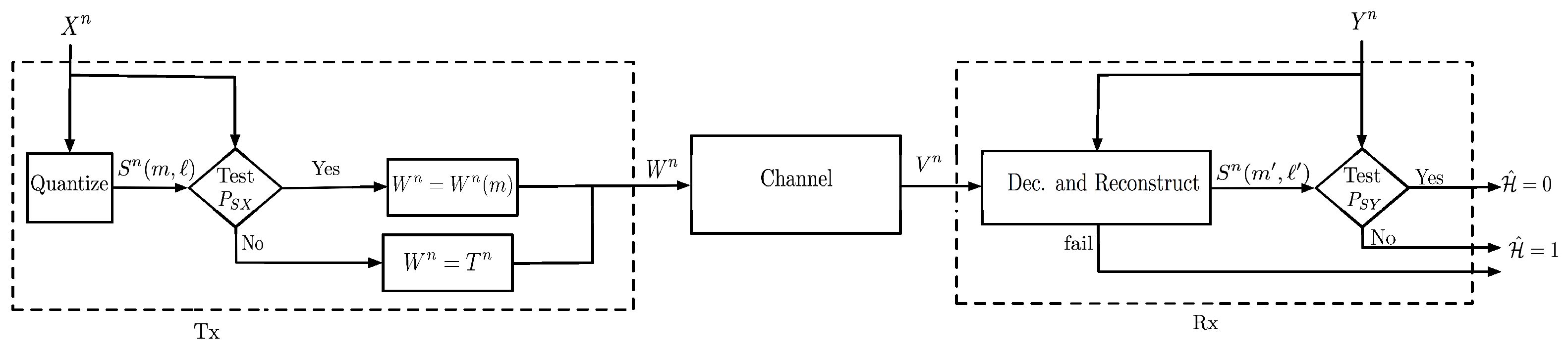
The exponent in Theorem 1 is obtained by the following scheme, which is also depicted in Figure 2.
The transmitter attempts to quantize the source sequence using a random codebook consisting of codewords . If the quantization fails because no codeword is jointly typical with the source sequence, then the transmitter applies the UEP mechanism in [17] by sending an IID -sequence over the channel. Otherwise, it sends the codeword for m indicating the first index of the codeword that is jointly typical with its source observation . The receiver jointly decodes the channel and source codeword by verifying the existence of indices such that is jointly typical with its channel outputs and there is no other codeword with smaller conditional empirical entropy given than . If the decoded codeword is jointly typical with the receiver’s observation , then it produces , and otherwise .
The three competing type-II error exponents in Theorem 1 can be understood in view of this coding scheme as follows. Exponent indicates the event that a random codeword is jointly typical with the transmitter’s observation and with the receiver’s observation while being under . This is also the error exponent in Han’s scheme [2] over a noiseless communication link and does not depend on the channel law . Exponent is related to the joint decoding that checks the joint typicality of the source codeword, as well as of the channel codeword, and applies a conditional minimum entropy decoder. A similar error exponent is observed in the SHA scheme [3,4] over a noiseless link if the mutual information is replaced by the rate of the link. The third exponent finally indicates an event where the transmitter sends (so as to indicate the receiver to decide for ) but the receiver detects a channel codeword and a corresponding source codeword . This exponent is directly related to the channel transition law and not only to the mutual information of the channel and does not occur when transmission is over a noiseless link. Interestingly, it is redundant in view of exponent whenever because in this case the minimization in (18) evaluates to . In this special case, the exponent can also be shown to be optimal, see [15].
We now present our achievable exponents region, where we distinguish the two cases (1) and ; and (2) or .
3.2. Achievable Exponents Region When and
Theorem 2.
Proof.
See Appendix A. □
In Theorem 2, the exponent triple can be optimized over the pmfs , and and independently thereof the exponent triple can be optimized over the pmfs , and . The pmf is common to both optimizations. However, whenever the exponents and are not active, Theorem 2 depends only on , and , for , and there is thus no tradeoff between the two exponents and . In other words, the same exponents and can be attained as in a system where the transmitter communicates over two individual DMCs and to the two receivers, or equivalently each receiver achieves the same exponent as if the other receiver was not present in the system.
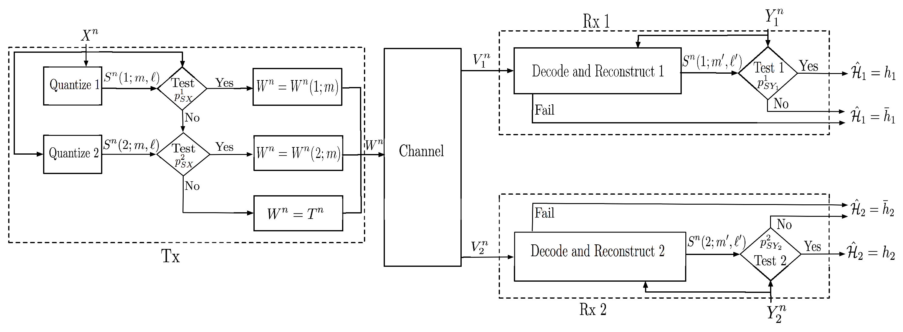
The scheme achieving the exponents region in Theorem 2 is described in detail in Section 4 and analyzed in Appendix A. The main feature is that the sensor makes a tentative decision on and conveys this decision to both receivers through its choice of the codebooks and a special coded time-sharing sequence indicating this choice. The receiver that wishes to maximize the error exponent corresponding to the hypothesis guessed at the sensor directly decides on this hypothesis. The other receiver should compare its own observation to a quantized version of the source sequence observed at the sensor. The sensor uses the quantization and binning scheme presented in [15] tailored to this latter receiver using either coded time-sharing sequence and codebooks and or coded time-sharing sequence and codebooks and , respectively. The overall scheme is illustrated in Figure 3.
Exponents , , and have similar explanations as in the single-user case. Exponent corresponds to the event that the transmitter sends a codeword from , for , but Receiver i decides that a codeword from was sent and a source codeword satisfies the minimum conditional entropy condition and the typicality check with the observed source sequence . Notice that setting as a constant decreases the error exponent .
3.3. Achievable Exponents Region for or
Define for any pmfs , and function
the joint pmfs
and
and for each , the four exponents
Theorem 3.
Proof.
The coding and testing scheme achieving these exponents is described in Section 5. The analysis of the scheme is similar to the proof of [15] (Theorem 4) and omitted for brevity. In particular, error exponent corresponds with the event that Receiver i decodes the correct cloud and satellite codewords but wrongly decides on . In contrast, error exponents and correspond to the events that Receiver i wrongly decides on after wrongly decoding both the cloud center and the satellite or only the satellite. Error exponent corresponds to the miss-detection event. Due to the implicit rate constraints in (46), the final constraints in (31) are obtained by eliminating the rates by means of Fourier–Motzkin elimination. Notice that in constraint (31c), the mutual information is multiplied by a factor 2, whereas in (31b), it appears without a factor. The reason is that the error analysis includes union bounds over the codewords in a bin and when wrongly decoding the satellite codewords (which is the case of exponents and ) then the union bound is over pairs of codewords, whereas under correct decoding, it is over single codewords. In the former case, we have the factor in the error probability, and, in the latter case, the factor . The auxiliary rates and are then eliminated using the Fourier–Motzkin elimination algorithm. □
For each , exponents , and have the same form as the three exponents in [15] (Theorem 1) for the DMC. There is, however, a tradeoff between the two exponents and in the above theorem because they share the same choice of the auxiliary pmfs and and the function f. In [10], the above setup is studied in the special case of testing against conditional independence, and the mentioned tradeoff is illustrated through a Gaussian example.
4. Coding and Testing Scheme When
Fix , a sufficiently large blocklength n, auxiliary distributions , and over , conditional channel input distributions and , and conditional pmfs and over a finite auxiliary alphabet such that for each :
The mutual information in (33) is calculated according to the joint distribution:
For each , if , choose rates
If , then choose rates
Code Construction: Generate a sequence by independently drawing each component according to . For each , generate a sequence by independently drawing each according to when . In addition, construct a random codebook
superpositioned on where the k-th symbol of codeword is drawn independently of all codeword symbols according to when and . Finally, construct a random codebook
by independently drawing the k-th component of codeword according to the marginal pmf .
Reveal all codebooks and the realizations of the sequences to all terminals.
Transmitter: Given source sequence , the transmitter looks for indices such that codeword from codebook satisfies
and the corresponding codeword from codebook satisfies
(Notice that when is sufficiently small, then Condition (41) can be satisfied for at most one value , because .) If successful, the transmitter picks uniformly at random one of the triples that satisfy (41), and it sends the sequence over the channel. If no triple satisfies Condition (41), then the transmitter sends the sequence over the channel.
Receiver : Receives and checks whether there exist indices such that the following three conditions are satisfied:
If successful, it declares . Otherwise, it declares .
Analysis: See Appendix A.
5. Coding and Testing Scheme When
In this case, the scheme is based on hybrid source-channel coding. Choose a large positive integer n, auxiliary alphabets , and , and a function f as in (27).
Choose an auxiliary distribution over , and a conditional distribution over so that for inequalities (32) are satisfied with strict inequality.
Then, choose a positive and rates so that
and
Generate a sequence i.i.d. according to and construct a random codebook
superpositioned on where each codeword is drawn independently according to conditioned on . Then, for each index and , randomly generate a codebook
superpositioned on by drawing each entry of the n-length codeword i.i.d. according to the conditional pmf where denotes the k-th symbol of . Reveal the realizations of the codebooks and the sequence to all terminals.
Transmitter: Given that it observes the source sequence , the transmitter looks for indices that satisfy
If successful, it picks one of these indices uniformly at random and sends the codeword over the channel, where
and where denote the k-th components of codewords . Otherwise, it sends the sequence of inputs over the channel.
Receiver : After observing and , Receiver looks for indices and that satisfy the following conditions:
If successful, Receiver i declares . Otherwise, it declares .
Analysis: Similar to [15] (Appendix D) and omitted.
6. Summary and Conclusions
The paper proposed and analyzed general distributed hypothesis testing schemes both for the case where the sensor can distinguish the two null hypotheses and where it cannot. Our general schemes recover all previously studied special cases. Moreover, our schemes illustrate a similar phenomenon for setups with common noisefree communication links from the sensor to all decision centers: while a tradeoff arises when the transmitter cannot distinguish the alternate hypotheses at the two decision centers, such a tradeoff can almost completely be mitigated when the transmitter can distinguish the alternate hypotheses. In contrast to the noise-free link scenario, under a noisy broadcast channel model, a tradeoff can still arise in this case because decision centers can confuse the decision taken at the transmitter, and thus misinterpret to whom the communication is dedicated.
Interesting directions for future research include information-theoretic converse results and extensions to multiple sensors or more than two decision centers.
Author Contributions
Author Formal analysis, S.S. and M.W.; writing—original draft preparation, S.S.; writing—review and editing, M.W. All authors have read and agreed to the published version of the manuscript.
Funding
Author has received funding from the European Research Council (ERC) under the European Union’s Horizon 2020 programme, grant agreement No 715111.
Conflicts of Interest
The authors declare no conflict of interest.
Appendix A. Proof of Theorem 2
The proof is based on the scheme of Section 4. Fix a choice of blocklength n, the small positive and the (conditional) pmfs , , , , , and so that (22) holds. Assume that and , in which case are given by (37) and (38). Additionally, set for convenience of notation:
The analysis of type-I error probability is similar as in [15] (Appendix A). The main novelty is that because for some , for sufficiently small values of , the source sequence cannot lie in both and . Details are omitted.
Consider the type-II error probability at Receiver 1 averaged over all random codebooks. Define the following events for :
Notice that
Above probability is upper bounded as:
The sum of above probabilities can be upper bounded by the sum of the probabilities of the following events:
Thus, we have
The probabilities of events , , and can be bounded following similar steps to [15] (Appendix A). This yields:
for some functions , , and that go to zero as n goes to infinity and , and where we define:
Consider event :
where holds because the channel code is drawn independently of the source code and holds by Sanov’s theorem.
Define
and notice that
for a function that goes to zero as and
Here, holds because the condition implies that and thus , and holds by the constraints in the minimizations.
By standard arguments and successively eliminating the worst half of the codewords with respect to and the exponents , , and , it can be shown that there exists at least one codebook for which
Letting and , we get , , and . A similar bound can be found for . This concludes the proof.
References
- Ahlswede, R.; Csiszár, I. Hypothesis testing with communication constraints. IEEE Trans. Inf. Theory 1986, 32, 533–542. [Google Scholar] [CrossRef] [Green Version]
- Han, T.S. Hypothesis testing with multiterminal data compression. IEEE Trans. Inf. Theory 1987, 33, 759–772. [Google Scholar] [CrossRef]
- Shimokawa, H.; Han, T.; Amari, S.I. Error bound for hypothesis testing with data compression. In Proceedings of the 1994 IEEE International Symposium on Information Theory, Trondheim, Norway, 27 June–1 July 1994; p. 114. [Google Scholar]
- Shimokawa, H. Hypothesis Testing with Multiterminal Data Compression. Master’s Thesis, University of Tokyo, Tokyo, Janpan, 1994. [Google Scholar]
- Weinberger, N.; Kochman, Y. On the reliability function of distributed hypothesis testing under optimal detection. IEEE Trans. Inf. Theory 2019, 65, 4940–4965. [Google Scholar] [CrossRef]
- Rahman, M.S.; Wagner, A.B. On the optimality of binning for distributed hypothesis testing. IEEE Trans. Inf. Theory 2012, 58, 6282–6303. [Google Scholar] [CrossRef] [Green Version]
- Zhao, W.; Lai, L. Distributed testing against independence with multiple terminals. In Proceedings of the 2014 52nd Annual Allerton Conference on Communication, Control, and Computing (Allerton), Monticello, IL, USA, 30 September–3 October 2014; pp. 1246–1251. [Google Scholar]
- Xiang, Y.; Kim, Y.H. Interactive hypothesis testing against independence. In Proceedings of the 2013 IEEE International Symposium on Information Theory, Istanbul, Turkey, 7–12 July 2013; pp. 2840–2844. [Google Scholar]
- Katz, G.; Piantanida, P.; Debbah, M. Collaborative distributed hypothesis testing with general hypotheses. In Proceedings of the 2016 IEEE International Symposium on Information Theory (ISIT), Barcelona, Spain, 10–15 July 2016; pp. 1705–1709. [Google Scholar]
- Salehkalaibar, S.; Wigger, M.; Timo, R. On hypothesis testing against independence with multiple decision centers. IEEE Trans. Commun. 2018, 66, 2409–2420. [Google Scholar] [CrossRef] [Green Version]
- Salehkalaibar, S.; Wigger, M.; Wang, L. Hypothesis testing over the two-hop relay network. IEEE Trans. Inf. Theory 2019, 65, 4411–4433. [Google Scholar] [CrossRef]
- Escamilla, P.; Wigger, M.; Zaidi, A. Distributed hypothesis testing with concurrent detection. In Proceedings of the 2018 IEEE International Symposium on Information Theory (ISIT), Vail, CO, USA, 17–22 June 2018. [Google Scholar]
- Escamilla, P.; Wigger, M.; Zaidi, A. Distributed hypothesis testing: Cooperation and concurrent detection. IEEE Trans. Inf. Theory 2020, 66, 7550–7564. [Google Scholar] [CrossRef]
- Tian, C.; Chen, J. Successive refinement for hypothesis testing and lossless one-helper problem. IEEE Trans. Inf. Theory 2008, 54, 4666–4681. [Google Scholar] [CrossRef] [Green Version]
- Salehkalaibar, S.; Wigger, M. Distributed hypothesis testing based on unequal error protection codes. IEEE Trans. Inf. Theory 2020, 66, 4150–4182. [Google Scholar] [CrossRef]
- Sreekumar, S.; Gündüz, D. Distributed hypothesis testing over discrete memoryless channels. IEEE Trans. Inf. Theory 2020, 66, 2044–2066. [Google Scholar] [CrossRef]
- Borade, S.; Nakiboglu, B.; Zheng, L. Unequal error protection: An information-theoretic perspective. IEEE Trans. Inf. Theory 2009, 55, 5511–5539. [Google Scholar] [CrossRef]
- El Gamal, A.; Kim, Y.H. Network Information Theory; Cambridge University Press: Cambridge, MA, USA, 2011. [Google Scholar]
Figure 1.
Hypothesis testing over a noisy BC.

Figure 2.
Coding and testing scheme for hypothesis testing over a DMC.

Figure 3.
Coding and testing scheme for hypothesis testing over a BC.

Publisher’s Note: MDPI stays neutral with regard to jurisdictional claims in published maps and institutional affiliations. |
© 2021 by the authors. Licensee MDPI, Basel, Switzerland. This article is an open access article distributed under the terms and conditions of the Creative Commons Attribution (CC BY) license (https://creativecommons.org/licenses/by/4.0/).
Share and Cite
MDPI and ACS Style
Salehkalaibar, S.; Wigger, M. Distributed Hypothesis Testing over Noisy Broadcast Channels. Information 2021, 12, 268. https://0-doi-org.brum.beds.ac.uk/10.3390/info12070268
AMA Style
Salehkalaibar S, Wigger M. Distributed Hypothesis Testing over Noisy Broadcast Channels. Information. 2021; 12(7):268. https://0-doi-org.brum.beds.ac.uk/10.3390/info12070268
Chicago/Turabian StyleSalehkalaibar, Sadaf, and Michèle Wigger. 2021. "Distributed Hypothesis Testing over Noisy Broadcast Channels" Information 12, no. 7: 268. https://0-doi-org.brum.beds.ac.uk/10.3390/info12070268
Note that from the first issue of 2016, this journal uses article numbers instead of page numbers. See further details here.