
Dynamic Optimal Travel Strategies in Intelligent Stochastic Transit Networks


Department of Enterprise Engineering, University of Rome Tor Vergata, 00133 Rome, Italy
*
Author to whom correspondence should be addressed.
Information 2021, 12(7), 281; https://0-doi-org.brum.beds.ac.uk/10.3390/info12070281
Submission received: 3 June 2021
/
Revised: 3 July 2021
/
Accepted: 9 July 2021
/
Published: 13 July 2021
(This article belongs to the Special Issue New Generation of Intelligent Transit Systems: Theory and Applications)
Abstract
:This paper addresses the search for a run-based dynamic optimal travel strategy, to be supplied through mobile devices (apps) to travelers on a stochastic multiservice transit network, which includes a system forecasting of bus travel times and bus arrival times at stops. The run-based optimal strategy is obtained as a heuristic solution to a Markovian decision problem. The hallmarks of this paper are the proposals to use only traveler state spaces and estimates of dispersion of forecast bus arrival times at stops in order to determine transition probabilities. The first part of the paper analyses some existing line-based and run-based optimal strategy search methods. In the second part, some aspects of dynamic transition probability computation in intelligent transit systems are presented, and a new method for dynamic run-based optimal strategy search is proposed and applied.
1. Introduction
The search for the best path on stochastic multiservice transit networks SMSTN (defined below) is no simple task compared with the case of regular service networks. This paper intends to contribute to solving this problem in the case of intelligent transit systems (ITS), with automated vehicle location (AVL) and at-stop bus arrival time forecasting, where apps (trip planners) are available on mobile devices, advising travelers of the best path to their destination [1,2,3,4].
According to [3] and focusing on schedule-based services (as motivated below), different studies pointed out the role of real-time information on path choice. For example, Reference [5] studied a case where the real-time information was relevant at the origin of the trip. Reference [6] studied the global pre-trip information based on the previous day and level of real-time information provided locally, but the effect of real-time information has not been studied in-depth since then. References [7,8] applied advanced public transport information systems with information on waiting times at stops and on-board crowding. References [9,10] evaluated the impact of different level of real-time information in Stockholm, while Reference [11] in Riviera (Uruguay). Reference [12] pointed out pre-trip real-time information also considering disruptions. Reference [13] contributed to the transit assignment literature by addressing personalization and bounded rationality. Thus, the need to equip users/travelers with mobile transit route planners that provide personal information [14,15] on origin–destination routes rather than to real-time information at stops or pre-. It envisions the creation of a better transportation experience. However, the framework presented in this paper can be applied both to the search for the best path in SMSTN (to be suggested by transit trip planners), and in transit assignment modelling for intelligent transit systems in which such a trip planner is used by travelers.
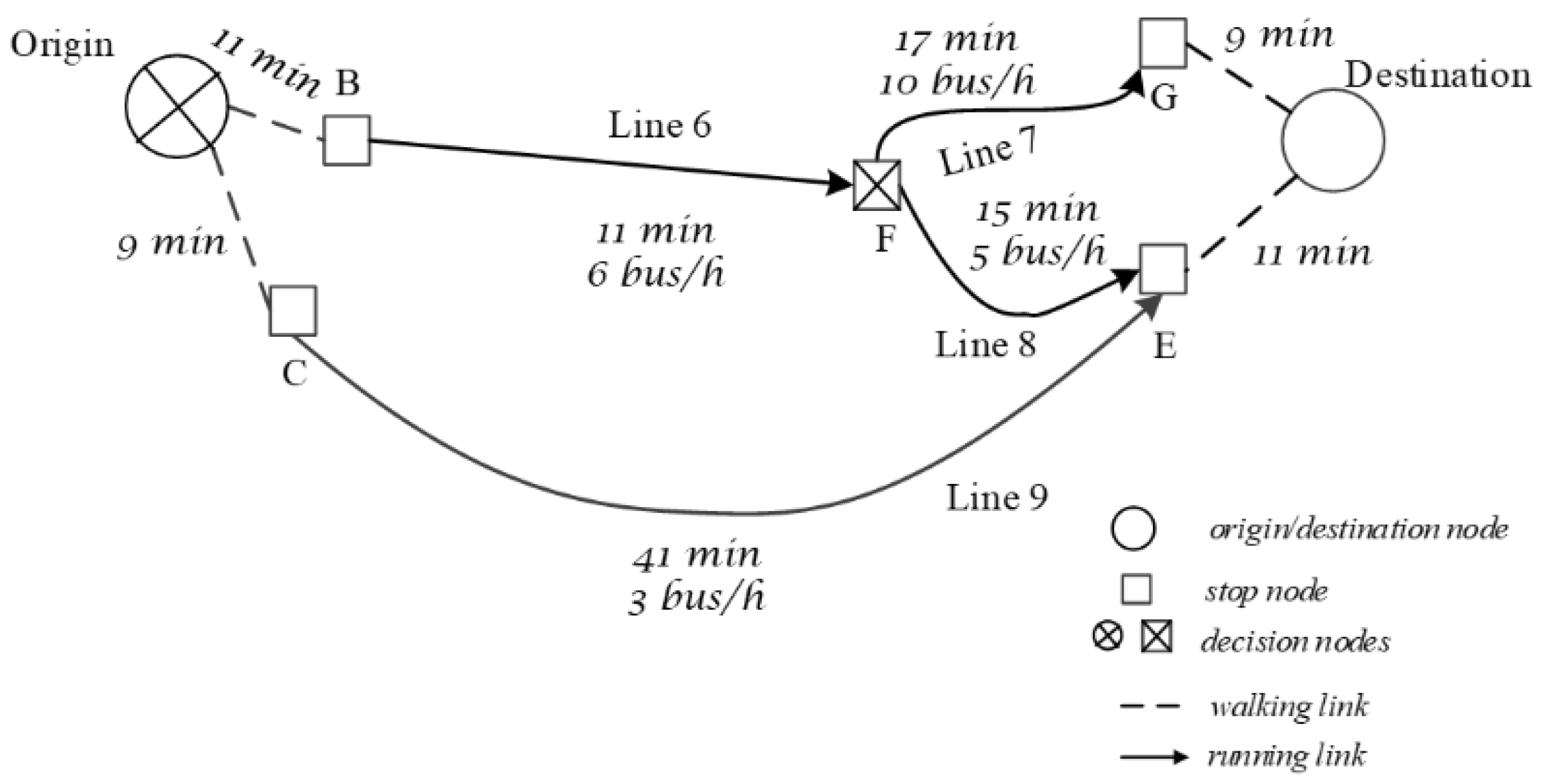
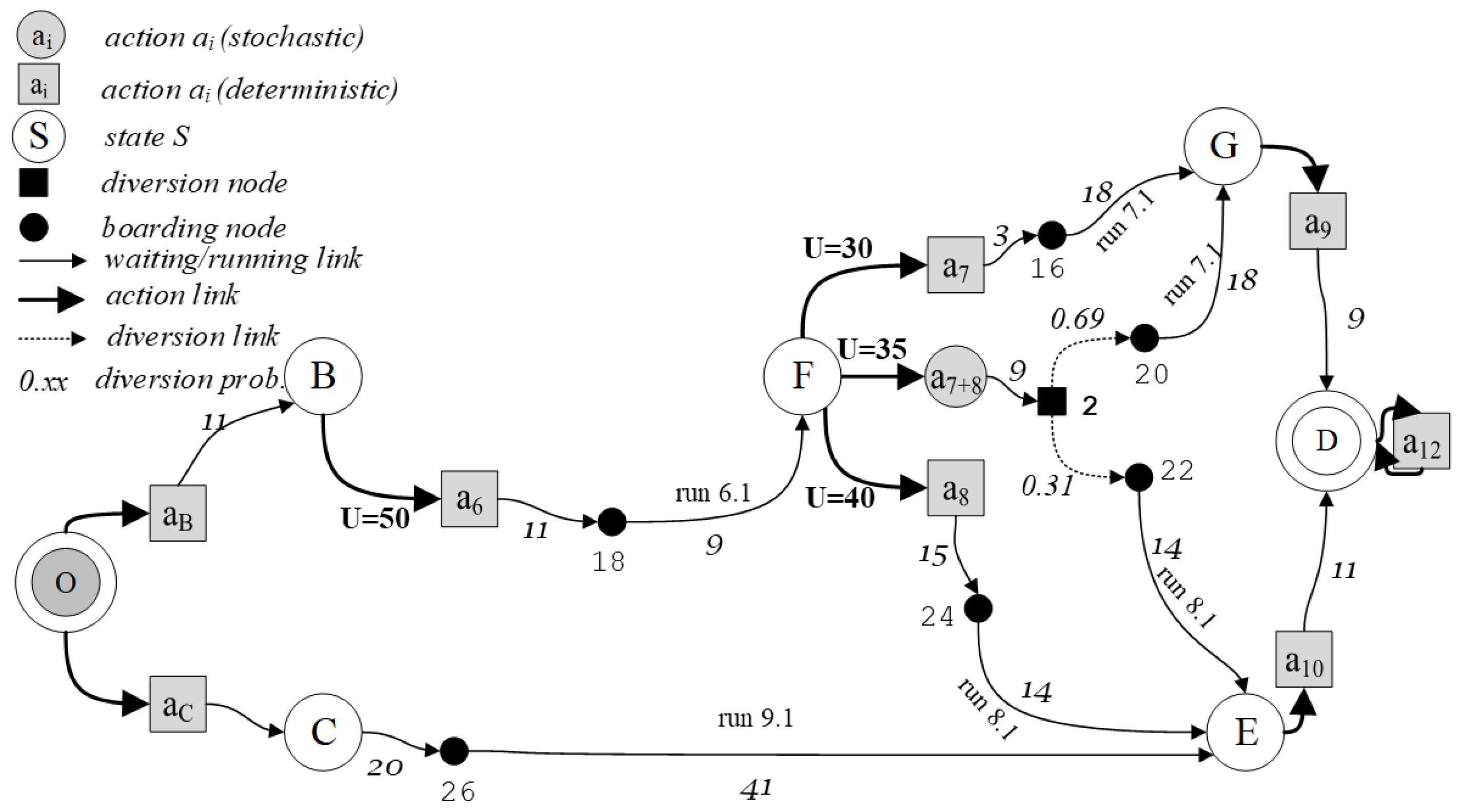
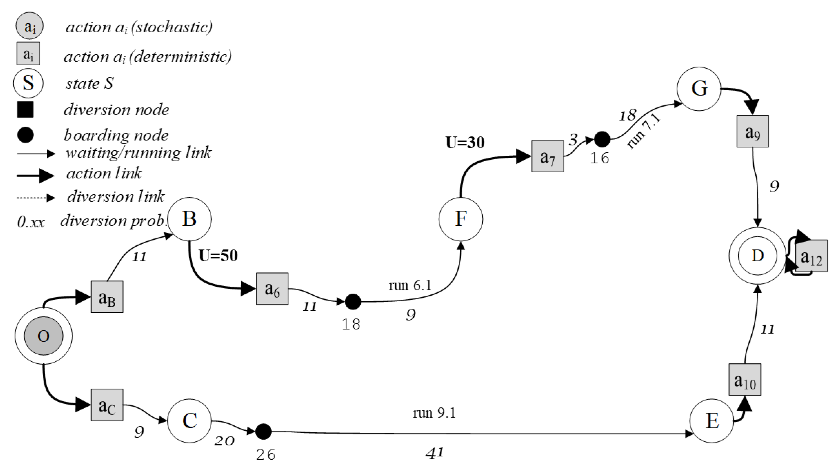
Given an origin–destination (O-D) pair on a transit service network N, let SGOD be the subgraph that includes the available line paths connecting the O-D pair. If more than one line is available to reach the destination at some bus stops, the network is classified as a multiservice transit network (MSTN). An example of a multiservice network is reported in Figure 1, where at node F two lines are available to reach destination D. If some path attributes X (e.g., waiting time, on-board time, on-board occupancy degree) are random variables, and MSTN is classified as a stochastic multiservice network (SMSTN). In the following, only ordinary randomness is taken into account. For example, effects due to large service disruptions are not considered.
In stochastic networks, actual bus arrival times may differ from those scheduled or forecasted. Because of stochasticity, the outcome of any decision depends partly on the agent’s decisions and partly on randomness. For example, in the network illustrated in Figure 1, the final outcome of the choice of line 6 at stop B also depends on what will happen when the traveler arrives at stop F and on the set of lines considered in that node. Therefore, in an SMSTN, an optimal path from origin to destination, found at the origin (a priori routing) on the basis of forecasted at-stop bus arrival times and suggested to a traveler, may include links il at nodes i that could prove non-optimal when the traveler arrives at the above nodes. An a priori optimal path, which includes line 7 at node F, forecasted as the first arriving line, could be suggested in a priori routing, but when the traveler arrives at F, line 8 could arrive first, thus becoming more convenient if it has the same or less forecasted travel time to destination. See also [16] on this topic. Thus, not a complete single O-D path should be suggested to travelers, but rather one optimal travel strategy.
A trip from origin to destination on a stochastic multiservice network can be represented in the decision theory (DT) approach as a sequence of decisions (decision process-DPs) at some diversion nodes (origin, first boarding stop, transfer stops) where sets of stops and lines may be available to continue the trip as far as the destination. Travelling from origin to destination, a traveler passes from a state St (a decision node) to another state St+1, depending on the action chosen and on the stochastic occurrences in St. The transition probabilities conditional upon an action “a” are the probabilities of going from a state St to each of the following states St+1 if action “a” is applied. Thus a trip from origin to destination on a stochastic network with diversion nodes is a stochastic decision process (SDPs). If the transition probabilities and the expected rewards depend only on state S and not on the previous transitions, the decision process is considered as decision-making in a Markov decision process (MDPs), and the Markov decision problem (MDPm) approach [17] can be used. MDPm problems can be more easily solved when the transition probabilities and the expected rewards are known through Bellman’s algorithms [18,19].
In an optimal travel strategy search, different approaches can be used. A more traditional approach, often reported as a line-based or frequency approach, considers bus services in terms of lines, with their service frequencies and average travel times, both assumed constant during a given time period.
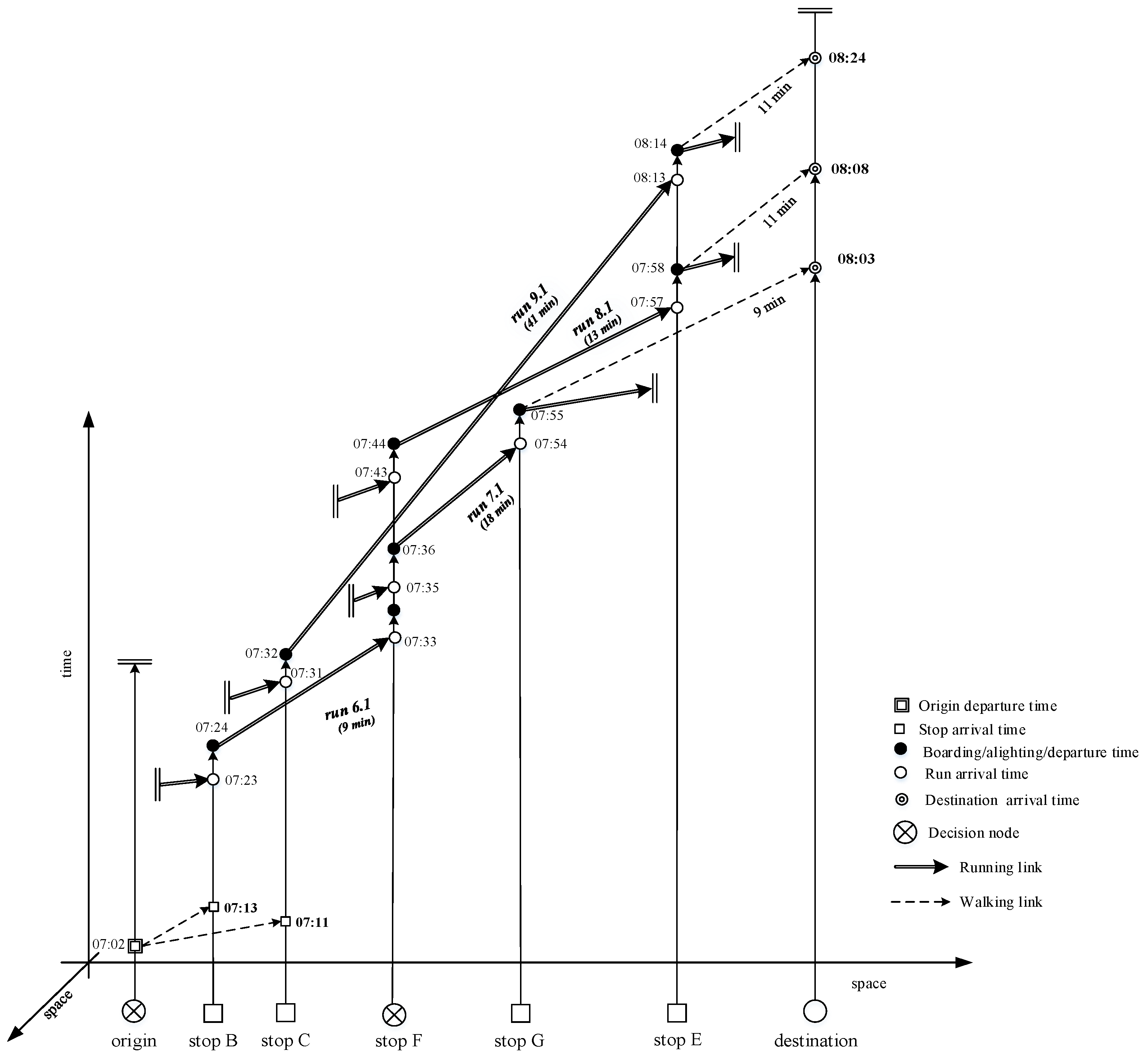
Some recent papers on optimal strategies consider a run-based (also in the literature bus-based or vehicle-based or schedule-based) approach with a service representation, in which each run of each line is explicitly considered through run-based or vehicle-based graphs [20,21,22,23,24,25] In a run graph, the nodes have coordinates in space and time and the services are defined in terms of single runs, with specific bus arrival and departure times at each stop (see, for example, Figure 6 in Section 5). In this approach, within-day and day-to-day time-dependent states of the stochastic service network and real-time forecasted information on future network states are taken into account.
One of the main differences between line-based and run-based search for optimal strategies is that, in the latter case, the number of possible states grows dramatically if all the states of each traveler and of each bus are considered. Due to the large number of states, the search methods inherit the curse of dimensionality, and therefore state–space reduction through pre-processing has been proposed and applied (see for example [16]).
In the field of run-based optimal strategy searches, this paper proposes a new heuristic search method, which seeks to limit the number of states and computes the transition probabilities using a real-time error distribution of bus travel time forecasts and at-stop bus arrival time forecasts. The method is suitable for intelligent transit systems as well as to be implemented in apps for providing route guidance in SMSTN since it includes a forecasting system for bus travel times and arrival times at stops.
In the following, using the notation described in Table 1, Section 2 considers the search methods of optimal travel strategies for the line-based approach, while in Section 3 the bus-based or run-based approach, presented in the literature, is recalled. An analysis of the forecasting error of bus at-stop arrival times, used in the proposed method, is reported in Section 4. The newly proposed search method is presented in Section 5, with an example of its application in Section 6. Finally, Section 7 outlines some comments and draws conclusions.
2. The Line-Based Search of an Optimal Travel Strategy
In this section, the line-based search for optimal strategies is recalled, in order to highlight the main differences with the run-based approach, as analyzed in Section 3.
User optimal path searches in stochastic multiservice transit networks have been studied since the 1970s (see for example [26]) and the main research strand applies decision theory [27], especially stochastic decision theory [17]. Because of the stochasticity of the services, the choices entail decision-making without comprehensive knowledge of all relevant factors and their possible future evolution. Thus, as reported in the Introduction, no complete a priori single origin–destination path should be followed by travellers, but rather one specific set of lines (an attractive set), in each decision node, has to be potentially usable in order to optimize traveller choices in the long term. In relation to the outcomes at the decision node, one of the above lines is chosen, applying a rule that minimizes the expected travel time to destination. The sequence of attractive sets that minimizes the decision maker’s expected travel time is the optimal decision policy, in our case, the optimal travel policy or the optimal travel strategy. Each attractive line set is called an action in decision theory and therefore, an optimal strategy is an optimal sequence of actions, that is of attractive line sets.
2.1. State–Action Tree Representation of a Decision Process (DP)
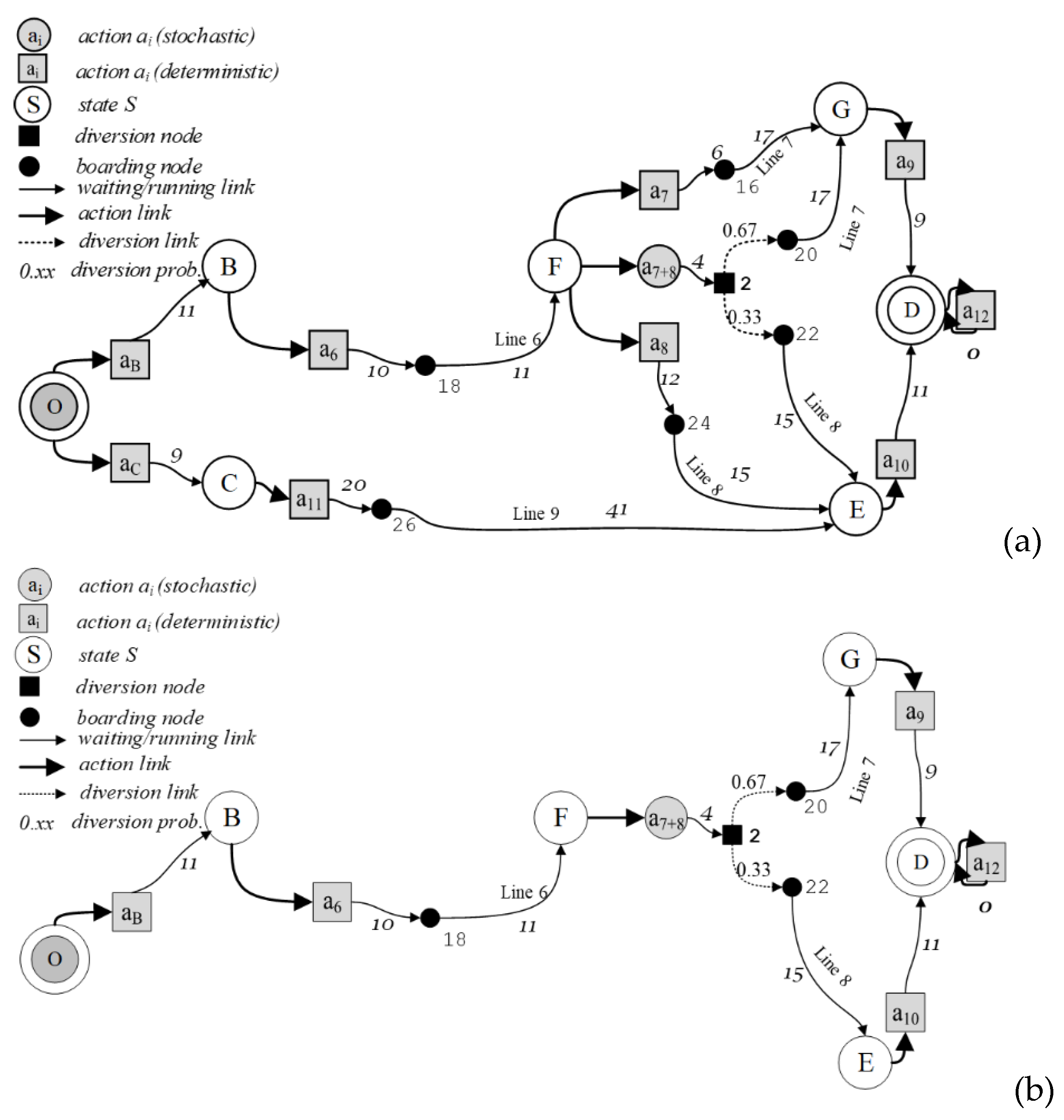
A MDPm can be represented through a state–action tree of the decision process. At every decision node, each possible action includes a set of outgoing links to the next decision nodes. For example, for the service line graph in Figure 1, at decision node F three different actions are possible, as represented in Figure 2a: (1) to use only line 7 (action a7); (2) to use only line 8 (action a8); (3) to consider lines 7 and 8 (action a7+8), comparing the expected travel time of each alternative action and then choosing the best one.
Given a state–action tree, different combinations of action sequences are possible. For the state–action trees in Figure 2a, examples of policies from node B, considering only states with transition probabilities different from zero, are as follows:
- (B, a6); (F, a7); (G, a9); (D, a12);
- (B, a6); (F, a8); (E, a10); (D, a12);
- (B, a6); (F, a7+8); (G, a9); (E, a10); (D, a12).
The expected reward raj(si, si−1) of state si, conditional upon the previous state si−1 and action aj, is in our case the expected travel cost of arriving in si from si−1 with aj.
2.2. Line-Based Transition Probabilities
When only one state corresponds to an action, the result of the action is deterministic and the transition probability to that state is 1, while to the other states, it is zero. When more than one state can follow an action, with some transition probabilities different from 0, the result of the action is stochastic. For example, in Figure 1, if at node F action a7 is applied, only node G can follow, with a probability equal to 1. The same holds for deterministic action a8 and node E. If at node F action a7+8 is applied, the transition probability of moving onto node G is equal to the probability that, when the traveler observes the system state and makes a decision at node F, the expected travel time of choosing line 7 is better than that of line 8, and hence line 7 is chosen. In the same way, the transition probability of moving onto node E is equal to the probability of line 8 being chosen. The transition probabilities are represented through a matrix. For example, given the policy: (O, aB); (B, a6); (F, a7+8); (G, a9); (E, a10); (D, a12), and its state–action tree (Figure 2b), the line-based transition probability matrix is reported in Table 2.
2.3. Transition Probability Determination in the Line-Based Approach
As stated above, an MDPm can be more easily solved, if the transition probabilities and the expected rewards are known, by applying Bellman algorithms [18]. Therefore, in this section, some methods applied in the line-based (or frequency-based) approach to obtain the transition probabilities are recalled and analyzed.
With a line-based representation of the service, the simplest way to obtain transition probabilities directly or indirectly is to assume that transit services are completely irregular, and the decision-maker has no information on current service states, but she/he only knows the average line waiting and travel times, and no capacity constraint exists. Action at each decision node consists of considering a subset of suitable lines for the destination, boarding the first arriving one. Transition probabilities pi and average waiting times wi are evaluated not in relation to single bus states, but directly in relation to the line frequencies (φi): pi = φi/(Σjφj); wi = 1/(Σjφj).
To solve the relative MDPm, [28,29] used a linear programming approach. Reference [30] highlighted the underlying graph structure of Spiess’ basic strategy concept, introducing a graph-theoretic framework and the concept of hyperpath and proposed a shortest hyperpath algorithm, using the generalized Bellman equations to obtain the optimal strategy. For example, using boarding stop B reported in Figure 1, the optimal hyperpath in Figure 3 corresponds to the optimal policy, obtained with a Bellman’s backward induction algorithm.
An example of a transit trip planner which uses this approach is HYPERPATH [31]. A set of attractive lines is indicated for the following stops of the path and the traveller is advised to board the first arriving line.
3. Optimal Travel Strategy Search in a Run-Based Approach
Run-based (or bus-based) search for an optimal travel strategy is quite a recent topic of transit path choice, hence generating relatively few papers in the literature.
Reference [16] refer to the adaptive transit routing (ATR) problem, formally defined as follows: “given a stochastic transit network (in which the transit travel times are time-dependent and random with known distributions), the initial state of the system and a destination D, an adaptive policy that minimizes the total expected travel time is sought, subject to a constraint that D is reached within a threshold TH with probability 1”. They present a method to solve an adaptive routing problem with link travel times that are discrete random variables with known probability distributions. The authors consider the bus state space and the traveller state space. Given a system–state space, the action space is the set of actions available to a traveler at different stops and the possible alternatives can be: board, wait, or walk to another stop. Because of the large number of states, the method inherits the curse of dimensionality, and therefore state–space reduction through pre-processing is proposed and applied.
In a transit route planner context, [34] apply time-dependent routing advice that specifies a set of services at each location, from which the traveler is recommended to take the one that arrives first. The authors show that an optimal policy may not always exist and two heuristic solutions for finding a ‘good’ current time-dependent policy are proposed.
4. Analysis of the Forecasting Error of Bus At-Stop Arrival Times
This paper proposes a data-driven method to determine transition probabilities which uses, as will be examined below, the probability distribution of run arrival time forecasting error εSy:
where is the actual run arrival time at stop Sy and is the forecasted value when the traveller is at stop Sx.
An experimental probability law of the forecasting errors can be estimated by collecting a sample of forecasted run arrival times and of actual arrival times for each line of the service network. Therefore, the method is suitable for intelligent transit systems including a forecasting system of bus travel times and at-stop bus arrival times.
In this section, based on an experimental survey, an analysis is performed of forecasting errors for bus travel times and arrival times at stops. The analysis considers the probability law of the forecasting error and, for reasons that will be explored in the following sections, the relationship between the forecasting error standard deviation and the forecast horizon, that is, the travel time from the node where the forecast is made to the node for which the arrival time is forecasted. The analysis was carried out using data collected from the bus service network of Rome, considering several sections of a line operating in the city [35,36].
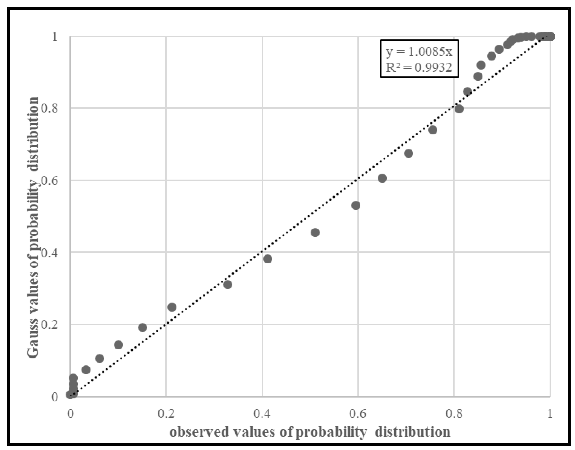
The forecasts of bus travel times (FTT) and arrival times at stop (FAT) can be obtained through several methods [37]. In this analysis, a time series method was applied, especially the STL—seasonal and trend decomposition using loess method [38], implemented in R software [39]. In order to obtain the probability law of the forecasting errors, comparisons among observed and normal error distributions were carried out. Figure 4 reports, as an example, the results obtained for one of the terminal-to-terminal sections, with a length of 11 km and using 2705 travel time measurements on weekdays. According to the Kolmogorov–Smirnov test (0.085; p-value = 0.14), there is probabilistic evidence that the forecasting errors were drawn from a normal distribution with zero mean and standard deviation equal to 263.80 s.
Using a set of different stop-to-stop distances, the empirical relationship of Figure 5 between error standard deviation and forecasting horizon was obtained. It shows an almost linear relation, with an increase in standard deviation when the forecasting horizon increases:
where:
- is the standard deviation (in seconds) of random forecasting error ε;
- FH is the forecasting horizon (in minutes).
Figure 5.
Empirical relation between standard deviation and forecasting horizon.

Such a result is consistent with similar empirical studies developed around the world both for transit services and private transport [40,41,42,43,44]. Thus, the error vector εSy, with a number of an element equal to the number of runs n at stop Sy, will be assumed below to be distributed according to a multivariate normal (MVN) with zero mean, dispersion matrix Σ and density probability given by:
5. The Proposed Run-Based Search Method of Dynamic Optimal Strategies
5.1. General Description of the Method
The proposed run-based search method applies a procedure that starts with the determination of a line-based feasible service network, that is a subnetwork of the original one, in which a set of feasible line paths is determined through some feasibility rules, such as: maximum number of line interchanges, maximum walking distance, maximum number of first boarding stops and last alighting stops, arrival time to destination in relation to the desired one. A line graph is thereby obtained with origin, some potential first boarding stops, some potential transfer stops, some potential last alighting stops and the destination, connected through pedestrian and transit links, as represented in Figure 1. The reduction of the initial network to feasible network has several advantages, not only in terms of paths actually used by travellers, but also in terms of reduction of problem dimension.
In this feasible network, decision nodes are the origin node and alighting stop nodes where a decision can be taken whether to stay there to board a run serving the stop or to walk to other boarding stops, choosing the alternative with the minimum expected travel time (or in general minimum expected travel disutility) to destination.
The proposed method follows a quite common procedure in dynamic ATR (see, for example [32]): at a decision node, the optimal strategy is searched with the information available at that node and the chosen optimal strategy is followed to the decision node downstream, where a new optimal strategy is searched using updated information.
At time t, when the traveler is at a decision node, a run-based (as stated above, in the literature also bus-based, vehicle-based or schedule-based) representation of the feasible network is generated from the decision node to the destination, using as temporal coordinates of the stops, the forecasted bus arrival times in these nodes, in turn, derived from stop-to-stop bus travel time forecasting. Hence, we can also refer to run-based travel strategies, to run hyperpaths, and to run-based transition probabilities. An example of a run-based representation of transit services relative to node B, when the traveler is at origin O at time to and therefore, the forecasts are carried out at to, is shown in Figure 6.
The proposed method searches the optimal strategy as a solution to an MDPm, based on the following criteria and assumptions:
- the traveller state space includes only decision nodes;
- when the traveller moves on the next decision node, a new optimal strategy is searched, considering the new forecasts of at-stop bus arrival time (FATS) and at-destination arrival times (FATD) available in real time. Therefore, each new optimal strategy is conditional upon the forecasts available at the current decision node;
- the bus state space is not considered, as better analysed in the following part of the paper, and hence the transition probabilities concern only transitions of the traveller between decision nodes;
- as an expected reward, the forecasted travel time (or, in general, the forecasted travel disutility) is used. Thus the optimal policy determines the combination of actions with minimum forecasted travel time up to destination. Therefore forecasting methods have to be used with expected value of FAT:E[FAT] = AT;
- considering the analysis results reported in Section 4, the forecasted arrival times FSxATSx at stop Sy forecasted when the traveler is at stop Sx can be expressed as follows:where is the true value of the arrival time at Sy and εSy is the forecasting error vector with known MVN probability density functions;
- all the buses are assumed to have unlimited capacity.
5.2. Run-Based Transition Probabilities
As stated above, in order to obtain the optimal strategy at a decision node using the MDPm approach, the method presented determines the traveller transition probabilities at downstream diversion nodes in relation to possible outcomes of bus arrival times at these downstream stops and to their forecasted arrival times at destination. For example, suppose that the traveler is at origin O of the run-based network in Figure 6, and the expected reward is searched deriving from the use of the policy including the stop B, the run 6.1 and then at stop F the action including the use of run 7.1 or of run 8.1. The current transition probabilities from node F to nodes E and G have to be determined in relation to the possible outcomes of arrival times and forecasted at-destination arrival times of run 7.1 and run 8.1 at stop F.
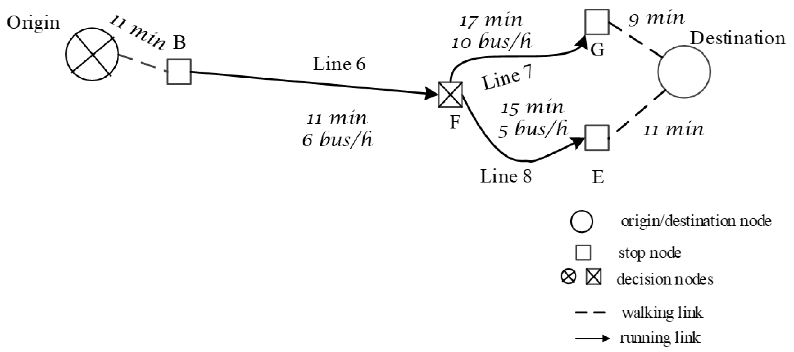
The model is formulated below for the case of a feasible service network with paths including at most only one interchanging stop JY (Figure 7). This is a very frequent case, because, even if a higher number of interchanges could actually exist, in general a feasible path with more than one interchanging stop is rarely used.
In the following, the transition probabilities are determined by considering the most complex case that the traveler is at node origin O at time to (see Figure 7). The optimal travel strategy from a first boarding stop I up to destination D, at time to, is searched. From stop I some runs RI1 … RIY … RIN lead to the decision stops J1, … JY, … JN, where some runs RJ1, RJ2, …, RJY…, RJM lead to the last alighting stops SJ1, SJ2, …, SJY…, SJM. If a larger number of lines is available between two stops, all their runs can be considered as runs of one equivalent line connecting the two stops.
The generic transition probabilities p[SJYY/I] for the time to can be obtained as:
where is the transition probability of moving from the decision node JY to stop SJYY, and p[JY/I] is the transition probability of moving from the decision node I to stop JY.
The transition probability p[SJYY/JY] is equal to the probability that, when the traveler will be at JY, the run RJYY, which arrives downstream at stop SJYY, is chosen. Remember that, as reported in Section 4, the forecasted at-stop arrival times are time-dependent random variables. Therefore, the forecasted bus arrival times at destination provided at stop JY could differ from those provided at origin O at to and the probability of boarding each run RJY at stop JY has to be estimated. The probability of boarding run is equal to the probability that, when the traveler is at boarding stop JY, the forecasted arrival time , at destination D, using run and forecasted at JY, is less than or equal to the, also forecasted at JY, arrival time at destination D, using one run RJY among the other runs RJ1, …, .
Therefore, the transition probability, , is:
where is the run choice set at stop JY, considered by the policy action in question.
As such transition probabilities are computed when the traveler is at origin O, the arrival times at destination D forecasted in JY have to be expressed as functions of the arrival times at destination forecasted at origin O. Let:
- be the true value of the arrival time at destination D using run ;
- be the arrival time at destination D using , forecasted at JY:where is the forecasting error;
- be the arrival time at destination D using run , forecasted at origin O:where is the forecasting error.
From the two above Equations (4) and (5), it follows that:
Similarly, the travel time at destination D forecasted at origin O by other runs can be obtained:
Finally, Equation (3), which gives the probability of moving from JY to computed when the traveller is at origin O, as the probability of choosing , is:
Considering also the results reported in the previous Section 4, the generic forecasting errors υj (i.e., linear combination of ε and η) can be assumed Multivariate Normal (MVN) random variables with zero mean () and n × n dispersion matrix Σ, where n is the number of alternative runs. Thus, forecasted arrival times FATj are also jointly distributed according to a multivariate normal distribution with mean vector actual arrival times (AT) and variances and co-variances equal to those of the residuals υj, FAT ~ MVN(AT, Σ).
The probability that a traveler will move from stop JY to stop is given by:
There is no known closed-form solution of the integral (Equation (9)) and numerical integration methods are to be applied. Besides, the MVN density probability of Equation (9) is quite complex to obtain for a large transit network. In order to simplify, it can be assumed that the forecasting errors are independently and identically distributed (i.i.d.) as a normal random variable with zero mean and variances . Thus, under such an assumption, the transition probabilities can be now computed as follows:
where W = is a normal random variable with zero mean and variance equal to the sum of variances of the above random errors.
The transition probability p[JY/I] of moving from the decision node I to stop JY can be computed in a very similar way, obtaining:
where:
- is the probability of boarding run at node I for reaching stop JY;
- is the arrival time at node JY using run at stop I forecasted at origin O;
- is the arrival time at node JY using run at stop I forecasted at origin O;
- are the forecasted errors.
Considering the approximations applied in the transition probabilities computation, the proposed search method, as stated above, has to be considered a heuristic method, with the advantages of strongly simplifying the real applications.
6. An Example of Dynamic Strategy Search Applying the Proposed Method
In this section, the proposed method is applied to the networking Figure 1 in a dynamic run-based strategy search. Figure 8 synthesize the modelling steps as described in the earlier sections.
At origin O, the optimal strategy using the first boarding stop B and the one using the first boarding stop C can be determined with reference to the run-based graph of Figure 6, obtained with the forecasts bus arrival times at stop available at the traveler’s departure time from the origin, and the corresponding state–action trees in Figure 9.
For the optimal strategy of boarding stop B the transition probabilities p[G/F] and p[E/F] have to be determined. The probability of moving from F to G computed when the traveler is at origin O can be calculated by applying Equation (8) and using the experimental relation between standard deviation and forecasting horizon reported in Equation (1) in Section 4 above. Thus, the estimates of the forecasting error variances, reported in Table 3, can be used.
From Equation (8), it follows that:
with Z standard normal random variable. Hence, the transition probability p[G/F] from F to G is about 0.69 and p[E/F] from F to E is about 0.31.
The numbers that in Figure 9 follow the action number aj are the forecasted transfer times from a run to the interchanging run. In the case of actions including more than one line, they are obtained as forecasted waiting time, weighted with the probabilities of use of each interchanging run, in our case, given by the transition probabilities.
By applying a Bellman algorithm, the optimal policy using boarding stop B reported in Figure 10 can be found.
For the first boarding stop C, as there are no decision nodes downstream, only one path is available, and the expected travel time to destination ca be directly determined by using the forecasted arrival time at destination D.
The optimal strategies via the first boarding stop B and the first boarding stop C are reported in Figure 10. It results that the absolute optimal strategy at origin is that related to boarding stop B, which allows earlier at destination D.
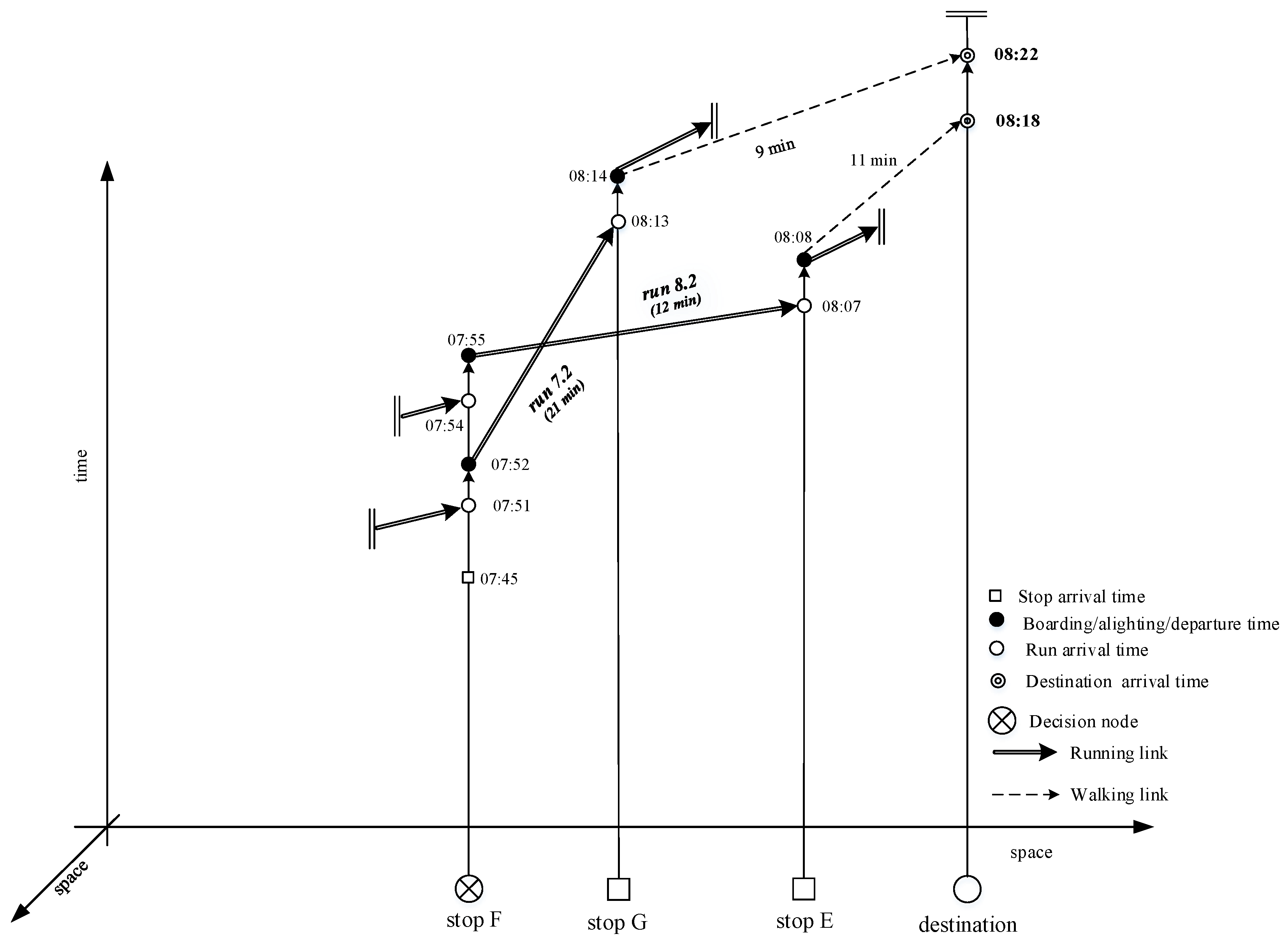
When a traveler is at stop F, the run graph of Figure 11 has to be considered, with the forecasted arrival times at destination via run 7.2 and run 8.2 (note that these times differ from that forecasted at origin O, due to the stochasticity of the services). The arrival time at destination of the first arriving run 7.2 is compared with the corresponding time of run 8.2, which had not yet arrived. In this case, waiting for run 8.2 is the best choice to make.
7. Conclusions
A heuristic search method was proposed in the context of a run-based optimal strategy search for stochastic multiservice transit networks. The method determines the optimal strategy as a solution of a Markovian Decision Problem and, in order to reduce the course of dimensionality, explicitly considered only the traveler states. As expected rewards, the forecasted travel times were used and the transition probabilities were obtained considering an empirical probability distribution of bus travel time forecasts and an empirical relationship between the forecasting horizon and its dispersion. The method is therefore suitable for intelligent transit systems, including a forecasting system of bus travel times and of arrival times at stops. The method was applied with satisfying results to a small test network.
The results indicate that personalized and predictive information, which is robust to varying data availability and can be provided with sufficient accuracy, can be useful to travelers for improving their travel experiences. In fact, the use of mobile applications (apps) to acquire real-time and readily available journey planning information is becoming instinctive behavior by public transport (PT) users. Through these mobile devices, the traveler does not only seek a path from origin to destination, but a satisfactory path that improve his/her travel experience. At the current stage of the telematics maturity and evolution, such a method can be implemented in available transit planners (apps) and could be a great lever for improving perception of effective services as well as to move people towards transit. However, some issues germinate from its complexity and the opportunity to update model parameters (e.g., travel time probability distribution). A preliminary desk comparison with other studies (e.g. [16]) allows us to assume that, as the presented method reduces the number states considering only feasible paths and traveler states, the computational complexity is largely reduced. However, such statements need to be validated in real and large transit networks. Then, it could be satisfactorily implemented into mobile transit route planners that provide information to travelers on origin–destination routes rather than to real-time information at stops, contributing as said to improve the attractivity of transit service. Therefore, the method is of value for agencies and operators in order to increase the attractiveness and capacity utilization of public transport, as well as for travelers in order to improve their travel experience limiting the impact of stochasticity of travel times, in particular with services that share the way and move on highly congested network.
The presented research can be extended in several directions. An area of further work is to evaluate whether more elaborated prediction methods can increase performance as well as how the probability distribution of travel time forecasts and an empirical relationship between the forecasting horizon and its dispersion may be easy to obtain through machine learning techniques. In particular, methods that can incorporate possible non-linear effects as well as multivariate correlations between loads, possible alighting counts at adjacent stops, and flows. Predictions under abnormal conditions such as special events, disruptions etc., is a particular area where novel modelling approaches may be required. Prediction accuracy for the probability of getting a seat upon boarding may be increased by solving it by data-driven approaches.
Another direction for extension is to explore the potential of historical and real-time data for personalized advising, which takes into consideration the users’ attitudes to boarding particular services.
Finally, several research issues still need to be resolved. These include, as mentioned, the application on larger test networks and real networks, and the development of methods based on a decision theory approach within theories other than that of expected utility.
Author Contributions
Conceptualization, A.N.; methodology, A.N. and A.C.; formal analysis, A.N. and A.C.; investigation, A.C.; data curation, A.C.; writing—original draft preparation, A.N. and A.C.; writing—review and editing, A.C.; supervision, A.N. and A.C.; funding acquisition, A.C. Both authors have read and agreed to the published version of the manuscript.
Funding
This research received no external funding. The APC was funded by MDPI.
Institutional Review Board Statement
Not applicable.
Informed Consent Statement
Not applicable.
Data Availability Statement
Not applicable.
Acknowledgments
The authors wish to thank the anonymous reviewers for their suggestions, which were most useful in revising the paper.
Conflicts of Interest
The authors declare no conflict of interest.
References
- Gentile, G.; Nguyen, S.; Pallottino, S. Route choice on transit networks with online information at stops. Transp. Sci. 2005, 39, 289–297. [Google Scholar] [CrossRef] [Green Version]
- Fonzone, A.; Schmöcker, J.-D. Effects of transit real-time information usage strategies. Transp. Res. Rec. 2014, 2417, 121–129. [Google Scholar] [CrossRef]
- Paulsen, M.; Rasmussen, T.K.; Nielsen, O.A. Impacts of real-time information levels in public transport: A large-scale case study using an adaptive passenger path choice model. Transp. Res. Part A Policy Pract. 2021, 148, 155–182. [Google Scholar] [CrossRef]
- Xiong, C.; Shahabi, M.; Zhao, J.; Yin, Y.; Zhou, X.; Zhang, L. An integrated and personalized traveler information and incentive scheme for energy efficient mobility systems. Transp. Res. Part C Emerg. Technol. 2020, 113, 57–73. [Google Scholar] [CrossRef]
- Hickman, M.D.; Wilson, N.H. Passenger travel time and path choice implications of real-time transit information. Transp. Res. Part C 1995, 3, 211–226. [Google Scholar] [CrossRef]
- Wahba, M.M. MILATRAS: MIcrosimulation Learning-Based Approach to TRansit ASsignment. Ph.D. Thesis, Department of Civil Engineering, University of Toronto, Toronto, ON, Canada, 2008. [Google Scholar]
- Comi, A.; Nuzzolo, A.; Crisalli, U.; Rosati, L. A New Generation of Individual Real-time Transit Information Systems. In Modelling Intelligent Multi-Modal Transit Systems; Nuzzolo, A., Lam, W.H.K., Eds.; CRC Press: Boca Raton, FL, USA, 2017; Chapter 3; pp. 80–107. [Google Scholar]
- Nuzzolo, A.; Crisalli, U.; Comi, A.; Rosati, L. A mesoscopic transit assignment model including real-time predictive information on crowding. J. Intell. Transp. Syst. 2016, 20, 316–333. [Google Scholar] [CrossRef]
- Cats, O.; Jenelius, E. Dynamic Vulnerability Analysis of Public Transport Networks: Mitigation Effects of Real-Time Information. Netw. Spatial. Econ. 2014, 14, 435–463. [Google Scholar] [CrossRef]
- Cats, O.; Koutsopoulos, H.N.; Burghout, W.; Toledo, T. Effect of Real-Time Transit Information on Dynamic Path Choice of Passengers. Transp. Res. Rec. J. Transp. Res. Board 2011, 2217, 46–54. [Google Scholar] [CrossRef] [Green Version]
- Estrada, M.; Giesen, R.; Mauttone, A.; Nacelle, E.; Segura, L. Experimental evaluation of real-time information services in transit systems from the perspective of users. In Proceedings of the Conference on Advanced Systems in Public Transport (CAPST), Rotterdam, The Netherlands, 19–23 July 2015; pp. 1–20. [Google Scholar]
- Leng, N.; Corman, F. The role of information availability to passengers in public transport disruptions: An agent-based simulation approach. Transp. Res. Part A 2020, 133, 214–236. [Google Scholar] [CrossRef]
- Ceder, A.; Jiang, Y. Route guidance ranking procedures with human perception consideration for personalized public transport service. Transp. Res. Part C Emerg. Technol. 2020, 118, 102667. [Google Scholar] [CrossRef]
- Jenelius, E. Personalized predictive public transport crowding information with automated data sources. Transp. Res. Part C Emerg. Technol. 2020, 117, 102647. [Google Scholar] [CrossRef]
- Jiang, Y.; Ceder, A. Incorporating personalization and bounded rationality into stochastic transit assignment model. Transp. Res. Part C Emerg. Technol. 2021, 127, 103127. [Google Scholar] [CrossRef]
- Rambha, T.; Boyles, S.D.; Waller, S.T. Adaptive transit routing in stochastic time-dependent networks. Transp. Sci. 2016, 50, 1043–1059. [Google Scholar] [CrossRef] [Green Version]
- Puterman, M.L. Markov Decision Processes: Discrete Stochastic Dynamic Programming; John Wiley & Sons: Hoboken, NJ, USA, 2009; Volume 414. [Google Scholar]
- Bellman, R. A markovian decision process. J. Math. Mech. 1957, 6, 679–684. [Google Scholar] [CrossRef]
- Sutton, R.S.; Barto, A.G. Introduction to Reinforcement Learning; MIT Press: Cambridge, MA, USA, 1998. [Google Scholar]
- Gentile, G.; Florian, M.; Hamdouch, Y.; Cats, O.; Nuzzolo, A. The Theory of Transit Assignment: Basic Modelling Frameworks; Springer Tracts on Transportation and Traffic: Cham, Switzerland, 2016; pp. 287–386. [Google Scholar]
- Nielsen, O.A. A Large Scale Stochastic Multi-Class Schedule-Based Transit Model with Random Coefficients: Implementation and algorithms; Operations Research/Computer Science Interfaces Series; Springer: Boston, MA, USA, 2004; Volume 28, pp. 53–77. [Google Scholar]
- Nuzzolo, A.; Comi, A. Advanced Public Transport and Intelligent Transport Systems: New Modelling Challenges. Transp. A Transp. Sci. 2016, 12, 674–699. [Google Scholar] [CrossRef]
- Nuzzolo, A.; Crisalli, U.; Rosati, L. A schedule-based assignment model with explicit capacity constraints for congested transit networks. Transp. Res. Part C Emerg. Technol. 2012, 20, 16–33. [Google Scholar] [CrossRef]
- Nuzzolo, A.; Russo, F.; Crisalli, U. A doubly dynamic schedule-based assignment model for transit networks. Transp. Sci. 2001, 35, 268–285. [Google Scholar] [CrossRef]
- Xie, J.; Zhan, S.; Wong, S.C.; Lo, S.M. A schedule-based timetable model for congested transit networks. Transp. Res. Part C Emerg. Technol. 2021, 124, 102925. [Google Scholar] [CrossRef]
- Chriqui, C.; Robillard, P. Common bus lines. Transp. Sci. 1975, 9, 115–121. [Google Scholar] [CrossRef]
- Von Neumann, J.; Morgenstern, O. Theory of games and economic behavior; Princeton University Press: Princeton, NJ, USA, 1947. [Google Scholar]
- Spiess, H. On Optimal Route Choice Strategies in Transit Networks. Montreal: Centre de Recherche sur les Transports; Université de Montréal: Montréal, QC, Canada, 1983. [Google Scholar]
- Spiess, H.; Florian, M. Optimal strategies. A new assignment model for transit networks. Transp. Research. Part B Methodol. 1989, 23, 83–102. [Google Scholar] [CrossRef]
- Nguyen, S.; Pallottino, S. Equilibrium traffic assignment for large scale transit networks. Eur. J. Oper. Res. 1988, 37, 176–186. [Google Scholar] [CrossRef]
- SISTeMA. Hyperpath. Retrieved 6 September 2018. Available online: http://www.hyperpath.com/ (accessed on 13 July 2021).
- Gentile, G. Time-dependent Shortest Hyperpaths for Dynamic Routing on Transit Networks. In Modelling Intelligent Multi-Modal Transit Systems; Nuzzolo, A., Lam, W.H.K., Eds.; CRC Press: Boca Raton, FL, USA; Taylor & Francis Group: Boca Raton, FL, USA, 2017. [Google Scholar]
- Gentile, G.; Noekel, K. Modelling Public Transport Passenger Flows in the Era of Intelligent Transport Systems: COST Action TU1004 (TransITS); Springer Tracts on Transportation and Traffic: Cham, Switzerland, 2016. [Google Scholar]
- Bérczi, K.; Jüttner, A.; Laumanns, M.; Szabó, J. Stochastic Route Planning in Public Transport. Transp. Res. Procedia 2017, 27, 1080–1087. [Google Scholar] [CrossRef]
- Comi, A.; Nuzzolo, A.; Brinchi, S.; Verghini, R. Bus travel time variability: Some experimental evidences. Transp. Res. Procedia 2017, 27, 101–108. [Google Scholar] [CrossRef]
- Comi, A.; Polimeni, A. Bus Travel Time: Experimental Evidence and Forecasting. Forecasting 2020, 2, 309–322. [Google Scholar] [CrossRef]
- Moreira-Matias, L.; Mendes-Moreira, J.; de Sousa, J.F.; Gama, J. Improving Mass Transit Operations by Using AVL-Based Systems: A Survey. IEEE Trans. Intell. Transp. Syst. 2015, 16, 1636–1653. [Google Scholar] [CrossRef]
- Cleveland, R.B.; Cleveland, W.S.; Terpenning, I. STL: A seasonal-trend decomposition procedure based on loess. J. Stat. 1990, 6, 3–73. [Google Scholar]
- R Core Team. R: A Language and Environment for Statistical Computing; R Foundation for Statistical Computing: Vienna, Austria, 2018; Available online: http://www.R-project.org/ (accessed on 15 June 2021).
- Bai, C.; Peng, Z.R.; Lu, Q.C.; Sun, J. Dynamic bus travel time prediction models on road with multiple bus routes. Comput. Intell. Neurosci. 2015, 2015, 63. [Google Scholar] [CrossRef] [Green Version]
- Coffey, C.; Pozdnoukhov a Calabrese, F. Time of arrival predictability horizons for public bus routes. In Proceedings of the 4th ACM SIGSPATIAL International Workshop on Computational Transportation Science, Chicago, IL, USA, 1 November 2011; pp. 1–5. [Google Scholar] [CrossRef]
- Rahman, M.M.; Wirasinghe, S.C.; Kattan, L. Analysis of bus travel time distributions for varying horizons and real-time applications. Transp. Res. Part C 2018, 86, 453–466. [Google Scholar] [CrossRef]
- Taghipour, H.; Parsa, A.B.; Mohammadian, A. A dynamic approach to predict travel time in real time using data driven techniques and comprehensive data sources. Transp. Eng. 2020, 22, 100025. [Google Scholar] [CrossRef]
- Xu, H.; Xu, H.; Ying, J. Bus arrival time prediction with real-time and historic data. Clust. Comput. 2017, 20, 3099–3106. [Google Scholar] [CrossRef]
Figure 1.
Example of a line-based multiservice transit network.

Figure 2.
(a) Example of state–action trees relative to the network in Figure 1. (b) Example of state–action trees relative to the network in Figure 1 with action aB.

Figure 3.
Optimal hyperpath for the MDPm with the state–action tree in Figure 2.
Figure 3.
Optimal hyperpath for the MDPm with the state–action tree in Figure 2.

Figure 4.
Calibration results of error forecasting distribution.

Figure 6.
Run-based representation of transit services relative to nodes B and C, with at-origin forecasted bus arrival times at downstream nodes.
Figure 6.
Run-based representation of transit services relative to nodes B and C, with at-origin forecasted bus arrival times at downstream nodes.

Figure 7.
Example of typical graph for transition probability calculation.

Figure 8.
Procedure steps for searching dynamic optimal strategy.

Figure 9.
State action tree for the first boarding stops B and C.

Figure 10.
Optimal policies from the origin O, using boarding stop B and boarding stop C.

Figure 11.
Run-based representation of transit services from node F with forecasted bus arrival times at the following node.
Figure 11.
Run-based representation of transit services from node F with forecasted bus arrival times at the following node.


Table 1.
Notation list.
| A | set of actions ai |
| As,t | the set of possible actions a that can be taken at state s at time t |
| ATDRi | the true value of arrival time at destination D by run Ri |
| JRi | the error of arrival time forecast computed at downstream node J with variance using run Ri |
| IRi | the error of arrival time forecast computed at upstream node I with variance using run Ri |
| φi | frequency of line i |
| FFATDRi | arrival time at destination (D), forecasted in F, using run Ri |
| Σ | dispersion matrix of dimension equal to the number of runs n available at stop Sy |
| f(ε) | density probability of forecast error vector ε |
| FH | forecasting horizon |
| FTT | bus travel time forecast |
| p[SJYY/JY] | transition probability of moving from node JY to SJYY |
| MSTN | multiservice transit network |
| MVN (AT, Σ) | multivariate normal random variable with mean vector AT and dispersion matrix Σ |
| p[RJYY/JY] | probability of using run RJYY from node JY |
| raj[si, si−1] | reward function of state si conditional upon the previous state si−1 |
| Ri | generic run |
| SMSTN | stochastic multiservice transit network |
| SN | stochastic network |
| Si | last alighting stop |
Table 2.
Example of transition probability matrix of the state–action tree in Figure 2b.
Table 2.
Example of transition probability matrix of the state–action tree in Figure 2b.
| B | F | G | E | D | |
|---|---|---|---|---|---|
| O [aB] | 1 | 1 | p[G/O] = p[G/F] | p[E/O] = p[E/F] | 1 |
| B [a6] | 0 | 1 | p[G/B] = p[G/F] | p[E/B] = p[E/F] | 1 |
| F [a7+8] | 0 | 0 | p[G/F] | p[E/F] | 1 |
| G [a9] | 0 | 0 | 0 | 0 | 1 |
| E [a10] | 0 | 0 | 0 | 0 | 1 |
| D [a12] | 0 | 0 | 0 | 0 | 1 |
Table 3.
Estimation of residual variance according to the forecasting horizon (refer to Figure 6).
Table 3.
Estimation of residual variance according to the forecasting horizon (refer to Figure 6).
| Random Residual | Forecasted Arrival Time at Destination | When Choice Is Made | Forecasting Horizon [minutes] | Estimated Standard Deviation [seconds] | Estimated Variance [minutes2] |
|---|---|---|---|---|---|
| 08:08 | 07:02 | 66 | 402.60 | 45 | |
| 08:03 | 07:02 | 61 | 372.10 | 38 | |
| 08:08 | 07:35 | 33 | 201.30 | 11 | |
| 08:03 | 07:35 | 28 | 170.80 | 8 | |
| TOTAL | 103 (10.142) |
Publisher’s Note: MDPI stays neutral with regard to jurisdictional claims in published maps and institutional affiliations. |
© 2021 by the authors. Licensee MDPI, Basel, Switzerland. This article is an open access article distributed under the terms and conditions of the Creative Commons Attribution (CC BY) license (https://creativecommons.org/licenses/by/4.0/).
Share and Cite
MDPI and ACS Style
Nuzzolo, A.; Comi, A. Dynamic Optimal Travel Strategies in Intelligent Stochastic Transit Networks. Information 2021, 12, 281. https://0-doi-org.brum.beds.ac.uk/10.3390/info12070281
AMA Style
Nuzzolo A, Comi A. Dynamic Optimal Travel Strategies in Intelligent Stochastic Transit Networks. Information. 2021; 12(7):281. https://0-doi-org.brum.beds.ac.uk/10.3390/info12070281
Chicago/Turabian StyleNuzzolo, Agostino, and Antonio Comi. 2021. "Dynamic Optimal Travel Strategies in Intelligent Stochastic Transit Networks" Information 12, no. 7: 281. https://0-doi-org.brum.beds.ac.uk/10.3390/info12070281
Note that from the first issue of 2016, this journal uses article numbers instead of page numbers. See further details here.