
A Hybrid MultiLayer Perceptron Under-Sampling with Bagging Dealing with a Real-Life Imbalanced Rice Dataset

 ,
, 
 ,
,  ,
, 
Abstract
:1. Introduction
- (1)
- The collection of climatic and rice production data from 1990 to 2020 for the Niger officearea and their fusion to make the Niger_Rice dataset.
- (2)
- The MLPUS and Bagging methods are combined to make a hybrid method of solving imbalanced dataset problems.
- (3)
- We combine MLPUS and Boosting methods to make a hybrid method of solving imbalanced dataset problems.
2. Related Works
2.1. Sampling Methods
2.2. Ensemble Methods
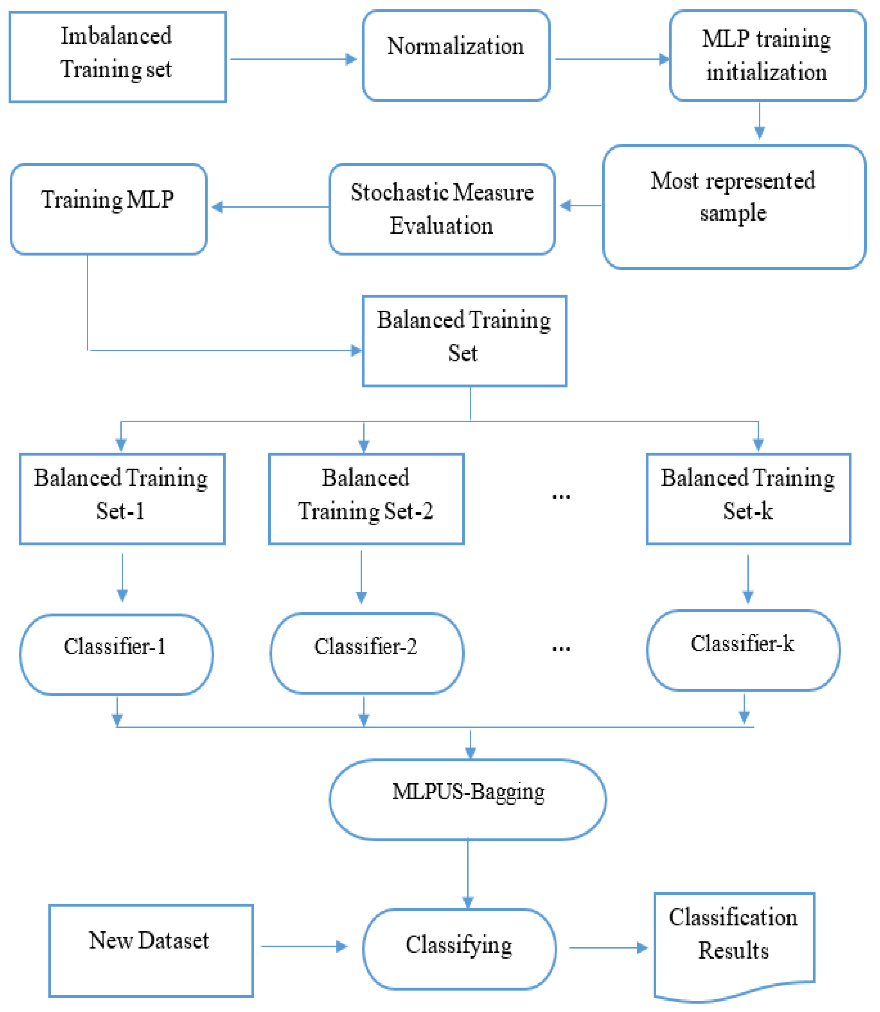
3. Research Materials Proposed Hybrid MLPUS with Bagging Methods
- The sigmoid AF, also called logistic function [39], is defined as follows:
- The AF tanh is the smoother hyperbolic tangent function centered on zero with a range between −1 and 1 [40] and given by:
- The rectified linear unit (ReLU) AF [41] determines the threshold operation on each input element and sets negative values to zero. The formula of ReLU is defined by:
- The Swish AF [42] is defined by
- The exponential linear unit (ELU) AF [43] is given by
- The Exponential linear Squashing (ELiSH) AF [44] is given by:
| Algorithm 1 MultiLayer Perceptron UnderSampling (MLPUS) |
| input Imbalanced Training Set output Balanced Training set
|
| Algorithm 2 Proposed method |
input imbalanced dataset set ; n: Bootstrap size, T: number of iterations, I: Weak Learner
|
4. Experiments
4.1. Datasets
4.1.1. Niger_Rice Dataset Study Area
4.1.2. Niger_Rice Dataset Data Collection
- Precipitation: the cumulative average monthly rainfall (measured in millimeters) in the Niger Office region during the agricultural season (June to November).
- Minimum temperature: the average minimum temperature (in degrees Celsius) in the Niger Office region for the monthly agricultural season (June to November).
- Maximum temperature: the average monthly maximum temperature (in degrees Celsius) in the Niger Office region during the agricultural season (June to November).
- Average temperature: the average monthly average temperature (in degrees Celsius) of the Niger Office region during the agricultural season (June to November).
4.1.3. Niger_Rice Dataset Preprocessing
4.2. Evaluation Metrics and Experimental Setting
4.2.1. Baseline
4.2.2. Performance Evaluation
4.2.3. Experimental Setting
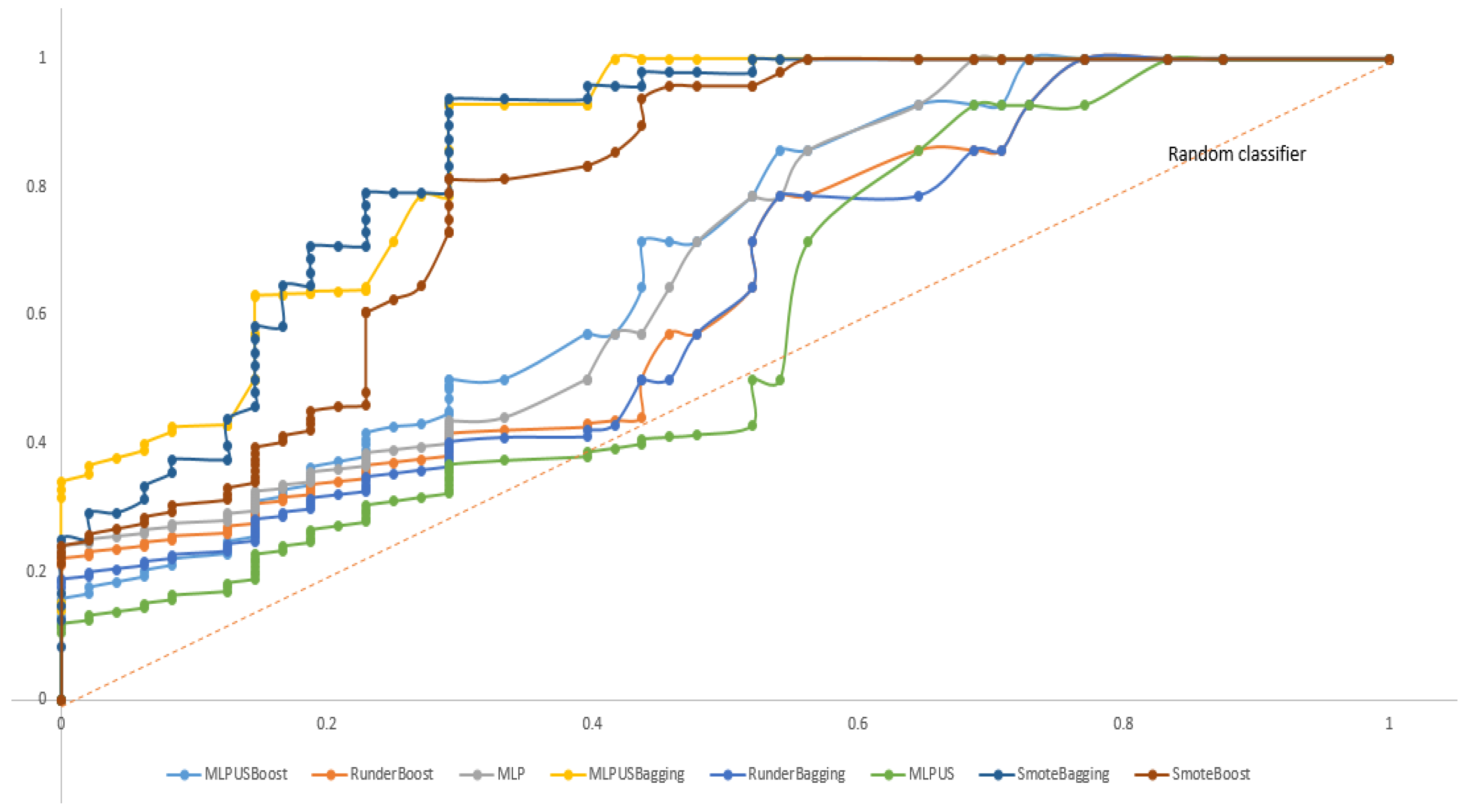
4.3. Experimental Results and Discussion
5. Conclusions
Author Contributions
Funding
Institutional Review Board Statement
Informed Consent Statement
Data Availability Statement
Conflicts of Interest
References
- Zhang, L.; Traore, S.; Ge, J.; Li, Y.; Wang, S.; Zhu, G. Using boosted tree regression and artificial neural networks to forecast upland rice yield under climate change in Sahel. Comput. Electron. Agric. 2019, 166, 105031. [Google Scholar] [CrossRef]
- Zwarts, L.; Beukering, P.; Van Koné, B.; Wymenga, E.; Taylor, D. The Economic and Ecological Effects of Water Management Choices in the Upper Niger River: Development of Decision Support Methods. Int. J. Water Resour. Dev. 2006, 22, 135–156. [Google Scholar] [CrossRef]
- McCoy, J.T.; Auret, L. Machine learning applications in minerals processing: A review. Miner. Eng. 2019, 132, 95–109. [Google Scholar] [CrossRef]
- Prati, R.C.; Batista, G.E.A.P.A.; Silva, D.F. Class imbalance revisited: A new experimental setup to assess the performance of treatment methods. Knowl. Inf. Syst. 2015, 45, 247–270. [Google Scholar] [CrossRef]
- Chawla, N.V.; Japkowicz, N.; Kotcz, A. Editorial. ACM SIGKDD Explor. Newsl. 2004, 6, 1–6. [Google Scholar] [CrossRef]
- Kuncheva, L.I.; Arnaiz-González, Á.; Díez-Pastor, J.-F.; Gunn, I.A.D. Instance selection improves geometric mean accuracy: A study on imbalanced data classification. Prog. Artif. Intell. 2019, 8, 215–228. [Google Scholar] [CrossRef] [Green Version]
- Fan, W.; Stolfo, S.J.; Chan, P.K. AdaCost: Misclassification Cost-sensitive Boosting. Icml 1999, 99, 97–105. [Google Scholar]
- Sun, Y.; Kamel, M.S.; Wong, A.K.C.; Wang, Y. Cost-sensitive boosting for classification of imbalanced data. Pattern Recognit. 2007, 40, 3358–3378. [Google Scholar] [CrossRef]
- Díez-Pastor, J.F.; Rodríguez, J.J.; García-Osorio, C.I.; Kuncheva, L.I. Diversity techniques improve the performance of the best imbalance learning ensembles. Inf. Sci. 2015, 325, 98–117. [Google Scholar] [CrossRef]
- Kaur, H.; Pannu, H.S.; Malhi, A.K. A systematic review on imbalanced data challenges in machine learning: Applications and solutions. ACM Comput. Surv. 2019, 52, 136. [Google Scholar] [CrossRef] [Green Version]
- Barandela, R.; Sánchez, J.S.; Valdovinos, R.M. New Applications of Ensembles of Classifiers. Pattern Anal. Appl. 2003, 6, 245–256. [Google Scholar] [CrossRef]
- Wilson, D.L. Asymptotic Properties of Nearest Neighbor Rules Using Edited Data. IEEE Trans. Syst. Man Cybern. 1972, 2, 408–421. [Google Scholar] [CrossRef] [Green Version]
- Tomek, I. Two modifications of CNN. IEEE Trans. Syst. Man Cybern. 1976, 6, 769–772. [Google Scholar]
- Batista, G.E.A.P.A.; Prati, R.C.; Monard, M.C. A study of the behavior of several methods for balancing machine learning training data. ACM SIGKDD Explor. Newsl. 2004, 6, 20–29. [Google Scholar] [CrossRef]
- Jo, T.; Japkowicz, N. Class imbalances versus small disjuncts. ACM SIGKDD Explor. Newsl. 2004, 6, 40–49. [Google Scholar] [CrossRef]
- Chawla, N.V.; Bowyer, K.W.; Hall, L.O.; Kegelmeyer, W.P. SMOTE: Synthetic minority over-sampling technique. J. Artif. Intell. Res. 2002, 16, 321–357. [Google Scholar] [CrossRef]
- Bunkhumpornpat, C.; Sinapiromsaran, K.; Lursinsap, C. Safe-Level-SMOTE: Safe-Level-Synthetic Minority Over-Sampling TEchnique for Handling the Class Imbalanced Problem. In Pacific-Asia Conference on Knowledge Discovery and Data Mining; Springer: Berlin/Heidelberg, Germany, 2009; pp. 475–482. [Google Scholar]
- Han, H.; Wang, W.-Y.; Mao, B.-H. Borderline-SMOTE: A New Over-Sampling Method in Imbalanced Data Sets Learning. In International Conference on Intelligent Computing; Springer: Berlin/Heidelberg, Germany, 2005; pp. 878–887. [Google Scholar]
- He, H.; Bai, Y.; Garcia, E.A.; Li, S. ADASYN: Adaptive synthetic sampling approach for imbalanced learning. In Proceedings of the 2008 IEEE International Joint Conference on Neural Networks (IEEE World Congress on Computational Intelligence), Hong Kong, China, 1–8 June 2008; pp. 1322–1328. [Google Scholar]
- Kovács, G. Smote-variants: A python implementation of 85 minority oversampling techniques. Neurocomputing 2019, 366, 352–354. [Google Scholar] [CrossRef]
- Xu, Z.; Shen, D.; Nie, T.; Kou, Y. A hybrid sampling algorithm combining M-SMOTE and ENN based on Random forest for medical imbalanced data. J. Biomed. Inform. 2020, 107, 103465. [Google Scholar] [CrossRef]
- Sáez, J.A.; Luengo, J.; Stefanowski, J.; Herrera, F. SMOTE–IPF: Addressing the noisy and borderline examples problem in imbalanced classification by a re-sampling method with filtering. Inf. Sci. 2015, 291, 184–203. [Google Scholar] [CrossRef]
- Zhang, X.; Zhu, C.; Wu, H.; Liu, Z.; Xu, Y. An Imbalance Compensation Framework for Background Subtraction. IEEE Trans. Multimed. 2017, 19, 2425–2438. [Google Scholar] [CrossRef]
- Li, J.; Fong, S.; Wong, R.K.; Chu, V.W. Adaptive multi-objective swarm fusion for imbalanced data classification. Inf. Fusion 2018, 39, 1–24. [Google Scholar] [CrossRef]
- Bailey, J.; Khan, L.; Washio, T.; Dobbie, G.; Huang, J.Z.; Wang, R. Advances in knowledge discovery and data mining: 20th pacific-asia conference, PAKDD 2016 Auckland, New Zealand, April 19–22, 2016 proceedings, part I. Lect. Notes Comput. Sci. 2016, 9651, 14–26. [Google Scholar]
- Kuncheva, L.I. Combining Pattern Classifiers: Methods and Algorithms; John Wiley & Sons: Hoboken, NJ, USA, 2014. [Google Scholar]
- Breiman, L. Bagging predictions. Mach. Learn. 1996, 24, 123–140. [Google Scholar] [CrossRef] [Green Version]
- Freund, Y.; Schapire, R.E.; Hill, M. Experiments with a New Boosting Algorithm. Icml 1996, 96, 148–156. [Google Scholar]
- Wang, S.; Yao, X. Diversity analysis on imbalanced data sets by using ensemble models. In 2009 IEEE Symposium on Computational Intelligence and Data Mining; IEEE: Piscataway, NJ, USA, 2009; pp. 324–331. [Google Scholar]
- Chawla, N.V.; Lazarevic, A.; Hall, L.O.; Bowyer, K.W. SMOTEBoost: Improving Prediction of the Minority Class in Boosting. In European Conference on Principles of Data Mining and Knowledge Discovery; Springer: Berlin/Heidelberg, Germany, 2003; pp. 107–119. [Google Scholar]
- Chen, S.; He, H.; Garcia, E.A. RAMOBoost: Ranked minority oversampling in boosting. IEEE Trans. Neural Netw. 2010, 21, 1624–1642. [Google Scholar] [CrossRef] [PubMed]
- Seiffert, C.; Khoshgoftaar, T.M.; Van Hulse, J.; Napolitano, A. RUSBoost: A hybrid approach to alleviating class imbalance. IEEE Trans. Syst. Man Cybern. Part A Syst. Hum. 2010, 40, 185–197. [Google Scholar] [CrossRef]
- Galar, M.; Fernández, A.; Barrenechea, E.; Herrera, F. EUSBoost: Enhancing ensembles for highly imbalanced data-sets by evolutionary undersampling. Pattern Recognit. 2013, 46, 3460–3471. [Google Scholar] [CrossRef]
- Liu, X.Y.; Wu, J.; Zhou, Z.H. Exploratory undersampling for class-imbalance learning. IEEE Trans. Syst. Man, Cybern. Part B Cybern. 2009, 39, 539–550. [Google Scholar]
- Díez-Pastor, J.F.; Rodríguez, J.J.; García-Osorio, C.; Kuncheva, L.I. Random Balance: Ensembles of variable priors classifiers for imbalanced data. Knowl. Based Syst. 2015, 85, 96–111. [Google Scholar] [CrossRef]
- Galar, M.; Fernandez, A.; Barrenechea, E.; Bustince, H.; Herrera, F. A review on ensembles for the class imbalance problem: Bagging-, boosting-, and hybrid-based approaches. IEEE Trans. Syst. Man Cybern. Part C Appl. Rev. 2012, 42, 463–484. [Google Scholar] [CrossRef]
- Błaszczyński, J.; Deckert, M.; Stefanowski, J.; Wilk, S. Integrating selective pre-processing of imbalanced data with Ivotes ensemble. Lect. Notes Comput. Sci. 2010, 6086, 148–157. [Google Scholar]
- Babar, V.; Ade, R. A Novel Approach for Handling Imbalanced Data in Medical Diagnosis using Undersampling Technique. Commun. Appl. Electron. 2016, 5, 36–42. [Google Scholar] [CrossRef]
- Li, H.; Jiang, X.; Huo, G.; Su, C.; Wang, B. A novel feed rate scheduling method based on Sigmoid function with chord error and kinematics constraints. arXiv 2021, arXiv:2105.05434. [Google Scholar]
- Lecun, Y.; Bengio, Y.; Hinton, G. Deep learning. Nature 2015, 521, 436–444. [Google Scholar] [CrossRef] [PubMed]
- Brown, M.J.; Hutchinson, L.A.; Rainbow, M.J.; Deluzio, K.J.; De Asha, A.R. A comparison of self-selected walking speeds and walking speed variability when data are collected during repeated discrete trials and during continuous walking. J. Appl. Biomech. 2017, 33, 384–387. [Google Scholar] [CrossRef] [PubMed]
- Ramachandran, P.; Zoph, B.; Le Google Brain, Q.V. Searching for activation functions. arXiv 2017, arXiv:1710.05941. [Google Scholar]
- Clevert, D.-A.; Unterthiner, T.; Hochreiter, S. Fast and accurate deep network learning by exponential linear units (elus). arXiv 2015, arXiv:1511.07289. [Google Scholar]
- Basirat, M.; Roth, P.M. The Quest for the Golden Activation Function. arXiv 2018, arXiv:1808.00783. [Google Scholar]
- Ernández, A.F.; Uengo, J.L.; Errac, J.D. KEEL Data-Mining Software Tool: Data Set Repository, Integration of Algorithms and Experimental Analysis Framework. J. Mult. Valued Log. Soft Comput. 2011, 17, 255–287. [Google Scholar]
- Kohonen, T. An introduction to neural computing. Neural Netw. 1988, 1, 3–16. [Google Scholar] [CrossRef]


| Header | Description |
|---|---|
| P | Determines the total amount of precipitation recorded from June to November |
| Max | Represents the average of the maximum temperature recorded from June to November |
| Min | Returns the value of the average of the minimum temperature recorded from June to November |
| Average | Returns the value of the average temperature recorded from June to November |
| Yield | yes or no class (which qualifies the result as good or bad depending on the threshold) |
| No | Dataset’s Name | Att | NI | P | N | IR |
|---|---|---|---|---|---|---|
| 1 | glass1 | 9 | 214 | 76 | 138 | 1.82 |
| 2 | ecoli-0_vs_1 | 7 | 220 | 77 | 143 | 1.86 |
| 3 | wisconsin | 9 | 683 | 239 | 444 | 1.86 |
| 4 | pima | 8 | 768 | 268 | 500 | 1.87 |
| 5 | iris0 | 4 | 150 | 50 | 100 | 2 |
| 6 | glass0 | 9 | 214 | 70 | 144 | 2.06 |
| 7 | yeast1 | 8 | 1484 | 429 | 1055 | 2.46 |
| 8 | haberman | 3 | 306 | 81 | 225 | 2.78 |
| 9 | vehicle2 | 18 | 846 | 218 | 628 | 2.88 |
| 10 | vehicle1 | 18 | 846 | 217 | 629 | 2.9 |
| 11 | vehicle3 | 18 | 846 | 212 | 634 | 2.99 |
| 12 | glass-0-1-2-3_vs_4-5-6 | 9 | 214 | 51 | 163 | 3.2 |
| 13 | vehicle0 | 18 | 846 | 199 | 647 | 3.25 |
| 14 | ecoli1 | 7 | 336 | 77 | 259 | 3.36 |
| 15 | new-thyroid1 | 5 | 215 | 35 | 180 | 5.14 |
| 16 | new-thyroid2 | 5 | 215 | 35 | 180 | 5.14 |
| 17 | ecoli2 | 7 | 336 | 52 | 284 | 5.46 |
| 18 | segment0 | 19 | 2308 | 329 | 1979 | 6.02 |
| 19 | glass6 | 9 | 214 | 29 | 185 | 6.38 |
| 20 | yeast3 | 8 | 1484 | 163 | 1321 | 8.1 |
| 21 | ecoli3 | 7 | 336 | 35 | 301 | 8.6 |
| 22 | page-blocks0 | 10 | 5472 | 559 | 4913 | 8.79 |
| 23 | yeast-2_vs_4 | 8 | 514 | 51 | 463 | 9.08 |
| 24 | yeast-0-5-6-7-9_vs_4 | 8 | 528 | 51 | 477 | 9.35 |
| 25 | vowel0 | 13 | 988 | 90 | 898 | 9.98 |
| 26 | glass-0-1-6_vs_2 | 9 | 192 | 17 | 175 | 10.29 |
| 27 | glass2 | 9 | 214 | 17 | 197 | 11.59 |
| 28 | shuttle-c0-vs-c4 | 9 | 1829 | 123 | 1706 | 13.87 |
| 29 | yeast-1_vs_7 | 7 | 459 | 30 | 429 | 14.3 |
| 30 | glass4 | 9 | 214 | 13 | 201 | 15.47 |
| 31 | ecoli4 | 7 | 336 | 20 | 316 | 15.8 |
| 32 | page-blocks-1-3_vs_4 | 10 | 472 | 28 | 444 | 15.86 |
| 33 | abalone9-18 | 8 | 731 | 42 | 689 | 16.4 |
| 34 | glass-0-1-6_vs_5 | 9 | 184 | 9 | 175 | 19.44 |
| 35 | shuttle-c2-vs-c4 | 9 | 129 | 6 | 123 | 20.5 |
| 36 | yeast-1-4-5-8_vs_7 | 8 | 693 | 30 | 663 | 22.1 |
| 37 | glass5 | 9 | 214 | 9 | 205 | 22.78 |
| 38 | yeast-2_vs_8 | 8 | 482 | 20 | 462 | 23.1 |
| 39 | yeast4 | 8 | 1484 | 51 | 1433 | 28.1 |
| 40 | yeast-1-2-8-9_vs_7 | 8 | 947 | 9 | 938 | 30.57 |
| 41 | yeast5 | 8 | 1484 | 44 | 1440 | 32.73 |
| 42 | ecoli-0-1-3-7_vs_2-6 | 7 | 281 | 7 | 274 | 39.14 |
| 43 | yeast6 | 8 | 1484 | 35 | 1449 | 41.4 |
| 44 | abalone19 | 8 | 4174 | 32 | 4142 | 129.44 |
| 45 | Niger_Rice | 4 | 62 | 14 | 48 | 3.43 |
| Predicted Negative | Predicted Positive | |
|---|---|---|
| Actual Negative | TN | FP |
| Actual Positive | FN | TP |
| Dataset | MLPUS_Bagging | MLP Classifier | MLP Under-Sampling | SMOTE_Bagging | SMOTE_Boost | Under-Bagging | RUS_Boost | MLPUS_Boost |
|---|---|---|---|---|---|---|---|---|
| ecoli-0_vs_1 | 97.91 (2.48) | 99.09 (1.24) | 98.04 (1.79) | 97.92 (1.63) | 97.78 (1.67) | 97.28 (3.32) | 97.14 (2.69) | 97.91 (2.48) |
| ecoli1 | 92.73 (4.60) | 90.17 (2.52) | 92.22 (3.66) | 90.40 (2.83) | 90.16 (2.66) | 93.37 (4.62) | 91.04 (5.06) | 91.82 (6.66) |
| ecoli2 | 97.87 (3.45) | 94.34 (2.88) | 90.33 (4.95) * | 94.54 (2.36) | 94.33 (2.49) | 90.98 (5.62) * | 90.57 (6.44) * | 96.74 (6.26) |
| ecoli3 | 93.43 (6.81) | 93.16 (4.15) | 90.00 (3.91) | 92.50 (2.74) | 93.85 (2.47) | 92.00 (5.18) | 90.00 (5.83) | 92.57 (6.00) |
| glass-0-1-2-3_vs_4-5-6 | 94.73 (6.07) | 90.18 (2.01) * | 95.05 (6.12) | 94.87 (3.11) | 94.64 (3.16) | 94.32 (3.33) | 95.66 (4.16) | 94.52 (5.12) |
| glass0 | 92.00 (5.58) | 80.86 (4.38) * | 71.43 (7.58) * | 86.75 (5.16) * | 88.59 (4.23) * | 77.14 (6.84) * | 76.71 (8.88) * | 92.43 (3.90) |
| glass1 | 77.36 (7.95) | 68.22 (5.40) * | 65.05 (8.34) * | 82.76 (5.20)v | 86.21 (4.53)v | 75.26 (7.42) | 78.82 (5.30) | 74.37 (7.45) |
| glass6 | 88.67 (9.18) | 97.67 (4.03)v | 91.67 (10.21) | 95.72 (2.22)v | 95.79 (2.11)v | 89.33 (8.74) | 88.70 (8.06) | 90.39 (6.99) |
| haberman | 56.87 (7.47) | 74.17 (4.34)v | 62.92 (8.03)v | 71.42 (4.55)v | 69.46 (4.59)v | 62.23 (7.65)v | 64.70 (7.58)v | 59.87 (5.89) |
| iris0 | 98.60 (3.07) | 100.00 (0.00) | 100.00 (0.00) | 99.30 (1.35) | 99.50 (1.02) | 98.60 (2.29) | 99.00 (2.04) | 98.60 (3.07) |
| new-thyroid1 | 94.86 (4.84) | 98.14 (1.95) | 95.71 (3.91) | 97.68 (1.97) | 97.52 (2.18) | 91.71 (6.74) | 93.43 (7.96) | 95.14 (5.35) |
| newthyroid2 | 94.86 (4.84) | 98.14 (1.04) | 100.00 (0.00)v | 98.08 (1.58) | 97.76 (2.03) | 92.57 (6.99) | 94.86 (6.02) | 95.14 (5.35) |
| page-blocks0 | 98.00 (0.85) | 96.69 (0.52) | 93.56 (2.64) * | 97.11 (0.38) | 97.17 (0.42) | 95.31 (1.29) | 94.85 (1.23) | 98.60 (0.96) |
| pima | 77.46 (3.70) | 74.09 (2.75) | 76.49 (3.24) | 78.86 (2.04) | 77.70 (2.23) | 73.76 (4.36) | 71.60 (4.85) * | 73.54 (3.72) |
| segment0 | 97.66 (1.68) | 99.70 (0.33) | 99.08 (1.25) | 99.48 (0.40) | 99.75 (0.28) | 98.24 (0.93) | 98.97 (0.90) | 99.15 (1.01) |
| vehicle0 | 94.57 (2.95) | 96.93 (0.50) | 95.73 (2.11) | 96.40 (1.24) | 97.45 (0.89) | 92.86 (3.07) | 94.57 (2.66) | 95.48 (2.96) |
| vehicle1 | 82.35 (3.13) | 83.21 (2.39) | 77.41 (3.83) * | 81.62 (2.90) | 82.94 (2.27) | 74.83 (5.18) * | 72.39 (4.48) * | 82.49 (3.15) |
| vehicle2 | 75.37 (2.84) | 97.87 (0.89)v | 96.33 (1.88)v | 97.22 (1.07)v | 98.52 (0.83)v | 95.14 (2.80)v | 96.92 (2.07)v | 75.56 (4.71) |
| vehicle3 | 80.43 (4.22) | 82.51 (2.20) | 78.99 (8.92) | 82.16 (2.76) | 82.63 (2.42) | 74.48 (3.70) * | 73.54 (2.65) * | 82.32 (4.23) |
| wisconsin | 99.29 (0.84) | 95.90 (0.85) | 95.39 (2.84) * | 97.16 (0.95) | 97.61 (0.95) | 96.95 (1.38) | 95.86 (1.61) | 99.41 (0.96) |
| yeast1 | 83.91 (1.89) | 77.63 (2.33) * | 69.12 (4.39) * | 78.42 (1.59) * | 76.84 (1.98) * | 71.66 (2.61) * | 69.72 (3.20) * | 81.42 (2.49) |
| yeast3 | 92.21 (3.57) | 94.54 (1.24) | 89.58 (2.69) | 95.06 (1.05) | 94.52 (1.19) | 92.27 (2.23) | 90.49 (2.75) | 91.54 (4.47) |
| abalone19 | 99.23 (0.07) | 73.13 (11.96) * | 86.37 (0.89) * | 98.48 (0.05) | 98.48 (0.05) | 68.85 (7.25) * | 62.69 (9.38) * | 82.56 (11.18) * |
| abalone9-18 | 95.08 (1.01) | 81.87 (10.28) * | 87.50 (2.24) * | 91.72 (1.45) | 90.56 (1.67) * | 72.72 (15.74) * | 65.66 (14.93) * | 84.50 (9.15) * |
| ecoli-0-1-3-7_vs_2-6 | 98.93 (0.97) | 84.67 (22.53) * | 93.58 (1.85) * | 97.57 (0.93) | 98.61 (0.77) | 73.33 (14.91) * | 80.00 (29.81) * | 82.00 (22.53) * |
| ecoli4 | 98.51 (1.49) | 90.50 (9.74) * | 95.92 (1.48) | 97.19 (2.00) | 97.19 (2.23) | 85.00 (16.30) * | 90.00 (10.46) * | 91.00 (8.48) * |
| glass-0-1-6_vs_2 | 89.07 (2.14) | 73.90 (19.18) * | 84.97 (3.20) | 88.52 (3.07) | 83.74 (0.91) | 59.52 (20.48) * | 82.38 (11.86) * | 81.05 (16.34) * |
| glass-0-1-6_vs_5 | 96.73 (1.28) | 84.67 (22.40) * | 97.37 (1.68) | 96.36 (2.99) | 98.46 (2.29) | 93.33 (14.91) | 93.33 (14.91) | 85.67 (17.27) * |
| glass2 | 89.27 (2.59) | 75.33 (21.60) * | 88.02 (2.60) | 87.88 (2.46) | 85.28 (0.95) | 61.90 (12.14) * | 67.62 (11.86) * | 85.90 (14.61) |
| glass4 | 96.72 (2.67) | 93.20 (9.30) | 89.25 (3.51) * | 96.90 (5.80) | 94.26 (3.72) | 80.67 (14.22) * | 88.67 (10.43) * | 92.40 (9.55) |
| glass5 | 97.19 (3.05) | 87.00 (20.14) * | 97.66 (1.53) | 98.18 (2.49) | 98.21 (1.86) | 100.00 (0.00) | 100.00 (0.00) | 92.00 (13.28) |
| page-blocks-1-3_vs_4 | 99.79 (0.47) | 94.33 (9.19) * | 98.31 (0.96) | 99.60 (0.89) | 99.60 (0.89) | 87.73 (9.59) * | 94.70 (4.85) | 98.27 (5.46) |
| shuttle-c0-vs-c4 | 99.95 (0.12) | 99.02 (1.67) | 99.98 (0.05) | 100.00 (0.00) | 100.00 (0.00) | 100.00 (0.00) | 100.00 (0.00) | 99.10 (1.57) |
| shuttle-c2-vs-c4 | 99.23 (1.72) | 68.00 (30.02) * | 98.21 (1.47) | 98.52 (2.03) | 99.26 (1.66) | 90.00 (22.36) * | 90.00 (22.36) * | 92.00 (22.11) * |
| vowel0 | 99.70 (0.28) | 92.22 (3.76) * | 94.19 (1.12) * | 98.14 (0.80) | 98.05 (0.51) | 98.89 (1.52) | 97.78 (2.32) | 94.00 (4.29) |
| yeast-0-5-6-7-9_vs_4 | 91.09 (3.21) | 82.14 (7.22) * | 84.23 (2.09) * | 89.64 (2.45) | 89.12 (1.88) | 85.19 (8.80) * | 81.24 (9.81) * | 86.67 (6.59) * |
| yeast-1-2-8-9_vs_7 | 96.83 (0.37) | 93.33 (8.67) | 97.15 (0.43) | 94.88 (1.02) | 94.17 (0.85) | 70.00 (17.28) * | 61.67 (9.50) * | 96.00 (6.85) |
| yeast-1-4-5-8_vs_7 | 95.67 (0.73) | 94.67 (6.75) | 82.52 (2.03) * | 92.11 (0.80) | 91.70 (0.03) | 53.33 (4.56) * | 61.67 (17.28) * | 97.33 (5.23) |
| yeast-1_vs_7 | 92.59 (2.48) | 90.33 (11.46) | 79.86 (3.18) * | 90.59 (1.97) | 89.16 (1.17) | 73.33 (9.13) * | 75.00 (5.89) * | 98.33 (3.40)v |
| yeast-2_vs_4 | 95.14 (2.05) | 84.65 (9.19) * | 92.55 (1.58) | 94.34 (1.94) | 94.16 (2.39) | 90.10 (10.06) | 89.19 (6.47) * | 89.00 (6.51) * |
| yeast-2_vs_8 | 97.93 (0.74) | 84.50 (9.74) * | 89.91 (2.14) * | 96.21 (1.80) | 96.01 (1.43) | 67.50 (14.25) * | 72.50 (13.69) * | 97.50 (5.10) |
| yeast4 | 97.37 (0.55) | 80.92 (8.44) * | 90.53 (0.90) * | 95.11 (1.28) | 93.62 (2.45) | 73.67 (8.30) * | 69.67 (4.80) * | 85.29 (6.21) * |
| yeast5 | 97.64 (0.89) | 93.67 (6.11) | 99.22 (0.35) | 98.17 (0.75) | 97.97 (0.58) | 97.71 (3.13) | 96.60 (5.01) | 96.59 (5.38) |
| yeast6 | 97.78 (0.77) | 89.71 (10.93) * | 95.78 (0.82) | 97.43 (0.85) | 96.97 (1.34) | 91.43 (7.82) * | 88.57 (8.14) * | 95.43 (6.14) |
| Niger_Rice | 75.60 (16.85) | 72.44 (12.11) | 61.33 (17.26) * | 76.49 (9.45) | 76.21 (8.89) | 60.00 (13.33) * | 58.93 (16.60) * | 72.80 (14.42) |
| (v/-/- *) | (3/22/20) | (3/24/18) | (4/39/2) | (4/38/3) | (2/21/22) | (2/20/23) | (1/34/10) |
| Dataset | MLPUS_Bagging | MLP Classifier | MLP Under-Sampling | SMOTE_Bagging | SMOTE_Boost | Under-Bagging | RUS_Boost | MLPUS_Boost |
|---|---|---|---|---|---|---|---|---|
| ecoli-0_vs_1 | 0.98 (0.02) | 0.99 (0.01) | 0.98 (0.02) | 0.98 (0.02) | 0.98 (0.02) | 0.97 (0.04) | 0.97 (0.03) | 0.98 (0.02) |
| ecoli1 | 0.93 (0.04) | 0.77 (0.07) * | 0.92 (0.04) | 0.87 (0.04) * | 0.87 (0.04) * | 0.94 (0.04) | 0.91 (0.05) | 0.92 (0.06) |
| ecoli2 | 0.98 (0.03) | 0.82 (0.08) * | 0.90 (0.05) * | 0.89 (0.05) * | 0.89 (0.05) * | 0.91 (0.06) * | 0.90 (0.06) * | 0.96 (0.08) |
| ecoli3 | 0.94 (0.06) | 0.68 (0.19) * | 0.90 (0.04) | 0.80 (0.07) * | 0.84 (0.07) * | 0.92 (0.05) | 0.90 (0.06) | 0.93 (0.06) |
| glass-0-1-2-3_vs_4-5-6 | 0.95 (0.06) | 0.78 (0.03) * | 0.95 (0.06) | 0.93 (0.04) | 0.93 (0.04) | 0.94 (0.03) | 0.96 (0.04) | 0.95 (0.05) |
| glass0 | 0.92 (0.05) | 0.72 (0.07) * | 0.71 (0.07) * | 0.87 (0.05) * | 0.89 (0.04) | 0.77 (0.07) * | 0.77 (0.10) * | 0.93 (0.04) |
| glass1 | 0.78 (0.09) | 0.49 (0.09) * | 0.62 (0.12) * | 0.84 (0.05)v | 0.87 (0.04)v | 0.75 (0.07) | 0.79 (0.06) | 0.74 (0.09) |
| glass6 | 0.88 (0.10) | 0.90 (0.17) | 0.91 (0.11) | 0.91 (0.04) | 0.91 (0.05) | 0.90 (0.08) | 0.89 (0.08) | 0.90 (0.07) |
| haberman | 0.51 (0.11) | 0.39 (0.08) * | 0.59 (0.10)v | 0.65 (0.05)v | 0.62 (0.09)v | 0.60 (0.10)v | 0.65 (0.09)v | 0.47 (0.10) |
| iris0 | 0.98 (0.03) | 1.00 (0.00) | 1.00 (0.00) | 0.99 (0.01) | 0.99 (0.01) | 0.99 (0.02) | 0.99 (0.02) | 0.98 (0.03) |
| new-thyroid1 | 0.95 (0.05) | 0.94 (0.06) | 0.96 (0.04) | 0.96 (0.04) | 0.95 (0.04) | 0.92 (0.06) | 0.94 (0.07) | 0.95 (0.05) |
| newthyroid2 | 0.95 (0.05) | 0.94 (0.03) | 1.00 (0.00)v | 0.97 (0.03) | 0.96 (0.04) | 0.93 (0.07) | 0.95 (0.06) | 0.95 (0.05) |
| page-blocks0 | 0.98 (0.01) | 0.83 (0.03) | 0.94 (0.03) | 0.92 (0.01) | 0.92 (0.01) | 0.95 (0.01) | 0.95 (0.01) | 0.99 (0.01) |
| pima | 0.77 (0.04) | 0.62 (0.03) * | 0.77 (0.04) | 0.80 (0.02) | 0.79 (0.02) | 0.74 (0.05) | 0.72 (0.06) | 0.73 (0.04) |
| segment0 | 0.98 (0.02) | 0.99 (0.01) | 0.99 (0.01) | 0.99 (0.01) | 0.99 (0.01) | 0.98 (0.01) | 0.99 (0.01) | 0.99 (0.01) |
| vehicle0 | 0.95 (0.03) | 0.94 (0.01) | 0.96 (0.02) | 0.95 (0.02) | 0.97 (0.01) | 0.93 (0.03) | 0.95 (0.03) | 0.95 (0.03) |
| vehicle1 | 0.83 (0.03) | 0.67 (0.03) * | 0.78 (0.04) * | 0.78 (0.04) * | 0.79 (0.03) | 0.76 (0.05) * | 0.73 (0.05) * | 0.83 (0.03) |
| vehicle2 | 0.75 (0.03) | 0.96 (0.02)v | 0.96 (0.02)v | 0.97 (0.01)v | 0.98 (0.01)v | 0.95 (0.03)v | 0.97 (0.02)v | 0.75 (0.05) |
| vehicle3 | 0.81 (0.04) | 0.64 (0.05) * | 0.80 (0.08) | 0.78 (0.04) | 0.79 (0.03) | 0.75 (0.04) * | 0.74 (0.03) * | 0.83 (0.04) |
| wisconsin | 0.99 (0.01) | 0.94 (0.01) | 0.95 (0.03) | 0.97 (0.01) | 0.98 (0.01) | 0.97 (0.01) | 0.96 (0.02) | 0.99 (0.01) |
| yeast1 | 0.85 (0.02) | 0.56 (0.03) * | 0.70 (0.04) * | 0.76 (0.02) * | 0.74 (0.02) * | 0.72 (0.03) * | 0.69 (0.04) * | 0.82 (0.03) |
| yeast3 | 0.92 (0.04) | 0.75 (0.04) * | 0.90 (0.03) | 0.88 (0.03) * | 0.86 (0.03) * | 0.92 (0.02) | 0.91 (0.03) | 0.92 (0.05) |
| abalone19 | 0.73 (0.14) | 0.00 (0.00) * | 0.87 (0.01)v | 0.00 (0.00) * | 0.00 (0.00) * | 0.71 (0.07) | 0.59 (0.16) * | 0.83 (0.11)v |
| abalone9-18 | 0.82 (0.10) | 0.52 (0.10) * | 0.87 (0.02) | 0.48 (0.10) * | 0.30 (0.26) * | 0.72 (0.16) * | 0.67 (0.12) * | 0.84 (0.09) |
| ecoli-0-1-3-7_vs_2-6 | 0.88 (0.17) | 0.69 (0.41) * | 0.94 (0.02)v | 0.73 (0.09) * | 0.86 (0.08) | 0.60 (0.37) * | 0.73 (0.43) * | 0.86 (0.17) |
| ecoli4 | 0.90 (0.10) | 0.87 (0.13) | 0.96 (0.01) | 0.87 (0.08) | 0.87 (0.10) | 0.88 (0.12) | 0.91 (0.09) | 0.91 (0.09) |
| glass-0-1-6_vs_2 | 0.78 (0.15) | 0.07 (0.15) * | 0.86 (0.03)v | 0.52 (0.10) * | 0.00 (0.00) * | 0.54 (0.25) * | 0.81 (0.14) | 0.84 (0.14)v |
| glass-0-1-6_vs_5 | 0.80 (0.33) | 0.59 (0.33) * | 0.97 (0.02)v | 0.78 (0.23) | 0.93 (0.11)v | 0.93 (0.15)v | 0.93 (0.15)v | 0.85 (0.22) |
| glass2 | 0.81 (0.16) | 0.08 (0.18) * | 0.89 (0.02)v | 0.34 (0.22) * | 0.00 (0.00) * | 0.66 (0.12) * | 0.65 (0.17) * | 0.88 (0.12)v |
| glass4 | 0.93 (0.10) | 0.75 (0.21) * | 0.89 (0.04) | 0.88 (0.22) | 0.68 (0.21) * | 0.82 (0.12) * | 0.89 (0.10) | 0.92 (0.11) |
| glass5 | 0.84 (0.29) | 0.65 (0.41) * | 0.98 (0.02)v | 0.87 (0.18) | 0.88 (0.14) | 1.00 (0.00)v | 1.00 (0.00)v | 0.91 (0.15)v |
| page-blocks-1-3_vs_4 | 0.94 (0.10) | 0.98 (0.03) | 0.98 (0.01) | 0.98 (0.04) | 0.98 (0.04) | 0.89 (0.09) | 0.95 (0.05) | 0.98 (0.06) |
| shuttle-c0-vs-c4 | 0.99 (0.02) | 1.00 (0.01) | 1.00 (0.00) | 1.00 (0.00) | 1.00 (0.00) | 1.00 (0.00) | 1.00 (0.00) | 0.99 (0.02) |
| shuttle-c2-vs-c4 | 0.63 (0.40) | 0.80 (0.45)v | 0.98 (0.01)v | 0.87 (0.18)v | 0.93 (0.15)v | 0.80 (0.45)v | 0.80 (0.45)v | 0.90 (0.29)v |
| vowel0 | 0.92 (0.04) | 0.98 (0.02)v | 0.94 (0.01) | 0.95 (0.02) | 0.94 (0.02) | 0.99 (0.02)v | 0.98 (0.02)v | 0.94 (0.04) |
| yeast-0-5-6-7-9_vs_4 | 0.82 (0.09) | 0.46 (0.20) * | 0.85 (0.02) | 0.67 (0.09) * | 0.66 (0.08) * | 0.82 (0.14) | 0.77 (0.18) * | 0.86 (0.07) |
| yeast-1-2-8-9_vs_7 | 0.94 (0.07) | 0.16 (0.14) * | 0.19 (0.18) * | 0.34 (0.19) * | 0.26 (0.07) * | 0.65 (0.26) * | 0.58 (0.19) * | 0.97 (0.06) |
| yeast-1-4-5-8_vs_7 | 0.95 (0.06) | 0.19 (0.17) * | 0.84 (0.02) * | 0.12 (0.12) * | 0.03 (0.06) * | 0.57 (0.09) * | 0.57 (0.19) * | 0.98 (0.05) |
| yeast-1_vs_7 | 0.92 (0.09) | 0.30 (0.19) * | 0.80 (0.03) * | 0.45 (0.16) * | 0.35 (0.11) * | 0.68 (0.22) * | 0.74 (0.07) * | 0.98 (0.03) |
| yeast-2_vs_4 | 0.85 (0.09) | 0.73 (0.13) * | 0.93 (0.02)v | 0.84 (0.06) | 0.83 (0.08) | 0.89 (0.13) | 0.89 (0.07) | 0.89 (0.07) |
| yeast-2_vs_8 | 0.82 (0.13) | 0.69 (0.10) * | 0.89 (0.03)v | 0.68 (0.17) * | 0.67 (0.14) * | 0.65 (0.18) * | 0.71 (0.11) * | 0.98 (0.05) |
| yeast4 | 0.80 (0.10) | 0.48 (0.14) * | 0.91 (0.01)v | 0.52 (0.11) * | 0.51 (0.11) * | 0.74 (0.10) * | 0.67 (0.09) * | 0.85 (0.08) |
| yeast5 | 0.94 (0.06) | 0.63 (0.11) * | 0.99 (0.00) | 0.85 (0.06) * | 0.83 (0.04) * | 0.98 (0.03) | 0.97 (0.05) | 0.97 (0.06) |
| yeast6 | 0.88 (0.14) | 0.47 (0.22) * | 0.96 (0.01)v | 0.68 (0.11) * | 0.64 (0.17) * | 0.91 (0.08)v | 0.88 (0.09) | 0.96 (0.06)v |
| Niger_Rice | 0.73 (0.19) | 0.82 (0.08)v | 0.57 (0.20) * | 0.76 (0.08) | 0.76 (0.08) | 0.55 (0.21) * | 0.54 (0.23) * | 0. 69 (0.17) * |
| (v/-/- *) | (4/13/28) | (14/22/9) | (4/21/20) | (5/22/18) | (7/22/16) | (6/23/16) | (6/38/1) |
| Dataset | MLPUS_Bagging | MLP Classifier | MLP Under-Sampling | SMOTE_Bagging | SMOTE_Boost | Under-Bagging | RUS_Boost | MLPUS_Boost |
|---|---|---|---|---|---|---|---|---|
| ecoli-0_vs_1 | 0.98 (0.04) | 0.98 (0.00) | 0.98 (0.03) | 0.97 (0.02) | 0.98 (0.02) | 0.97 (0.05) | 0.97 (0.04) | 0.97 (0.04) |
| ecoli1 | 0.93 (0.06) | 0.84 (0.04) * | 0.92 (0.07) | 0.90 (0.04) | 0.90 (0.04) | 0.93 (0.06) | 0.91 (0.07) | 0.92 (0.08) |
| ecoli2 | 0.98 (0.05) | 0.90 (0.06) * | 0.90 (0.07) * | 0.92 (0.04) * | 0.92 (0.04) * | 0.91 (0.09) * | 0.90 (0.09) * | 0.96 (0.07) |
| ecoli3 | 0.93 (0.08) | 0.83 (0.10) * | 0.90 (0.07) | 0.87 (0.05) * | 0.90 (0.04) | 0.92 (0.08) | 0.90 (0.10) | 0.92 (0.10) |
| glass-0-1-2-3_vs_4-5-6 | 0.94 (0.08) | 0.83 (0.04) * | 0.95 (0.07) | 0.94 (0.05) | 0.94 (0.05) | 0.94 (0.06) | 0.96 (0.06) | 0.94 (0.07) |
| glass0 | 0.92 (0.08) | 0.79 (0.05) * | 0.71 (0.13) * | 0.87 (0.07) * | 0.88 (0.06) | 0.77 (0.10) * | 0.76 (0.14) * | 0.92 (0.07) |
| glass1 | 0.77 (0.12) | 0.60 (0.11) * | 0.65 (0.09) * | 0.82 (0.07) | 0.86 (0.06)v | 0.75 (0.09) | 0.79 (0.10) | 0.74 (0.12) |
| glass6 | 0.88 (0.14) | 0.93 (0.05)v | 0.92 (0.10)v | 0.95 (0.05)v | 0.94 (0.04)v | 0.89 (0.11) | 0.89 (0.10) | 0.90 (0.13) |
| haberman | 0.56 (0.14) | 0.53 (0.06) | 0.62 (0.09)v | 0.70 (0.07)v | 0.68 (0.09)v | 0.62 (0.11)v | 0.65 (0.11)v | 0.56 (0.19) |
| iris0 | 0.98 (0.00) | 1.00 (0.00) | 1.00 (0.00) | 0.99 (0.00) | 0.99 (0.00) | 0.98 (0.00) | 0.99 (0.00) | 0.98 (0.00) |
| new-thyroid1 | 0.95 (0.07) | 0.96 (0.04) | 0.95 (0.07) | 0.96 (0.03) | 0.97 (0.04) | 0.91 (0.10) | 0.93 (0.10) | 0.95 (0.07) |
| newthyroid2 | 0.95 (0.07) | 0.96 (0.04) | 1.00 (0.00)v | 0.98 (0.03) | 0.97 (0.04) | 0.92 (0.09) | 0.94 (0.07) | 0.95 (0.07) |
| page-blocks0 | 0.98 (0.01) | 0.88 (0.00) * | 0.93 (0.03) * | 0.95 (0.00) | 0.95 (0.00) | 0.95 (0.02) | 0.95 (0.02) | 0.99 (0.01) |
| pima | 0.77 (0.05) | 0.70 (0.07) | 0.76 (0.05) | 0.79 (0.03) | 0.78 (0.03) | 0.73 (0.06) | 0.71 (0.07) | 0.73 (0.06) |
| segment0 | 0.98 (0.02) | 0.99 (0.00) | 0.99 (0.01) | 0.99 (0.00) | 0.99 (0.00) | 0.98 (0.01) | 0.99 (0.01) | 0.99 (0.01) |
| vehicle0 | 0.94 (0.04) | 0.96 (0.01) | 0.95 (0.03) | 0.96 (0.02) | 0.97 (0.01) | 0.93 (0.04) | 0.94 (0.03) | 0.95 (0.04) |
| vehicle1 | 0.82 (0.05) | 0.77 (0.04) * | 0.77 (0.05) * | 0.81 (0.05) | 0.82 (0.04) | 0.75 (0.07) * | 0.72 (0.06) * | 0.82 (0.05) |
| vehicle2 | 0.75 (0.06) | 0.97 (0.02)v | 0.96 (0.03)v | 0.97 (0.01)v | 0.98 (0.01)v | 0.95 (0.03)v | 0.96 (0.03)v | 0.75 (0.07) |
| vehicle3 | 0.80 (0.07) | 0.74 (0.05) * | 0.79 (0.08) | 0.81 (0.04) | 0.82 (0.04) | 0.74 (0.06) * | 0.73 (0.06) * | 0.82 (0.06) |
| wisconsin | 0.99 (0.01) | 0.96 (0.02) | 0.95 (0.04) | 0.97 (0.01) | 0.97 (0.01) | 0.97 (0.02) | 0.95 (0.03) | 0.99 (0.01) |
| yeast1 | 0.83 (0.03) | 0.66 (0.02) * | 0.69 (0.05) * | 0.78 (0.03) * | 0.76 (0.03) * | 0.71 (0.04) * | 0.69 (0.06) * | 0.81 (0.03) |
| yeast3 | 0.92 (0.06) | 0.85 (0.04) * | 0.89 (0.03) * | 0.92 (0.02) | 0.91 (0.02) | 0.92 (0.04) | 0.90 (0.05) | 0.91 (0.07) |
| abalone19 | 0.73 (0.19) | 0.00 (0.00) * | 0.86 (0.01)v | 0.00 (0.00) * | 0.00 (0.00) * | 0.68 (0.19) * | 0.63 (0.20) * | 0.83 (0.16)v |
| abalone9-18 | 0.82 (0.15) | 0.68 (0.03) * | 0.87 (0.02) | 0.60 (0.03) * | 0.49 (0.07) * | 0.72 (0.16) * | 0.65 (0.20) * | 0.84 (0.14) |
| ecoli-0-1-3-7_vs_2-6 | 0.83 (0.21) | 0.84 (0.07) | 0.93 (0.03)v | 0.83 (0.04) | 0.93 (0.04)v | 0.73 (0.30) * | 0.85 (0.31) | 0.80 (0.25) |
| ecoli4 | 0.90 (0.15) | 0.92 (0.04) | 0.96 (0.02)v | 0.92 (0.03) | 0.92 (0.04) | 0.84 (0.20) * | 0.90 (0.16) | 0.91 (0.14) |
| glass-0-1-6_vs_2 | 0.73 (0.22) | 0.22 (0.05) * | 0.85 (0.05)v | 0.61 (0.05) * | 0.00 (0.00) * | 0.60 (0.30) * | 0.83 (0.19)v | 0.80 (0.19)v |
| glass-0-1-6_vs_5 | 0.85 (0.28) | 0.77 (0.09) * | 0.97 (0.02)v | 0.90 (0.05) | 0.97 (0.05)v | 0.95 (0.00)v | 0.95 (0.00)v | 0.86 (0.25) |
| glass2 | 0.73 (0.18) | 0.26 (0.04) * | 0.88 (0.05)v | 0.49 (0.04) * | 0.00 (0.00) * | 0.60 (0.22) * | 0.67 (0.17) * | 0.85 (0.16)v |
| glass4 | 0.94 (0.13) | 0.90 (0.08) * | 0.89 (0.05) * | 0.94 (0.08) | 0.77 (0.07) * | 0.81 (0.16) * | 0.90 (0.16) | 0.93 (0.14) |
| glass5 | 0.88 (0.25) | 0.83 (0.12) * | 0.97 (0.03)v | 0.93 (0.04) | 0.94 (0.05)v | 1.00 (0.00)v | 1.00 (0.00)v | 0.93 (0.18) |
| page-blocks-1-3_vs_4 | 0.94 (0.11) | 1.00 (0.00)v | 0.98 (0.01) | 1.00 (0.00)v | 0.99 (0.02) | 0.88 (0.10) | 0.94 (0.00) | 0.98 (0.06) |
| shuttle-c0-vs-c4 | 0.99 (0.02) | 0.99 (0.00) | 1.00 (0.00) | 1.00 (0.00) | 1.00 (0.00) | 1.00 (0.00) | 1.00 (0.00) | 0.99 (0.02) |
| shuttle-c2-vs-c4 | 0.71 (0.44) | 0.89 (0.00)v | 0.98 (0.02)v | 0.89 (0.00)v | 0.95 (0.00)v | 0.89 (0.00)v | 0.89 (0.00)v | 0.94 (0.24)v |
| vowel0 | 0.92 (0.05) | 0.99 (0.00)v | 0.94 (0.02) | 0.97 (0.02) | 0.96 (0.03) | 0.99 (0.02)v | 0.98 (0.03)v | 0.94 (0.05) |
| yeast-0-5-6-7-9_vs_4 | 0.82 (0.13) | 0.63 (0.06) * | 0.84 (0.03) | 0.77 (0.03) | 0.77 (0.05) | 0.85 (0.14) | 0.80 (0.19) | 0.86 (0.1) |
| yeast-1-2-8-9_vs_7 | 0.93 (0.07) | 0.32 (0.00) * | 0.33 (0.00) * | 0.48 (0.04) * | 0.41 (0.02) * | 0.70 (0.25) * | 0.61 (0.27) * | 0.96 (0.00) |
| yeast-1-4-5-8_vs_7 | 0.94 (0.06) | 0.36 (0.04) * | 0.82 (0.03) * | 0.26 (0.00) * | 0.14 (0.00) * | 0.52 (0.18) * | 0.61 (0.22) * | 0.97 (0.00) |
| yeast-1_vs_7 | 0.90 (0.00) | 0.51 (0.08) * | 0.80 (0.04) * | 0.57 (0.04) * | 0.49 (0.03) * | 0.73 (0.2) * | 0.75 (0.15) * | 0.98 (0.00)v |
| yeast-2_vs_4 | 0.85 (0.12) | 0.82 (0.04) | 0.92 (0.02)v | 0.90 (0.05) | 0.89 (0.05) | 0.90 (0.17) | 0.89 (0.10) | 0.89 (0.09) |
| yeast-2_vs_8 | 0.84 (0.15) | 0.74 (0.00) * | 0.90 (0.03) | 0.74 (0.00) * | 0.73 (0.00) * | 0.67 (0.31) * | 0.72 (0.26) * | 0.97 (0.00)v |
| yeast4 | 0.81 (0.14) | 0.61 (0.00) * | 0.90 (0.01)v | 0.63 (0.03) * | 0.68 (0.04) * | 0.74 (0.15) * | 0.70 (0.16) * | 0.85 (0.12) |
| yeast5 | 0.93 (0.09) | 0.81 (0.04) * | 0.99 (0.00)v | 0.93 (0.03) | 0.91 (0.03) | 0.97 (0.00) | 0.96 (0.05) | 0.96 (0.06) |
| yeast6 | 0.90 (0.14) | 0.67 (0.05) * | 0.96 (0.01) | 0.78 (0.00) * | 0.76 (0.04) * | 0.91 (0.10) | 0.88 (0.10) | 0.95 (0.09) |
| Niger_Rice | 0.76 (0.24) | 0.59 (0.18) * | 0.60 (0.26) | 0.77 (0.14) | 0.76 (0.15) | 0.60 (0.29) * | 0.60 (0.34) * | 0.73 (0.22) |
| (v/-/-*) | (5/13/27) | (14/20/11) | (5/26/14) | (8/24/13) | (6/21/18) | (7/24/14) | (6/39/0) |
| Dataset | MLPUS_Bagging | MLP Classifier | MLP Under-Sampling | SMOTE_Bagging | SMOTE_Boost | Under-Bagging | RUS_Boost | MLPUS_Boost |
|---|---|---|---|---|---|---|---|---|
| ecoli-0_vs_1 | 0.99 (0.02) | 1.00 (0.01) | 1.00 (0.00) | 0.99 (0.01) | 0.99 (0.01) | 0.99 (0.02) | 0.99 (0.02) | 0.99 (0.02) |
| ecoli1 | 0.98 (0.03) | 0.96 (0.02) | 0.97 (0.02) | 0.96 (0.02) | 0.96 (0.02) | 0.95 (0.04) | 0.95 (0.04) | 0.95 (0.07) |
| ecoli2 | 0.99 (0.03) | 0.96 (0.03) | 0.95 (0.06) | 0.97 (0.02) | 0.98 ( 0.02) | 0.94 (0.05) * | 0.95 (0.06) * | 0.97 (0.05) |
| ecoli3 | 0.99 (0.01) | 0.90 (0.09) * | 0.93 (0.07) * | 0.96 (0.02) | 0.97 (0.02) | 0.92 (0.07) * | 0.92 (0.07) * | 0.94 (0.05) * |
| glass-0-1-2-3_vs_4-5-6 | 0.98 (0.02) | 0.95 (0.04) | 0.96 (0.08) | 0.98 (0.02) | 0.99 (0.01) | 0.98 (0.03) | 0.97 (0.04) | 0.95 (0.05) |
| glass0 | 0.96 (0.04) | 0.84 (0.05) * | 0.79 (0.05) * | 0.94 (0.03) | 0.95 (0.02) | 0.86 (0.07) * | 0.86 (0.07) * | 0.97 (0.03) |
| glass1 | 0.85 (0.08) | 0.71 (0.03) * | 0.68 (0.04) * | 0.90 (0.04)v | 0.93 (0.03)v | 0.84 (0.06) | 0.86 (0.06) | 0.83 (0.08) |
| glass6 | 0.97 (0.05) | 0.95 (0.07) | 0.91 (0.16) * | 0.96 (0.04) | 0.98 (0.02) | 0.94 (0.06) | 0.91 (0.08) * | 0.96 (0.06) |
| haberman | 0.64 (0.10) | 0.68 (0.08) | 0.63 (0.11) | 0.78 (0.04)v | 0.70 (0.04) | 0.63 (0.08) | 0.65 (0.08) | 0.61 (0.05) |
| iris0 | 1.00 (0.00) | 1.00 (0.00) | 1.00 (0.00) | 0.99 (0.01) | 0.99 (0.01) | 0.99 (0.02) | 0.99 (0.02) | 0.99 (0.03) |
| new-thyroid1 | 0.99 (0.03) | 1.00 (0.00) | 0.99 (0.02) | 1.00 (0.01) | 0.98 (0.03) | 0.98 (0.03) | 0.96 (0.07) | 0.98 (0.04) |
| newthyroid2 | 0.99 (0.03) | 1.00 (0.00) | 1.00 (0.00) | 1.00 (0.00) | 0.99 (0.02) | 0.99 (0.02) | 0.97 (0.05) | 0.98 (0.04) |
| page-blocks0 | 1.00 (0.00) | 0.97 (0.02) | 0.98 (0.02) | 0.99 (0.00) | 0.99 (0.00) | 0.99 (0.01) | 0.98 (0.01) | 1.00 (0.00) |
| pima | 0.84 (0.03) | 0.82 (0.04) | 0.84 (0.03) | 0.86 (0.02) | 0.85 (0.02) | 0.80 (0.05) | 0.78 (0.04) * | 0.81 (0.03) |
| segment0 | 1.00 (0.01) | 1.00 (0.00) | 1.00 (0.00) | 1.00 (0.00) | 1.00 (0.00) | 1.00 (0.00) | 0.99 (0.01) | 1.00 (0.01) |
| vehicle0 | 0.99 (0.02) | 0.99 (0.01) | 0.99 (0.01) | 0.99 (0.00) | 1.00 (0.00) | 0.98 (0.02) | 0.99 (0.01) | 0.99 (0.03) |
| vehicle1 | 0.91 (0.03) | 0.90 (0.02) | 0.85 (0.05) * | 0.90 (0.02) | 0.91 (0.02) | 0.82 (0.04) * | 0.79 (0.05) * | 0.90 (0.03) |
| vehicle2 | 0.84 (0.03) | 0.99 (0.02)v | 0.98 (0.02)v | 0.99 (0.00)v | 1.00 (0.00)v | 0.98 (0.02)v | 0.99 (0.01)v | 0.84 (0.04) |
| vehicle3 | 0.89 (0.04) | 0.87 (0.03) | 0.86 (0.07) | 0.91 (0.02) | 0.91 (0.02) | 0.83 (0.03) * | 0.83 (0.04) * | 0.90 (0.03) |
| wisconsin | 1.00 (0.00) | 0.99 (0.00) | 0.99 (0.01) | 0.99 (0.01) | 0.99 (0.01) | 0.99 (0.01) | 0.99 (0.01) | 1.00 (0.01) |
| yeast1 | 0.91 (0.02) | 0.79 (0.03) * | 0.79 (0.04) * | 0.86 (0.02) * | 0.85 (0.02) * | 0.79 (0.02) * | 0.76 (0.03) * | 0.90 (0.02) |
| yeast3 | 0.97 (0.02) | 0.97 (0.01) | 0.96 (0.01) | 0.98 (0.01) | 0.97 (0.01) | 0.97 (0.02) | 0.96 (0.02) | 0.98 (0.02) |
| abalone19 | 0.82 (0.16) | 0.83 (0.03) | 0.94 (0.01)v | 0.86 (0.05) | 0.77 (0.05) * | 0.77 (0.10) * | 0.70 (0.11) * | 0.90 (0.13)v |
| abalone9-18 | 0.90 (0.09) | 0.92 (0.04) | 0.94 (0.01) | 0.88 (0.03) | 0.83 (0.05) * | 0.79 (0.17) * | 0.74 (0.19) * | 0.94 (0.07) |
| ecoli-0-1-3-7_vs_2-6 | 0.89 (0.24) | 0.94 (0.12) | 0.99 (0.01)v | 0.93 (0.09) | 0.98 (0.04)v | 1.00 (0.00)v | 0.85 (0.22) | 0.88 (0.23) |
| ecoli4 | 0.98 (0.05) | 0.99 (0.01) | 0.99 (0.01) | 0.98 (0.03) | 0.99 (0.01) | 0.95 (0.11) | 1.00 (0.00) | 0.98 (0.06) |
| glass-0-1-6_vs_2 | 0.89 (0.15) | 0.81 (0.14) * | 0.88 (0.04) | 0.87 (0.10) | 0.80 (0.08) * | 0.78 (0.25) * | 0.87 (0.16) | 0.90 (0.15) |
| glass-0-1-6_vs_5 | 0.94 (0.15) | 0.95 (0.06) | 1.00 (0.01) | 0.98 (0.01) | 1.00 (0.01) | 0.95 (0.11) | 0.95 (0.11) | 0.87 (0.18) * |
| glass2 | 0.90 (0.12) | 0.74 (0.13) * | 0.90 (0.03) | 0.91 (0.05) | 0.83 (0.04) * | 0.74 (0.26) * | 0.75 (0.17) * | 0.91 (0.13) |
| glass4 | 0.99 (0.03) | 0.98 (0.02) | 0.97 (0.02) | 0.95 (0.11) | 0.91 (0.19) * | 0.88 (0.11) * | 0.84 (0.15) * | 0.93 (0.09) |
| glass5 | 0.95 (0.12) | 0.89 (0.21) * | 1.00 (0.01) | 1.00 (0.01) | 1.00 (0.00) | 1.00 (0.00) | 1.00 (0.00) | 0.93 (0.11) |
| page-blocks-1-3_vs_4 | 0.99 (0.05) | 1.00 (0.00) | 1.00 (0.00) | 1.00 (0.00) | 1.00 (0.00) | 0.96 (0.04) | 1.00 (0.01) | 0.99 (0.03) |
| shuttle-c0-vs-c4 | 1.00 (0.01) | 0.99 (0.02) | 1.00 (0.00) | 1.00 (0.00) | 1.00 (0.00) | 1.00 (0.00) | 1.00 (0.00) | 0.99 (0.02) |
| shuttle-c2-vs-c4 | 0.89 (0.24) | 1.00 (0.00)v | 1.00 (0.01)v | 0.95 (0.11)v | 0.95 (0.11) | 0.90 (0.22) | 0.90 (0.22) | 0.94 (0.17) |
| vowel0 | 0.96 (0.03) | 1.00 (0.00) | 0.98 (0.00) | 1.00 (0.01) | 1.00 (0.00) | 1.00 (0.00) | 1.00 (0.00) | 0.98 (0.03) |
| yeast-0-5-6-7-9_vs_4 | 0.91 (0.04) | 0.82 (0.10) * | 0.93 (0.02) | 0.91 (0.05) | 0.90 (0.05) | 0.89 (0.07) | 0.92 (0.03) | 0.95 (0.04) |
| yeast-1-2-8-9_vs_7 | 0.99 (0.03) | 0.70 (0.10) * | 0.80 (0.07) * | 0.86 (0.06) * | 0.82 (0.02) * | 0.72 (0.19) * | 0.70 (0.12) * | 0.98 (0.06) |
| yeast-1-4-5-8_vs_7 | 0.99 (0.03) | 0.70 (0.14) * | 0.88 (0.02) * | 0.83 (0.04) * | 0.78 (0.07) * | 0.66 (0.05) * | 0.63 (0.13) * | 0.97 (0.05) |
| yeast-1_vs_7 | 0.98 (0.03) | 0.81 (0.07) * | 0.87 (0.02) * | 0.91 (0.05) * | 0.86 (0.05) * | 0.84 (0.07) * | 0.84 (0.09) * | 0.98 (0.04) |
| yeast-2_vs_4 | 0.95 (0.04) | 0.94 (0.06) | 0.98 (0.01) | 0.98 (0.02) | 0.98 (0.01) | 0.96 (0.06) | 0.97 (0.03) | 0.97 (0.02) |
| yeast-2_vs_8 | 0.92 (0.12) | 0.85 (0.14) * | 0.93 (0.02) | 0.92 (0.07) | 0.91 (0.06) | 0.76 (0.17) * | 0.73 (0.19) * | 0.99 (0.03) |
| yeast4 | 0.91 (0.07) | 0.88 (0.05) | 0.97 (0.00)v | 0.96 (0.02) | 0.93 (0.02) | 0.86 (0.10) | 0.81 (0.05) * | 0.95 (0.03) |
| yeast5 | 0.99 (0.02) | 0.98 (0.03) | 1.00 (0.00) | 0.99 (0.01) | 0.99 (0.00) | 0.99 (0.03) | 0.97 (0.05) | 0.99 (0.02) |
| yeast6 | 0.97 (0.05) | 0.95 (0.04) | 0.99 (0.00) | 0.92 (0.08) | 0.95 (0.02) | 0.90 (0.07) | 0.90 (0.12) | 1.00 (0.01) |
| Niger_Rice | 0.86 (0.17) | 0.76 (0.21) * | 0.64 (0.26) * | 0.87 (0.08) | 0.84 (0.08) | 0.72 (0.19) * | 0.75 (0.21) * | 0.80 (0.18) * |
| (v/-/- *) | (2/30/13) | (5/30/10) | (4/37/4) | (3/33/9) | (2/27/16) | (1/26/18) | (1/41/3) |
Publisher’s Note: MDPI stays neutral with regard to jurisdictional claims in published maps and institutional affiliations. |
© 2021 by the authors. Licensee MDPI, Basel, Switzerland. This article is an open access article distributed under the terms and conditions of the Creative Commons Attribution (CC BY) license (https://creativecommons.org/licenses/by/4.0/).
Share and Cite
Diallo, M.; Xiong, S.; Emiru, E.D.; Fesseha, A.; Abdulsalami, A.O.; Elaziz, M.A. A Hybrid MultiLayer Perceptron Under-Sampling with Bagging Dealing with a Real-Life Imbalanced Rice Dataset. Information 2021, 12, 291. https://0-doi-org.brum.beds.ac.uk/10.3390/info12080291
Diallo M, Xiong S, Emiru ED, Fesseha A, Abdulsalami AO, Elaziz MA. A Hybrid MultiLayer Perceptron Under-Sampling with Bagging Dealing with a Real-Life Imbalanced Rice Dataset. Information. 2021; 12(8):291. https://0-doi-org.brum.beds.ac.uk/10.3390/info12080291
Chicago/Turabian StyleDiallo, Moussa, Shengwu Xiong, Eshete Derb Emiru, Awet Fesseha, Aminu Onimisi Abdulsalami, and Mohamed Abd Elaziz. 2021. "A Hybrid MultiLayer Perceptron Under-Sampling with Bagging Dealing with a Real-Life Imbalanced Rice Dataset" Information 12, no. 8: 291. https://0-doi-org.brum.beds.ac.uk/10.3390/info12080291