
Semantic Systematicity in Connectionist Language Production †


1
Department of Language Science and Technology, Saarland University, 66123 Saarbrücken, Germany
2
Applied Cognitive Science Lab, The Pennsylvania State University, State College, PA 16802, USA
*
Author to whom correspondence should be addressed.
†
This paper is an extended version of our paper published in Calvillo, J., Brouwer, H., and Crocker, M.W. Connectionist Semantic Systematicity in Language Production. In Proceedings of the 38th Annual Conference of the Cognitive Science Society, Austin, TX, USA, 10–13 August 2016.
Information 2021, 12(8), 329; https://0-doi-org.brum.beds.ac.uk/10.3390/info12080329
Submission received: 14 July 2021
/
Revised: 6 August 2021
/
Accepted: 10 August 2021
/
Published: 16 August 2021
(This article belongs to the Special Issue Neural Natural Language Generation)
Abstract
:Decades of studies trying to define the extent to which artificial neural networks can exhibit systematicity suggest that systematicity can be achieved by connectionist models but not by default. Here we present a novel connectionist model of sentence production that employs rich situation model representations originally proposed for modeling systematicity in comprehension. The high performance of our model demonstrates that such representations are also well suited to model language production. Furthermore, the model can produce multiple novel sentences for previously unseen situations, including in a different voice (actives vs. passive) and with words in new syntactic roles, thus demonstrating semantic and syntactic generalization and arguably systematicity. Our results provide yet further evidence that such connectionist approaches can achieve systematicity, in production as well as comprehension. We propose our positive results to be a consequence of the regularities of the microworld from which the semantic representations are derived, which provides a sufficient structure from which the neural network can interpret novel inputs.
1. Introduction
During language comprehension, utterances are mapped to their meaning and vice versa during language production. An important challenge is that the number of utterances of a language, and meanings that can be represented, is infinite. Consequently, we cannot memorize all possible utterances/meanings. From a finite set of utterances to which we are exposed during language acquisition, we can generalize and produce/comprehend an infinite number of utterances [1].
Systematicity refers to this ability to generalize from known instances to novel ones, profiting from the regularities between them, in a manner similar to how (rule-based) symbolic functions operate over variables, processing uniformly or systematically the variables of the same type. This has been proposed to be ubiquitous in human cognition, and it is even a law of cognitive systems [2,3]. Other ways to refer to this notion are “compositionality” and “compositional generalization”.
Fodor and Pylyshyn [2] started a debate arguing that connectionist cognitive models (i.e., models implementing artificial neural networks) cannot behave systematically, and even if they could, they would need to implement a symbol system, similar to the one proposed by the Language of Thought Hypothesis [4], where the cognitive system consists of rules operating over symbols, with combinatorial dynamics and internal hierarchical structure. In that case, connectionist models are reduced to descriptions at the implementational level of analysis, with little to no explanatory value at the algorithmic level [5].
Since the beginning of this debate, proponents of connectionism have argued that connectionist models can exhibit systematicity (for a review, see [6]), from a theoretical point of view (e.g., [7,8]) and empirically (e.g., [9,10,11,12]). However, until recently some points of the debate still remain open, including the extent to which connectionist models can exhibit systematicity and under which circumstances systematic behavior is expected as an implication of the cognitive architecture and not just as a mere coincidence.
Although nowadays it is evident that connectionist models can generalize, it has been argued that they do not show a level of generalization or systematicity comparable to humans, and that is why modern deep learning models require such vast amounts of training, in contrast to humans, to learn certain tasks [13]. In order to operationalize and measure systematicity, Hadley [14] proposed to define it in terms of learning and generalization, where a neural network behaves systematically if it can process inputs for which it was not trained. Then, the level of systematicity depends on how different the training items are from the test items. Along this line, Hadley [14,15] proposed that human level systematicity is achieved if the model exhibits semantic systematicity: the ability to construct correct meaning representations of novel sentences.
In this context, many language comprehension models have been proposed (e.g., [16,17,18,19,20,21,22]). Of particular relevance for our purposes is the approach of Frank et al. [23], which develops a connectionist model of sentence comprehension that is argued to achieve semantic systematicity. Their model takes a sentence and constructs a situation vector, according to the Distributed Situation Space model (DSS, [23,24]). Each situation vector corresponds to a situation model (see [25]) of the state-of-affairs described by a sentence, which incorporates “world knowledge”-driven inferences. For example, when the model processes "a boy plays soccer", it does not only recover the explicit literal propositional content, but it also constructs a more complete situation model, in which a boy is likely to be playing outside, on a field, with a ball, etc. In this way, it differs from other connectionist models of language processing, that typically employ simpler meaning representations, such as case-roles (e.g., [26,27,28,29]). Crucially, Frank et al. [23]’s model generalizes to sentences and meaning representations that it has not seen during training, exhibiting different levels of semantic systematicity.
Frank et al. [23] explain the reason for the development of systematicity to be the inherent structure of the world from which the semantic representations are obtained (similar to [19]). Hence, systematicity does not have to be an inherent property of the cognitive architecture but rather a property of the representations that are used. In this way, the model addresses the systematicity debate, providing an important step towards psychologically plausible models of language comprehension.
In this paper, we investigate whether the approach of Frank et al. [23] can be applied to language production. We present a connectionist model that produces sentences from these situation models. We test whether the model can produce sentences describing situations for which a particular voice was not seen during training (passive vs. active), i.e., exhibiting syntactic systematicity, and further, whether the model can produce sentences for semantic representations that were not seen during training, i.e., exhibiting semantic systematicity. Additionally, we test whether the model can produce words in syntactic roles with which they were not seen during training. Finally, we test whether the model can produce sentences describing situations that are not allowed by the rules that generated the semantic representations (i.e., impossible or imaginary situations).
The results of testing active vs. passive show that the model successfully learns to produce sentences in all conditions, demonstrating systematicity similar to [23]. Furthermore, the model is not only able to produce a single novel sentence for a novel message representation, but also it can typically produce all the encodings related to that message. Concerning the production of words in novel syntactic roles, the model is able to produce in most cases the expected patterns but more so when there are no alternative ways of encoding the semantics. Nonetheless, when the model is queried to produce sentences describing impossible situations, the model completely fails to produce such sentences and instead produces similar sentences describing plausible scenarios. The dataset and code to train/test our sentence production model can be found here: https://github.com/iesus/systematicity-sentence-production (accessed on 11 August 2021).
Finally, we elaborate on the nature of the input representations as well as the mapping from inputs to outputs. In both cases, and like Frank et al. [23], we argue that regularities between representations are necessary for a systematic behavior to emerge.
The structure of this paper is as follows: Section 2 introduces the Distributed Situation Space as described by Frank et al. [23]. Section 3 presents the model of language production and its architecture. Section 4, Section 5 and Section 6 present each different testing conditions and their results. Finally, Section 7 and Section 8 present respectively the discussion and conclusion.
2. The Distributed Situation Space Model
The DSS model [23,24] represents the meaning of events with respect to a microworld, which consists of a small set of interacting entities and which is structured in the sense that there are probabilistic constraints on event co-occurrence (see Venhuizen et al. [30], for a recent derivation of the DSS model in formal semantic theory).
Paired to a microworld, a microlanguage generates sentences expressing information about events in the microworld. With these elements, pairs (sentence,semantics) are obtained, corresponding to the (input,output) of the comprehension model of Frank et al. [23] and the (output,input) of the language production model presented here. For our simulations we use the same microworld and microlanguage defined by Frank et al. [23], which we will briefly describe.
2.1. Microworld
In the microworld of Frank et al. [23], there are three people (two girls and one boy), four places, three games and three toys, as shown in Table 1. At any time, people can be located in one of the 4 places and play a game or with a toy. There are two manners of playing and two manners of winning. By combining each of the five predicates with their possible arguments, 44 basic events—the smallest units of propositional meaning in that world—can be constructed (e.g., play(charlie,chess), win(sophia), place(heidi,bathroom)). These 44 basic events fully describe the state of affairs of the microworld at any point.
The microworld is structured in the sense that there are probabilistic constraints on event co-occurrence, which can be divided into four categories. From each category we only mention the most salient, for further details see Section 2 of Frank et al. [23]:
- Personal characteristics: Each person tends to play a particular game and with a particular toy. For example, Charlie likes playing chess, Sophia likes soccer and Heidi likes hide and seek. In addition, each person tends to be in some locations more often than others.
- Games and Toys: Each game/toy can be played only in certain locations. For instance, soccer can only be played in the street and a puzzle can only be played with in the bedroom. Some games/toys demand a specific number of participants, like chess that needs exactly two players.
- Being There: Each person can only be in one place at a time. If someone plays hide and seek in the playground, all players are in the playground and the two players of chess are in the same place.
- Winning and Losing: People cannot win and lose at the same time, and there cannot be more than one winner. If someone wins, all other players lose, and if there is a loser, there must be a winner.
2.2. Situation Space Matrix
More formally, a microworld is defined by K basic events. One observation of the microworld is encoded by setting the basic events that are True in that observation to 1 and the rest to 0 (False). Thus N observations are sampled with a non-deterministic procedure in order to construct a Situation Space matrix (see Table 2). This sampling occurs such that no observation violates any microworld constraint and such that the N observations reflect the probabilistic nature of the microworld in terms of the (co-)occurrence probability of the K basic events.
The resulting situation space matrix is then effectively one big truth table, where each row is the situation vector of a basic event, encoding its meaning in terms of the observations in which that basic event is true, which in turn encodes its co-occurrence with all other basic events. This situation space encodes all knowledge about the microworld, and situation vectors capture dependencies between observations, thereby allowing for "world knowledge"-driven inference.
The situation vectors of complex events (combinations of basic events, for example, ) are constructed through propositional logic, being able to capture phenomena such as negation, conjunction and disjunction; conversely, complex events can also capture aspects of modality and quantification.
The situation space of Frank et al. [23] was constructed by sampling observations, yielding a matrix (44 basic events) and 25,000-dimensional situation vectors. To obtain vectors with a more manageable dimensionality, a competitive layer algorithm was then applied to the situation space matrix to reduce its dimensionality, yielding a matrix, with 150-dimensional situation vectors. These vectors are the semantic representations used for their simulations.
2.3. Microlanguage
Events in the microworld are described by sentences obtained from a microlanguage, which consists of 40 words that can be combined into 13,556 sentences according to the grammar of Frank et al. [23], which we minimally modified by introducing the words “a” and “the” and an end-of-sentence marker, leaving 43 words in the vocabulary. The resulting grammar can be seen in Appendix A.
During sentence generation, propositional logic semantics are attached to each sentence (see examples in Table 3). These in turn are converted to situation vectors by operating over the situation vectors of the basic events in the propositional logic semantics.
The grammar generates 13,556 sentences; however, many of them describe situations that violate the rules of the microworld, consequently having empty situation vectors. These were removed, leaving 8201 sentences, from which 6782 are in active voice and 1419 in passive.
As we see in the first two examples in Table 3, multiple sentences can be related to the same semantics. There are 782 unique semantic representations, from which 424 are related to both passive and active sentences. The rest (358) can only be expressed by active sentences. More concretely, the grammar does not define passive sentences for situations where the direct object is a person (e.g., “Heidi beats Charlie.”) or unspecified (e.g., “Charlie plays.”). While we could extend the grammar to define passive constructions for these situations, it was left as it is in order to inspect the model’s behavior in terms of generalization.
Grouping together the sentences with the same semantics, separating active from passive sentences, we built our dataset: 1206 pairs where each is a situation vector plus a bit indicating whether the pair is related to active (1) or passive (0) sentences; and where is a sentence: a sequence of words , expressing the information in . Each set contains all the sentences that convey in the expected voice.
2.4. Belief Vectors
As a consequence of the dimensionality reduction of the situation space matrix, some information is lost. Concerning the microworld of Frank et al. [23], information regarding adverbial modification, such as “well”, “badly”, “with ease” and “with difficulty”, is no longer available. Consequently, we use a modified version, which we call belief vectors. These are derived from the original dimensional matrix and can be regarded as an alternative way to obtain vectors with reduced dimensionality.
A belief vector is the average state-of-affairs of the microworld, given a (complex) event E. This is calculated by averaging the state-of-affairs of the observations (among the 25,000 sampled) in which E is true. The resulting vector has 44 dimensions, each one associated to a basic event b and with a value equal to the conditional probability of the basic event, given E (i.e., ).
Like the situation vectors of Frank et al. [23], belief vectors are analogous, which means that the form of the representations depends on what is represented. Additionally, belief vectors do not incur into the type of information loss that the competitive layer algorithm introduces, the dimensionality is lower, and the value of each dimension gives an intuitive idea of the situation that is being represented.
3. Language Production Model
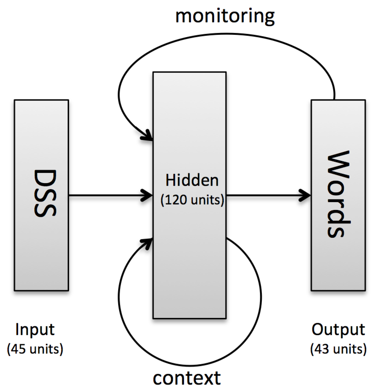
Our model architecture (see Figure 1) is broadly similar to the one of Frank et al. [23], with the main difference being that the inputs and outputs are reversed: it maps DSS representations onto sentences. As Frank et al. [23] point out, this is not intended to model human language development.
The model is an extension of a Simple Recurrent Network (SRN [31]). It consists of an input layer, a 120-units recurrent hidden (sigmoid) layer, and a 43-units (softmax) output layer. The dimensionality of the input layer is determined by the chosen semantic representation (150-dimensional situation vector or 44-dimensional belief vector), plus one bit indicating if the model should produce an active sentence (1) or a passive one (0). The output layer dimensionality is the number of words in the vocabulary plus the end-of-sentence marker (43).
Time in the model is discrete. At each time step t, the activation of the input layer is propagated to the hidden recurrent layer. This layer also receives its own activation at time-step (zeros at ) through context units. Additionally, the hidden layer receives the word produced at time-step (zeros at ) through monitoring units, where only the unit corresponding to the word produced at time-step is activated (set to 1).
We did not test with more sophisticated architectures such as LSTMs [32] or GRUs [33] because the focus of this work are the representations used by the model, rather than the model itself. Consequently, we tried to use the minimum machinery possible aside from the input and output representations.
More formally, activation of the hidden layer is given by:
where is the weight matrix connecting the input layer to the hidden layer, connects the hidden layer to itself, connects the monitoring units to the hidden layer, and is the bias unit of the hidden layer.
Then, the activation of the hidden layer is propagated to the output layer, which yields a probability distribution over the vocabulary, and its activation is given by:
where is the weight matrix connecting the hidden layer to the output layer and is the output bias unit.
The word produced at time-step t is defined as the one with highest probability (highest activation). The model stops when an end-of-sentence marker (a period) has been produced.
While it is outside the scope of this work, Calvillo and Crocker [34] presents a more thorough analysis of the internal mechanism of this model using Layer-wise Relevance Propagation [35].
As an example, Figure 2 illustrates the production of “someone plays badly.”. At time step , the DSS representation is fed to the hidden layer, which propagates its activation to the output layer. The output layer then yields a probability distribution over the vocabulary. In this case, the words “someone” and “a” have high activation. Since “someone” has the highest activation, it is the word the model produces. At , the hidden layer is fed again with the DSS representation, but this time also the activation of the hidden layer at and the word produced at (“someone”). It then propagates its activation to the output layer, which again yields a probability distribution over the vocabulary. This time the only activated word is “plays”. At , the process is repeated but this time the model activates “badly” and “a”. Since ”badly” has higher activation, it produces “badly”. Finally, at , the model produces “.”, which signals the end of production.
Testing for Systematicity
We defined different test conditions where the model must produce a sentence that it has not seen during training. Depending on its success, and how different the test items are to the training ones, we can assess the degree to which the model can generalize and exhibit systematicity.
The model was trained with cross-entropy backpropagation [36] and stochastic gradient descent (see Appendix B for more details). Each test instance corresponds to giving the model a and seeing whether the model can produce one of the related sentences in . The test conditions are divided into three sets corresponding to the next three sections: the first set (Active vs. Passive) tests whether the model can produce sentences in passive or active voice for a novel semantics. The second set (Words in New Syntactic Roles) tests whether the model can produce a word in a syntactic role with which that word was not seen in training. Finally, the third set (Semantic Anomalies) tests whether the model can produce sentences for situations that violate rules of the microworld.
4. Active vs. Passive
The dataset contains 782 unique DSS representations of microworld situations. These were divided in two sets: setAP () are situations related to both active and passive sentences, and setA () are situations related only to active sentences in which the direct object is a person (e.g., “Heidi beats Charlie.”) or unspecified (e.g., “Charlie plays.”), for which the microlanguage defines no passive sentences. Using this division, we defined our test conditions, which are outlined in Table 4.
setAP allowed for three conditions:
- 1: The model has seen active sentences, and a passive is queried.
- 2: The model has seen passive sentences, and an active is queried.
- 3: New situations, passive and active sentences are queried.
setA allowed for two testing conditions:
- 4: The model has seen active sentences, and a passive is queried.
- 5: New situations, passive and active sentences are queried.
These conditions correspond to different levels of generalization. In all cases, the queried sentence is new to the model. For Conditions 1, 2 and 4 the model has seen the situations but not in the queried voice. Importantly, for Conditions 3 and 5, the model has never seen the situation itself.
From another view, in Conditions 1, 2 and 3, the model has seen similar syntactic and semantic patterns but not the specific sentences or semantics. In contrast, in Conditions 4 and 5, where a passive is queried, the model must produce a sentence with a voice for which no example was given during training, not only for that specific semantics but for that type of semantics.
For these conditions, we applied 10-fold cross-validation, where for each fold, some items are held out for testing, and the rest are used for training. Thus setAP was randomly shuffled and split into 10 folds of 90% training and 10% test situations, meaning per fold 382/42 training/test items. For each fold, the test situations were further split into the three conditions, rendering 14 different test situations per condition, per fold. SetA was also shuffled and split into 10 folds, but in order to preserve uniformity, for each fold 14 situations were drawn per condition, meaning that each fold contained 28 test and 330 training situations.
For Condition 1, the situations were coupled with their active sentences and incorporated into the training set (while the passive sentences remained in the test set) and vice versa for Condition 2. Similarly, for Condition 4 the active sentences were incorporated into the training set, while during testing the model will be queried for a passive construction.
For each type of semantic representation (150-dimensional situation vectors and 44-dimensional belief vectors), we trained 10 instances of the model initialized with different weights, corresponding to each fold as described above. The results reported below are averages over these instances.
The model was first tested to see if it could produce a single sentence for each test item. Then, the model was tested to see whether it could produce all the sentences related to each test item.
4.1. Quantitative Analysis
As initial production policy, we define the word that the model produces at each time step as the one with the highest activation in the output layer. Thus, for a , the model produces a sentence describing the state-of-affairs represented in .
We assume that is correct if it belongs to the set of all possible realizations of in the queried voice. However, sometimes does not perfectly match any sentence in . As such, we compute the similarity between , and each sentence in , using their Levenshtein distance [37]; which is the number of insertions, deletions or substitutions that are needed in order to transform one string into another. More formally, Levenshtein similarity between sentences and is:
where is the Levenshtein distance. This similarity is 0 when the sentences are completely different and 1 when they are the same. Then, having a sentence produced by the model , we compute the highest similarity that one can achieve by comparing with each sentence s in :
For each test item, the model produced a sentence , which was compared to the expected ones, rendering the results in Table 5. For Conditions 4 and 5, where the model is queried a passive sentence, there are no corresponding examples in the dataset.
The performance using the 150-dimensional situation vectors can be seen in columns 3 and 4 in Table 5. On average, the model produces perfect sentences for almost two thirds of the situation vectors. While this may seem modest, we should consider that the situation vectors went through a dimensionality reduction, after which some information is lost. Nevertheless, the model achieves a similarity score on the test conditions. Since all sentences generated are novel to the model, this demonstrates the model can reasonably generalize.
For Condition 5 where active sentences are queried, we see a drop of performance. This could be because setA contained fewer sentences per situation and therefore fewer training items.
The performance with belief vectors can be seen in the last two columns in Table 5. The average similarity across all the test conditions is ( of perfect matches), which is very high and almost perfect in several cases, demonstrating high semantic systematicity.
Given that the errors with belief vectors are much fewer, and that a qualitative analysis (in the next subsection) shows that the sentences are similar in nature, we continue the rest of this quantitative analysis using only belief vectors.
Now we test whether the model can produce not only one sentence but all the sentences related to a given situation. Previously, at each time step the word produced was the one with highest activation. Sometimes, however, multiple words can have high activation, particularly when they all may be correct continuations of the sentence. In order to explore these derivations, we redefine the word production policy: at a given time step, the words produced are all the words with an activation above a threshold . By following all the word derivations that comply with this, the model can produce multiple sentences for a given semantics.
In general, should be low enough such that the model can derive the range of possible sentences but not too low so as to avoid overgenerations. We evaluated in terms of precision and recall several formulations of in order to identify the one that reproduces better all and only the sentences related to the semantic representations in the training set. The results indicate that is rather insensitive to the shape of the output distribution and that a fixed value may be sufficient (see Appendix C for further details). Indeed, a maximum f-score value of was achieved setting .
For our experiments, we set , which has a high recall () and a relatively high precision (). A high recall is preferred in order to produce a relatively large number of sentences that could give us insight into the production mechanism of the model.
For each condition, the following was done: for each , we calculated precision, recall and f-score of the set of sentences produced by the model with respect to the set ; then, these values were averaged across the representations of the test condition. In these calculations, only the sentences that fully matched a sentence in were considered, discarding partial matches. Finally, these values were averaged across the previously described 10 folds, giving the results in Table 6.
The first and second columns in Table 6 show the test conditions and the type of sentence the model must produce. The third column shows the average number of sentences related to its standard deviation. For example, in Condition 2, each is related to () active sentences. In general, the range is quite wide: some representations are related to one sentence, while others are related to many more, 130 being the maximum. On average, the model must produce () encodings per .
The fourth column in Table 6 shows the percentage of situations where the model produced all expected sentences without errors, which was the case for more than half of the representations in all conditions (55.9% on average). Considering only these cases, the mean number of sentences per situation was (), showing that the model can reproduce a large number of sentences per semantics without difficulties, sometimes reproducing up to 40 different encodings without errors.
The last three columns in Table 6 show precision, recall and f-score. In all conditions the model produced more than 90% of the expected sentences (93.7% on average). Additionally, the sentences produced were mostly correct (80.8% on average). The value of was chosen such that recall would be high; nonetheless, as we will see shortly, the sentences overgenerated are semantically very similar to the ones expected, raising again the question of whether they should be considered errors.
From these results, we see that for more than a half of the situations, the model can perfectly produce all the related sentences, and even for the situations with errors, the model can reproduce a large proportion of the expected sentences, even if they are novel, again demonstrating systematicity.
4.2. Qualitative Analysis
As before, we analyze first the model’s output in single sentence production, and then we continue with the case where the model must produce all the sentences related to a semantics.
Inspecting the sentences produced with the two types of representations (situation and belief vectors), we see that in both cases they are, with only few exceptions, syntactically correct and in all cases their semantics are, if not fully correct, at least closely related to the intended semantics.
The dimensionality reduction used to generate the 150-dimensional situation vectors introduces some information loss: the sentences with adverbial modifiers do not distinguish between “well” and “badly” and between “ease” and “difficulty”. The errors elicited for three folds were manually analyzed, finding that out of 82 errors, 34 () were related to modification. The information loss affects also other aspects, causing other error types but with fewer attestations.
Belief vectors elicited no errors related to adverbial modification. Without these errors, the sentences obtained using the two kinds of representations are qualitatively similar. Because of that, and since the errors with belief vectors are much fewer, we focus the rest of the analysis on the output obtained using belief vectors. However, we expect the performance using the 150-dimensional situation vectors would be similar to the one using belief vectors if the dimensionality reduction did not introduce information loss. See [38] for an alternative dimensionality reduction technique that may well mitigate this loss.
Although the performance with belief vectors is quite high, the model still produces systematic errors that provide us with insight into its internal mechanism. Because of that, the errors produced in five folds were manually inspected to see their regularities. Examples of these are in Table 7.
All the inspected errors occur when the model produces a sentence that is semantically very similar to the one expected, reproducing patterns of the speech error literature (e.g., [39]), which states that speech errors involve elements with phonological and/or semantic similarity. In our case, the model does not operate with phonological information, and consequently the errors are solely related to semantic similarity. This pattern appears even when testing with training items, where the model cannot distinguish between some highly similar situations, even though it has already seen them (Examples 1–3 in Table 7).
The errors observed (35 in total) can be classified into three main categories:
- Underspecification (): sentences providing correct information but omitting details (Examples 4–6 in Table 7).
- Overspecification (): sentences with information that is not contained in the semantics but that is likely to be the case (Examples 7–9 in Table 7).
- Very high similarity (): errors related to situations that are remarkably similar because of the design of the microworld (Examples 10–12 in Table 7).
The model is expected to describe situations assuming that the comprehender has no contextual information. Thus, a sentence that underspecifies gives less than enough information to fully describe the intended situation, while a sentence that overspecifies gives more information than what the semantics contains. It is debatable whether these should be considered as errors, given that people are not as precise, sometimes being vague (underspecifying) and sometimes making assumptions under uncertainty (overspecifying). For uniformity, however, we consider an “error” any difference between the semantics of the input and the semantics of the sentence produced.
The errors in the third category are sentences that seem correct at first glance; it is only after looking deeply into the microworld and the microlanguage that we see the error. First, in this microworld, whenever there is a winner, there is also a loser, meaning that sentences that are apparently contradictory (“someone loses.” vs. “someone wins.”) actually have the same implications and therefore are semantically identical. Second, the winner and the loser are usually in the same location, except when playing hide and seek, in which case the loser can be in the bedroom, while the winner could be in the bathroom and vice versa. Finally, prepositional phrases (e.g., “in the bedroom”) are attached to the subject of the sentence according to the microlanguage, meaning that in “Heidi beats Sophia in the bedroom”, Heidi is in the bedroom while Sophia could be in either the bedroom or the bathroom; similarly, in “Sophia loses to Heidi in the bedroom”, it is Sophia who stays in the bedroom while Heidi could also be in the bathroom. Apart from this detail, the situations are almost identical.
So far we see the model can take the linguistic elements learned during training in order to characterize situations for which it has no experience. The only difficulty appears to be the distinction of highly similar situations. However, the performance is very good in general and even for the sentences with an error, the output is largely correct. Furthermore, these errors serve to further demonstrate systematicity, as they are elicited precisely because of proximity/similarity in the semantic space, where similar situations have representations that are close to each other.
We also analyzed manually the output for three folds when the model must produce all the sentences related to each semantics. We found 391 sentences with errors, which followed the same patterns and proportions as in single sentence production. Additionally, since the model explores areas of low probability, a fourth category of errors appeared, which interestingly seems to coincide with errors found in the literature about human speech errors, such as repetitions and substitutions [40]; and only four sentences had a clear syntactic anomaly.
In general, the sentences produced with the most activated words are the best, and as one goes further away from the most activated words, errors start to appear, first producing underspecification/overspecification and then repetitions or syntactic errors. Nonetheless, with only few exceptions, the sentences maintain syntactic adequacy and high semantic similarity.
Finally, when the model produces multiple sentences we can also identify undergenerations, which show what the model preferred not to produce. We compared the undergenerated sentences, in the same three folds as before, against the ones produced. We found 38 situations with undergenerated sentences, which in general followed the statistical patterns of the microlanguage. For example, the location is preferred to be mentioned at the end. For more details, see Appendix D.
4.3. Undefined Passive Sentences
For Conditions 4 and 5, where a passive sentence is queried, Table 8 presents examples of output sentences and the situations that they were supposed to convey. These situations can be of two types: the first one involving a winning/losing situation where both actors are explicitly mentioned, and the second type being situations where the object of the action is unspecified.
We report the case where the model must produce multiple sentences per semantics, because it gives us a slightly wider view; however, the results are very similar for single sentence production. As before, we manually analyzed the output for three folds.
Here, the model must produce passive sentences for areas in the semantic space to which no sentences in the microlanguage are related. Consequently, the model is more uncertain, activating at each time step more words, producing relatively more sentences. Most of these follow the semantics; however, productions with low probability contain errors similar to those previously reported.
Concerning winning/losing situations (77 situations, Examples 1–2 in Table 8), the object is always a game because in the microworld winning/losing only happens when playing games. Thus, the model produces the name of the game when it is known (e.g., “soccer is…”), otherwise the sentence starts with “a game is…”. Then, one player is mentioned (one omitted) and the rest of the situation is described.
For situations with an unspecified object (seven situations, Examples 3–4 in Table 8), it is unknown whether the subject is playing a game or with a toy. Most of the time (four situations), both types of sentences are produced: sentences where “a game” is the object, and sentences where “a toy” is the object. Apart from this, the sentences follow the semantics.
Similar to the other conditions, over and underspecification errors occur in Conditions 4 and 5, but are rare (, Example 5 in Table 8). Two types of error that appear only for these situations are the inversion of the winning/losing relation in game situations (39 situations, Example 6 in Table 8) and the mention of the agent at the beginning of the sentence (12 situations, Example 7 in Table 8).
Although the model exhibits confusion as it explores areas of low probability, it can still process most information of each input. For these conditions, not only the specific representations are novel but also the model has never seen this kind of situation coupled with passive sentences. It is because of the systematic behavior of the model that it can produce coherent sentences for these areas of the semantic space. A classical symbol model would have difficulties producing any output, as the grammar rules describing passive sentences for these situations are simply non-existent in this microlanguage. From this view, our model can be regarded as more robust and perhaps even more systematic.
5. Words in New Syntactic Roles
The second set of test conditions investigates whether the model can produce words in syntactic positions relative to a verb to which they were not related during training. For example, the model may have seen sentences where the object of “plays” is “soccer” or “hide_and_seek”, and we test whether the model can produce “Charlie plays chess.”, where ”chess” has never been seen as the object of “plays”. Thus, while the model has seen the target syntactic patterns, it has never seen them related to the specific target words. More concretely, the model must produce the name of a game in the following syntactic positions:
- Condition 6—Direct Object of “plays”: e.g., having as target “chess”, in training the model sees sentences such as “someone plays soccer” or “someone wins at chess”, but not “someone plays chess”.
- Condition 7—Prepositional Object of “loses”: e.g., having as target “chess”, in training the model sees sentences such as “someone loses at soccer”, “someone loses in the playground”, but not “someone loses at chess”.
- Condition 8—Subject of “plays”in passive sentences: e.g., having the target “chess”, the model sees during training “hide_and_seek is played…” or “chess is lost…”, but not “chess is played ”.
The targets are game names that differ, among other aspects, in the degree to which they are necessary. For example,“Charlie plays in the street.” implies the game is soccer because that is the only game that can be played in the street. Therefore, “soccer” can always be omitted because the street is also the only place where soccer can be played. Conversely, chess can be played only in the bedroom, which is a place where hide and seek can also be played; therefore, it is always necessary to name chess. Hide and seek can be played everywhere except in the street, and it is the only game that can be played in the playground and the bathroom. Therefore, one can omit naming hide and seek in the bathroom and playground but not in the bedroom. In sum, naming soccer can always be omitted, chess is always necessary and hide and seek can be omitted depending on the location.
For each condition and target, a training/test set is created, where the test set contains all semantic representations related to at least one sentence with the target pattern, while the training set contains the rest of the representations.
Results
The model produced multiple sentences for each test item, having , as before. We assume the model produced the target if one of the produced sentences contained the target pattern and conveyed correctly the semantics. For each condition and target, 10 instances with different weight initializations were trained. The results reported in Table 9 are averages over them.
Column 7 in Table 9 shows the percentage of times the model produced the target for each condition. For the cases where the target pattern is necessary (the semantics cannot be conveyed through other linguistic structures), columns 3 and 4 show the number of test items and the corresponding percentage in which the model correctly produced the target pattern. Similarly, columns 5 and 6 show the number of items and the percentage in which the model produced correctly the target pattern for cases in which the pattern is not necessary, as the semantics can be conveyed through other linguistic structures.
The low scores in condition 7 and hide and seek are because those are the situations with high semantic similarity as before. Here the model has seen in training sentences of the form ”X beats Y at hide_and_seek in the bedroom”, which are very similar to ”Y loses at hide_and_seek in the bedroom” but not the same, as explained before. Due to this confusion, the model produces wrong sentences, avoiding the target pattern.
The difference between columns 5 and 7 shows a tendency to produce the target pattern more when there are no alternative ways to encode the semantics. Indeed, in the absence of competing encodings, the model should be able to explore and produce words in areas of low probability related to unseen structures. Consequently, for the production of a novel structure, there should be few competing alternatives, as the model prefers the more frequent or already seen encodings.
We see variation depending on whether the target is necessary to encode the situation or the game that is being played. However, in most conditions, the model can still produce the target pattern for more than 85% of the situations, showing that the model could produce words in syntactic positions with which they were not related during training.
6. Semantic Anomalies
The last test condition investigates whether the model can produce sentences for semantic representations that violate rules of the microworld. These representations are not only outside of the training set but also outside of the set of possible elements in the input space. Intuitively, this condition addresses the human ability to produce sentences for situations that are not real or in contradiction to common world knowledge [41].
According to the rules of the microworld, each game is played only in specific locations: chess in the bedroom, soccer in the street, and hide and seek in all locations except in the street. We constructed representations that violate these rules by taking the semantic representations related to the sentences with the pattern "X plays Y" where X is a person and Y is a game. Then, we set to 0 all dimensions related to locations (basic events of the form where Z is a location that is not the target one). Finally, the target location (which violates the rules) is set to 1.0 for the protagonist of the situation (X). In this way, the original semantic representations are mostly preserved, except that all people are placed in the target location.
For example, the representation for “Charlie plays chess in the playground.” is the same as the one for “Charlie plays chess in the bedroom.”, except that the dimensions related to locations would place “Charlie” in the playground and would remove all activation related to other people in other places.
Here, the training set is the full dataset, and the test items are the newly created representations that violate the rules. We trained three instances of the model and manually analyzed their output.
Results
The sentences produced show that the model is uncertain about the meaning of the input. In most cases the model produces the usual place for the game (bedroom for chess, street for soccer), or in the case of hide and seek, the model avoids expressing the location. In all cases, the sentences produced follow the rules of the microworld and avoid aspects that would contradict those rules.
During training, the model learns, for example, that soccer is always played in the street, so if someone is playing soccer, he/she is in the street. Then, if a semantics indicates that someone plays soccer in the playground, according to the microworld, either that person is not playing soccer or he/she is in the street. The sentences produced follow one of these options but not both.
It is debatable whether these outputs are correct or not. If we consider the microworld rules as unbreakable, then the model is correct avoiding sentences that make no sense in this microworld. However, if we consider that the semantic representation should be followed, no matter the implications in the microworld, then the model was incorrect as it was unable to follow those representations.
If we expect the model to produce sentences that break the rules, then perhaps we need to relax those rules. In the real world, some events imply certain other events; however, most events are independent of each other. Moreover, a person’s knowledge is limited, and one cannot form very strong rules about the world, since for each rule, many exceptions exist. In contrast, with the limited set of events that the model experiences, the rules that the model learns could be considered as “hard”, as during training, it receives no information leading to believe that those rules can be broken.
We should also consider that the dimensions in the semantic representations are not independent. Indeed, each game entails certain locations. We altered the values of the location dimensions, but the model still knows the game, which implies different locations, and which can potentially cancel the effect of our alterations. If we wish the model to produce sentences breaking these entailments, it would need to be rewired such that each input dimension is independent, and thus, altering one dimension would not affect the model’s behavior with respect to the others.
7. Discussion
7.1. Semantic Systematicity
Given the wide success of artificial neural networks in contemporary systems of computer vision and natural language processing, among other applications (e.g., [42]), it is evident that artificial neural networks can generalize. Nonetheless, here we address semantic systematicity, which is argued to be a sign of human-level systematicity [14,15], and to this date it is still not clear to what extent connectionist approaches can achieve it. If a connectionist model shows semantic systematicity, it would mean that connectionist architectures are capable of human-level systematicity, and therefore, they can be plausible models of human cognition.
We approached this from a sentence production perspective, presenting a model that learns to produce sentences from DSS representations, generalizing to novel sentences and situations. In all test conditions, the model could produce new combinations of words that follow the syntactic patterns of the microlanguage, while being coherent with the input semantics, thereby showing syntactic generalization. Crucially, the model also achieves semantic generalization, as demonstrated in test conditions 3 and 5, where the model was fed with novel semantic representations, so any correct output can be regarded as arising from the regularities within the microworld from which the DSS representations are derived—cf. the comprehension results by Frank et al. [23].
In Conditions 4 and 5, where a passive sentence is queried but the microlanguage does not define such structures, we see a behavior that could not be addressed by a classical symbolic model, at least not intuitively. A symbolic model operates over discrete symbols using symbolic rules that work in a predefined and precise way. Such a model would find difficulties with items that do not fit into any of the discrete and predefined symbolic units, and furthermore, it would not be able to process combinations of symbols that are not defined by any of the predefined rules. In other words, a symbolic model would be able to show a perfect combinatorial behavior but would be unable to handle representations for which no symbolic rule is defined. The model proposed here does not have that issue; it can also operate over discrete units, in this case words, but the semantic space is continuous, where unknown areas can still be interpreted. As one can see, the sentences produced by the model for these conditions are in general semantically and syntactically correct.
The fact that difficulties arise encoding highly similar situations suggests that the model can reconstruct the topography of the semantic space, clustering situations that are related. At the same time, the model assigns linguistic structures to each area in this space such that semantically similar situations are assigned linguistically similar realizations. Since the semantic space is continuous, in theory the model should be able to generate sentences for unseen areas as long as it is given enough information during training in order to reconstruct the semantic space and the mapping between semantics and linguistic realizations, as proposed by Frank et al. [23].
The results show that this is indeed the case. Conditions 1 and 2 demonstrated the model can generate sentences for semantically known situations but with a different voice (active/passive), showing syntactic systematicity. Conditions 3 and 5 demonstrated that the model can generate sentences for unseen areas in the semantic space, thus showing semantic systematicity. Conditions 4 and 5, where passive sentences are queried, demonstrated that the model is able to produce coherent sentences even if the grammar that was used to build the dataset does not associate passive constructions to these situations. Furthermore, the model is not only able to produce a single novel sentence for a novel semantic representation, but it can also produce most (if not all) of the sentences that are related to a given semantics.
Regarding the production of words in novel syntactic roles, our model showed a lower performance; however, it was still able to produce the expected patterns in the majority of the situations. We saw that the presence of competitors reduced the percentage of times the model produced the expected patterns; this might be related to the form of the softmax activation function of the output layer, which normalizes the activations. We leave to future work experiments where the output units are independent of each other.
Finally, regarding the production of sentences describing situations that violate the rules of the microworld, we saw that the model was unable to produce such sentences. In this case, it is possible that the structural regularities that permitted the model to generalize in the other conditions are the ones preventing the model from producing sentences that violate the rules of the microworld. We speculate that a microworld with less strict rules would generate representations where pairs of events that never or almost never co-occur are still interpretable by a neural network. We leave this scenario also for future work.
7.2. Systematicity Requirements
Theoretical analyses show that multilayer perceptrons are universal function approximators [43] and that recurrent neural networks are at least as powerful as a Turing Machine [44,45]. Then, the problem of systematicity is not about computational power but about learning. While a set of connection weights with systematicity exists for any function, the difficulty to learn such weights depends on different factors, such as the complexity of the function, the input/output spaces and the representations that are used.
Without discarding the impact that certain architectures have on facilitating generalization, we recognize some conditions of the input and output representations that are necessary and that could index the difficulty for learning a particular behavior.
A first condition is that the representations must contain information about what is represented, such that the model can draw relations with other representations, whether seen or not. Analogous representations, as the ones used here, show and depend on the nature of what they represent, where relations among items are apparent in their representations (see [23]). Thus, similar entities have similar representations.
A related aspect is informativity. A representation is informative if it contains the information necessary for the task. The 25,000-dimensional situation vectors defined by Frank et al. [23] contain very detailed information; however, after the dimensionality reduction used to create the 150-dimensional situation vectors, some aspects are lost, reducing the performance of the model. In turn, belief vectors also do not contain as detailed information as the original 25,000-dimensional situation vectors, only representing averages over observations. In both cases there is information loss; nonetheless, the belief vectors still contained the required information.
Another condition is that the input space has to be structured, such that regularities in the training set can be used to recognize new instances. In other words, the nature of an item should be interpretable by looking at items in the spatial vicinity. If the input space is too erratic, the model would have difficulties interpreting inputs in new areas.
The space of input representations of our model, which is defined by all possible combinations of basic events, is structured in the sense that some pairs of basic events always co-occur, some are not allowed and some others co-occur with certain probabilities. These regularities are recognized in training, allowing the model to infer information about unseen events.
The last condition we recognize is that the function to be learned should be predictable with respect to the input space, such that the processing for an input can be inferred by looking at the processing for similar inputs. In other words, similar inputs should be processed similarly.
In our case, the output sentences have regularities as they were all constructed with the same grammar, defining a space where some constructions are allowed and some are not. These regularities allow the model to learn the syntactic patterns of the microlanguage. Furthermore, the mapping between semantic representations and sentences is such that similar semantic representations are processed similarly, as demonstrated by the errors performed by the model. These regularities in the mapping of inputs to outputs permitted the model to process correctly novel inputs.
In sum, for systematicity to be possible, the representations should be informative, items should be interpretable by looking at similar items and similar items should be processed similarly. As we saw, these requirements were met by our model’s inputs/outputs, which permitted a successful learning for most of our test conditions.
7.3. Recent Related Work
Although the systematicity debate has been ongoing for several decades, the relatively recent success of deep learning has brought interest again into this topic. As a result, several rule-based generated datasets have been proposed to test and measure compositional generalization (e.g., [46,47,48]).
Lake and Baroni [49] presented SCAN, which is a dataset where compositional navigation instructions (e.g., “jump twice”) are mapped to sequences of actions (e.g., “JUMP JUMP”), and where different training/test splits assess different types or levels of systematicity. This dataset has been extended [50,51] and used to test systematicity with several sequence to sequence RNN architectures (e.g., [49]) and convolutional neural networks [52]. Moreover, specially designed neural architectures have been proposed to solve some of the tests in SCAN [22,53], which are similar to the dual-path model of Chang et al. [26], separating syntax from semantics.
Gordon et al. [54] presents a permutation equivariant model that by design builds word embeddings such that words that are to be treated similarly (e.g., all verbs, or “left” and “right”) are linked to similar embeddings, even if during training they appear with a different distribution. This model achieves excellent performance in some of the test splits of SCAN.
An important difference between the methods used by recent studies and ours is that our task is not a sequence to sequence one where an encoder generates an intermediate representation of the input, which is later used by a decoder to generate the desired outcome. We focus on the second step, that is, the generation of a sentence given a semantics. In our case, the semantic space is constructed prior to training of the production model and therefore its structure is independent of the statistical properties of training/test splits. Thus messages that are to be treated similarly have similar representations even if during training they appear with different distributions, as in Gordon et al. [54].
Kim and Linzen [55] proposed COGS, which is a dataset that maps sentences to their logical form. COGS differs from SCAN in that the former is more focused on linguistics, containing different linguistic phenomena related also to different systematicity levels. An important difference between the DSS representations of Frank et al. [23] and COGS is that while they both map sentences to their semantics, the DSS representations are completely grounded on the microworld (the semantic representations of COGS are logical formulas), reflecting the regularities of the microworld, which we argue is important to achieve systematicity, as it provides structure to the semantic space.
Other ways in which systematicity has been approached is through sophisticated training methods such as data augmentation [56] and meta-learning [57,58].
The general conclusion of these studies is that systematicity is not a property that modern deep learning methods achieve by default (e.g., [21]), that some architectures and training methods help (e.g., [22,53,57]) and that some compositional tasks are more difficult than others (e.g., [55]). We aim to contribute to this topic by focusing on the importance of the representations themselves in achieving systematicity, perhaps in a similar way as Gordon et al. [54], and also by studying the opposite direction of semantic parsing: sentence production.
8. Conclusions
We presented a sentence production model that receives as input the distributed semantic representations of the Distributed Situation Space model (DSS, [23]). This model was tested to see first whether it could learn to produce sentences with these representations, showing that indeed that was the case. An error analysis revealed that the errors were related to highly similar situations, reproducing some findings of the speech error literature and reflecting the statistical patterns of the training set.
In addition, the model was tested to see whether it could exhibit systematicity. The results showed that the model could handle and produce novel sentences for novel message representations in several test conditions. Further, the model was able to produce passive sentences for areas in the semantic space for which the microlanguage does not define passive sentences, and also sentences with words in novel syntactic roles, exhibiting systematicity. Furthermore, the model could produce not only one sentence but most if not all of the sentences that were related to a particular semantics, demonstrating a systematic behavior.
The results of these tests were partly due to the architecture but more importantly to the semantic representations that were used as input for the model. These are points in a multidimensional continuous space, containing rich information about the situation that a sentence describes and reflecting the structure of the microworld from which they are derived.
Finally, we propose some conditions about the nature of the function to be learned and the representations used by a model in order to learn a particular function and exhibit systematicity. Namely, similar items should have similar informative representations, and thus they should also be interpreted and processed similarly. As we saw, these conditions were met by the function and the representations that we used, permitting the model to learn the expected behavior.
Author Contributions
Conceptualization, M.W.C., J.C. and H.B.; methodology, M.W.C., J.C. and H.B.; software, J.C. and H.B.; validation, J.C.; formal analysis, J.C.; investigation, J.C.; resources, J.C. and H.B.; data curation, J.C. and H.B.; writing—original draft preparation, J.C.; writing—review and editing, M.W.C. and H.B.; visualization, J.C.; supervision, M.W.C.; project administration, M.W.C.; funding acquisition, J.C and M.W.C. All authors have read and agreed to the published version of the manuscript.
Funding
This research was funded by the Deutsche Forschungsgemeinschaft (DFG, German Research Foundation)—Project-ID 232722074—SFB 1102. The first author was additionally supported by the National Science Foundation grant BCS-1734304 and the Mexican National Council of Science and Technology (CONACYT).
Institutional Review Board Statement
Not applicable.
Informed Consent Statement
Not applicable.
Data Availability Statement
The dataset as well as the code to train and test the sentence production model can be found here: https://github.com/iesus/systematicity-sentence-production (accessed on 11 August 2021).
Conflicts of Interest
The authors declare no conflict of interest. The funders had no role in the design of the study; in the collection, analyses, or interpretation of data; in the writing of the manuscript, or in the decision to publish the results.
Appendix A. Grammar of the Microlanguage
Variable denotes nouns; denotes verbs; VP=verb phrase; APP=adverbial/prepositional phrase; PP=prepositional phrase. Items in square brackets are optional.
Appendix B. Training Procedure
All weights on the projections between layers are initialized with random values drawn from a normal distribution . The weights on the bias projections are initialized to zero. The model is trained using cross-entropy backpropagation [36], where at each time step the model is expected to produce the word of the training sentence that corresponds to that time step. Weights are updated accordingly after each word in the sentence of each pair in the training set. Note that each item of this set consisted of a paired with one of the possible sentence realizations describing the state of affairs represented in . Hence, during each epoch, the model sees all the possible realizations of contained in the training set.
During training, the monitoring units are set at time t to what the model was supposed to produce at time (zeros for ). This reflects the notion that during training the word in the training sentence at time-step should be the one informing the next time step, regardless of the previously produced (and possibly different) word (teacher forcing, [59]). During testing, the monitoring units are set to 1.0 for the word that was actually produced and 0.0 everywhere else.
Training occurs for a maximum of 200 epochs. Each epoch consists of a full presentation of the training set, which is randomized before each epoch. An initial learning rate of is employed, which is halved each time there is no improvement of performance on the training set during 15 epochs. No momentum is used. Finally, training halts if the maximum number of epochs is reached or if there is no performance improvement on the training set over a 40-epoch interval.
Appendix C. Activation Threshold
A given threshold can be evaluated in terms of precision and recall while trying to obtain all and only the possible sentences given a semantics. In these terms, the following variations were tested:
- Fixed:
- Entropy:
- Ratio to Maximum:
where manipulates how strict the threshold should be for all situations, and is the probability (activation) of word w at the output layer. The first formulation sets a common threshold for all productions. The second one allows to change according to the distribution of activation across all words at a specific derivation point. Finally, the third formulation allows to change according to the activation of each word compared to the maximum word activation at that point.
These definitions of were used to produce multiple sentences for each semantic representation in the training set, manipulating the value of . For each , precision, recall and f-score of the set of sentences generated by the model were calculated, with respect to the set . Then, these values were averaged across the semantic representations in the training set. For these calculations, a sentence produced by the model was only considered if it was a perfect match with a sentence in , consequently discarding all partial matches.
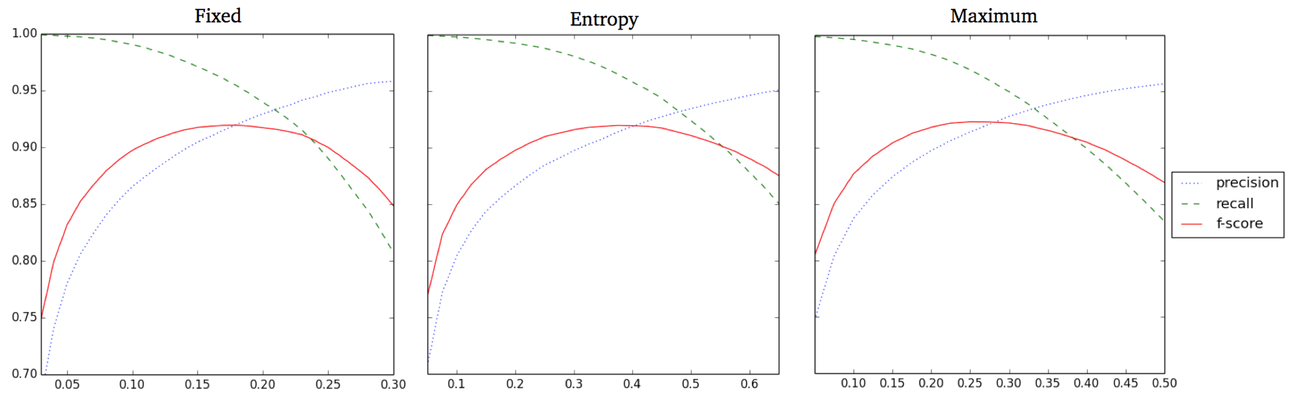
For each formulation and for each value of , Figure A1 shows average precision, recall and f-score averaging across the 10 folds used for Conditions 1-6. We see that the behavior is almost identical between the formulations, although in different scales. This suggests that the definition of is not sensitive to the form of the output distribution and that a global fixed threshold may be sufficient.
From Figure A1, we also notice that the model achieves a very high recall when setting to relatively low values. In this case, precision is rather low, but its value is still high enough to suggest that the model is heavily pruning the derivation forest to only the sentences that are related to the given semantics. Finally, we also see that the maximum f-score value is around , meaning that the model is able to a very high degree to reconstruct the whole set of training sentences.
Since the formulation of is rather stable, we set as a fixed threshold, and given the shape of the curve, we set it to the value of , which has a high recall () and a relatively high precision (). A high recall is preferred in order to produce a relatively large number of sentences that could give insight into the production mechanism of the model. This value was used for the multiple sentence production analyses.
Figure A1.
Precision, recall and f-score for different values of and for different formulations of on the training set.
Figure A1.
Precision, recall and f-score for different values of and for different formulations of on the training set.

Appendix D. Undergenerations
Undergenerations are sentences the model preferred not to produce, which we can judge in relation to those that were actually produced. Thus, the undergenerated sentences for three folds in multiple sentence production were compared against the ones produced. The undergenerations were related to 38 situations, following clear patterns:
- Overspecification Preferred (28 situations, 43 sentences, Examples 1–3 in Table A1): These sentences are correct and exact but they leave some aspects implicit. For example, “the boy plays well in the playground” implies that hide and seek is the game played because that is the only game that can be played in the playground. However, the model would prefer to say explicitly: “the boy plays hide_and_seek well in the playground. ”
- Underspecification Preferred (4 situations, 54 sentences, Example 4 in Table A1): The model prefers to be ambiguous, leaving details implicit. This happens rarely, producing “a girl” instead of “Sophia”, “someone” instead of “a girl” and “toy” instead “puzzle/jigsaw”.
- Constituent Order (16 situations, 110 sentences, Examples 5–7 in Table A1): Sentences with the same constituents but in different order. Location information is preferred at the end (13 situations, 48 sentences, Example 5 in Table A1), the model prefers to mention the winners first (3 situations, 62 sentences, Example 6 in Table A1), and there was an instance where “with ease” was preferred early.
- Winner/Loser Location (3 situations, 43 sentences, Example 8 in Table A1): Situations in which hide and seek is played inside, someone wins/loses and the location of the winner/loser is exchanged, producing only incorrect sentences.

Table A1.
Representative examples of undergeneration.
| Model’s Output | Undergenerated | |
|---|---|---|
| 1 | the boy plays hide_and_seek well in the playground. | the boy plays well in the playground. |
| 2 | a game is won with ease by someone in the bedroom. | a game is won with ease in the bedroom. |
| 3 | Charlie plays chess well in the bedroom. | Charlie plays chess well. |
| 4 | a girl plays inside with a puzzle. | Sophia plays inside with a puzzle. |
| 5 | the boy loses at soccer in the street. | the boy loses in the street at soccer. |
| 6 | Heidi beats Charlie at chess. | Charlie loses to Heidi at chess. |
| 7 | Charlie wins with ease at soccer. | Charlie wins at soccer with ease. |
| 8 | Heidi loses to Sophia in the bathroom. | Sophia beats Heidi in the bathroom. |
Regarding overspecification, the related linguistic patterns are more frequent. For example, naming the specific game can be omitted only when soccer is played in the street or hide and seek is played in the playground. The constituent order also follows the statistics of the language. For example, among all the sentences that contain “inside”/“outside”, mention it at the end. In general, the model’s preferences reflect the statistical properties of the training sentences.
References
- Chomsky, N. Syntactic Structures; De Gruyter Mouton: Berlin, Germany, 1957. [Google Scholar]
- Fodor, J.A.; Pylyshyn, Z.W. Connectionism and cognitive architecture: A critical analysis. Cognition 1988, 28, 3–71. [Google Scholar] [CrossRef]
- Fodor, J.A.; McLaughlin, B.P. Connectionism and the problem of systematicity: Why Smolensky’s solution doesn’t work. Cognition 1990, 35, 183–204. [Google Scholar] [CrossRef]
- Fodor, J.A. The language of thought; Harvard University Press: Cambridge, MA, USA, 1975; Volume 5. [Google Scholar]
- Marr, D. Vision: A Computational Investigation into the Human Representation and Processing of Visual Information; W. H. Freeman and Company: San Francisco, CA, USA, 1982. [Google Scholar]
- Symons, J.; Calvo, P. The Architecture of Cognition: Rethinking Fodor and Pylyshyn’s Systematicity Challenge; Chapter Systematicity: An Overview; MIT Press: Cambridge, MA, USA, 2014; pp. 3–30. [Google Scholar]
- Bechtel, W. The case for connectionism. Philos. Stud. 1993, 71, 119–154. [Google Scholar] [CrossRef]
- Gelder, T. Compositionality: A connectionist variation on a classical theme. Cogn. Sci. 1990, 14, 355–384. [Google Scholar] [CrossRef]
- Bodén, M. Generalization by symbolic abstraction in cascaded recurrent networks. Neurocomputing 2004, 57, 87–104. [Google Scholar] [CrossRef]
- Brakel, P.; Frank, S.L. Strong systematicity in sentence processing by simple recurrent networks. In Proceedings of the 31st Annual Conference of the Cognitive Science Society, Austin, TX, USA, 29 July–1 August 2009; pp. 1599–1604. [Google Scholar]
- Chang, F. Symbolically speaking: A connectionist model of sentence production. Cogn. Sci. 2002, 26, 609–651. [Google Scholar] [CrossRef]
- Elman, J.L. Distributed representations, simple recurrent networks, and grammatical structure. Mach. Learn. 1991, 7, 195–225. [Google Scholar] [CrossRef] [Green Version]
- Lake, B.M.; Ullman, T.D.; Tenenbaum, J.B.; Gershman, S.J. Building machines that learn and think like people. Behav. Brain Sci. 2017, 40, e253. [Google Scholar] [CrossRef] [Green Version]
- Hadley, R.F. Systematicity in connectionist language learning. Mind Lang. 1994, 9, 247–272. [Google Scholar] [CrossRef]
- Hadley, R.F. Systematicity revisited: Reply to Christiansen and Chater and Niklasson and van Gelder. Mind Lang. 1994, 9, 431–444. [Google Scholar] [CrossRef]
- Hadley, R.F.; Hayward, M.B. Strong semantic systematicity from Hebbian connectionist learning. Minds Mach. 1997, 7, 1–37. [Google Scholar] [CrossRef]
- Hadley, R.F.; Cardei, V.C. Language acquisition from sparse input without error feedback. Neural Netw. 1999, 12, 217–235. [Google Scholar] [CrossRef]
- Miikkulainen, R. Subsymbolic case-role analysis of sentences with embedded clauses. Cogn. Sci. 1996, 20, 47–73. [Google Scholar] [CrossRef]
- Jansen, P.A.; Watter, S. Strong systematicity through sensorimotor conceptual grounding: An unsupervised, developmental approach to connectionist sentence processing. Connect. Sci. 2012, 24, 25–55. [Google Scholar] [CrossRef]
- Farkaš, I.; Crocker, M.W. Syntactic systematicity in sentence processing with a recurrent self-organizing network. Neurocomputing 2008, 71, 1172–1179. [Google Scholar] [CrossRef]
- Baroni, M. Linguistic generalization and compositionality in modern artificial neural networks. Philos. Trans. R. Soc. 2020, 375, 20190307. [Google Scholar] [CrossRef] [PubMed] [Green Version]
- Russin, J.L.; Jo, J.; O’Reilly, R.C.; Bengio, Y. Systematicity in a Recurrent Neural Network by Factorizing Syntax and Semantics. In Proceedings of the 42nd Annual Conference of the Cognitive Science Society, Austin, TX, USA, 29 July–1 August 2020. [Google Scholar]
- Frank, S.L.; Haselager, W.F.; van Rooij, I. Connectionist semantic systematicity. Cognition 2009, 110, 358–379. [Google Scholar] [CrossRef] [Green Version]
- Frank, S.L.; Koppen, M.; Noordman, L.G.; Vonk, W. Modeling knowledge-based inferences in story comprehension. Cogn. Sci. 2003, 27, 875–910. [Google Scholar] [CrossRef]
- Zwaan, R.A.; Radvansky, G.A. Situation models in language comprehension and memory. Psychol. Bull. 1998, 123, 162–185. [Google Scholar] [CrossRef]
- Chang, F.; Dell, G.S.; Bock, K. Becoming syntactic. Psychol. Rev. 2006, 113, 234. [Google Scholar] [CrossRef] [Green Version]
- Mayberry, M.R.; Crocker, M.W.; Knoeferle, P. Learning to attend: A connectionist model of situated language comprehension. Cogn. Sci. 2009, 33, 449–496. [Google Scholar] [CrossRef] [Green Version]
- Brouwer, H. The Electrophysiology of Language Comprehension: A Neurocomputational Model. Ph.D. Thesis, University of Groningen, Groningen, The Netherlands, 2014. [Google Scholar]
- St John, M.F.; McClelland, J.L. Learning and applying contextual constraints in sentence comprehension. Artif. Intell. 1990, 46, 217–257. [Google Scholar] [CrossRef]
- Venhuizen, N.J.; Hendriks, P.; Crocker, M.W.; Brouwer, H. Distributional formal semantics. Inf. Comput. 2021, 104763. [Google Scholar] [CrossRef]
- Elman, J.L. Finding structure in time. Cogn. Sci. 1990, 14, 179–211. [Google Scholar] [CrossRef]
- Hochreiter, S.; Schmidhuber, J. Long short-term memory. Neural Comput. 1997, 9, 1735–1780. [Google Scholar] [CrossRef]
- Cho, K.; van Merrienboer, B.; Gülçehre, Ç.; Bougares, F.; Schwenk, H.; Bengio, Y. Learning Phrase Representations using RNN Encoder-Decoder for Statistical Machine Translation. arXiv 2014, arXiv:1406.1078. [Google Scholar]
- Calvillo, J.; Crocker, M. Language production dynamics with recurrent neural networks. In Proceedings of the Eight Workshop on Cognitive Aspects of Computational Language Learning and Processing, Stroudsburg, PA, USA, 19 July 2018; pp. 17–26. [Google Scholar]
- Bach, S.; Binder, A.; Montavon, G.; Klauschen, F.; Müller, K.R.; Samek, W. On pixel-wise explanations for non-linear classifier decisions by layer-wise relevance propagation. PLoS ONE 2015, 10, e0130140. [Google Scholar] [CrossRef] [PubMed] [Green Version]
- Rumelhart, D.E.; Hinton, G.E.; Williams, R.J. Learning representations by back-propagating errors. Nature 1986, 323, 533–536. [Google Scholar] [CrossRef]
- Levenshtein, V.I. Binary Codes Capable of Correcting Deletions, Insertions, and Reversals. Soviet Physics-Doklady 1966, 10, 707–710. [Google Scholar]
- Venhuizen, N.J.; Crocker, M.W.; Brouwer, H. Expectation-based Comprehension: Modeling the Interaction of World Knowledge and Linguistic Experience. Discourse Process. 2019, 56.3, 229–255. [Google Scholar] [CrossRef] [Green Version]
- Meringer, R.; Mayer, K. Versprechen und Verlesen. Eine Psychologisch-Linguistische Studie.([With the Assistance of] Carl Mayer.) New Edition with an Introductory Article by Anne Cutler and David Fay; John Benjamins Publishing: Amsterdam, The Netherlands, 1895; Volume 2. [Google Scholar]
- Clark, H.H.; Clark, E.V. Psychology and Language: An introduction to Psycholinguistics; Harcourt College Pub: San Diego, CA, USA, 1980. [Google Scholar]
- Hampton, J. The combination of prototype concepts. In The Psychology of Word Meanings; Schwanenflugel, P., Ed.; Psychology Press: New York, NY, USA, 1991. [Google Scholar]
- LeCun, Y.; Bengio, Y.; Hinton, G. Deep learning. Nature 2015, 521, 436. [Google Scholar] [CrossRef]
- Cybenko, G. Approximation by superpositions of a sigmoidal function. Math. Control. Signals Syst. 1989, 2, 303–314. [Google Scholar] [CrossRef]
- Siegelmann, H.T.; Sontag, E.D. On the computational power of neural nets. J. Comput. Syst. Sci. 1995, 50, 132–150. [Google Scholar] [CrossRef] [Green Version]
- Siegelmann, H.T. Neural Networks and Analog Computation: Beyond the Turing Limit; Springer Science & Business Media: Berlin/Heidelberg, Germany, 2012. [Google Scholar]
- Keysers, D.; Schärli, N.; Scales, N.; Buisman, H.; Furrer, D.; Kashubin, S.; Momchev, N.; Sinopalnikov, D.; Stafiniak, L.; Tihon, T.; et al. Measuring compositional generalization: A comprehensive method on realistic data. arXiv 2019, arXiv:1912.09713. [Google Scholar]
- Sinha, K.; Sodhani, S.; Dong, J.; Pineau, J.; Hamilton, W.L. CLUTRR: A diagnostic benchmark for inductive reasoning from text. arXiv 2019, arXiv:1908.06177. [Google Scholar]
- Yanaka, H.; Mineshima, K.; Inui, K. SyGNS: A Systematic Generalization Testbed Based on Natural Language Semantics. arXiv 2021, arXiv:2106.01077. [Google Scholar]
- Lake, B.; Baroni, M. Generalization without systematicity: On the compositional skills of sequence-to-sequence recurrent networks. In Proceedings of the 35th International Conference on Machine Learning, Stockholm, Sweden, 10–15 July 2018; pp. 2873–2882. [Google Scholar]
- Loula, J.; Baroni, M.; Lake, B.M. Rearranging the familiar: Testing compositional generalization in recurrent networks. arXiv 2018, arXiv:1807.07545. [Google Scholar]
- Bastings, J.; Baroni, M.; Weston, J.; Cho, K.; Kiela, D. Jump to better conclusions: SCAN both left and right. arXiv 2018, arXiv:1809.04640. [Google Scholar]
- Dessì, R.; Baroni, M. CNNs found to jump around more skillfully than RNNs: Compositional generalization in seq2seq convolutional networks. arXiv 2019, arXiv:1905.08527. [Google Scholar]
- Li, Y.; Zhao, L.; Wang, J.; Hestness, J. Compositional generalization for primitive substitutions. arXiv 2019, arXiv:1910.02612. [Google Scholar]
- Gordon, J.; Lopez-Paz, D.; Baroni, M.; Bouchacourt, D. Permutation Equivariant Models for Compositional Generalization in Language. International Conference on Learning Representations. 2019. Available online: https://openreview.net/pdf?id=SylVNerFvr (accessed on 13 August 2021).
- Kim, N.; Linzen, T. COGS: A compositional generalization challenge based on semantic interpretation. arXiv 2020, arXiv:2010.05465. [Google Scholar]
- Andreas, J. Good-enough compositional data augmentation. arXiv 2019, arXiv:1904.09545. [Google Scholar]
- Conklin, H.; Wang, B.; Smith, K.; Titov, I. Meta-Learning to Compositionally Generalize. arXiv 2021, arXiv:2106.04252. [Google Scholar]
- Lake, B.M. Compositional generalization through meta sequence-to-sequence learning. arXiv 2019, arXiv:1906.05381. [Google Scholar]
- Williams, R.J.; Zipser, D. A Learning Algorithm for Continually Running Fully Recurrent Neural Networks. Neural Comput. 1989, 1, 270–280. [Google Scholar] [CrossRef]
Figure 1.
Model architecture.

Figure 2.
Example of sentence production: “someone plays badly.”

Table 1.
Concepts in the microworld of Frank et al. [23].
Table 1.
Concepts in the microworld of Frank et al. [23].
| Class | Variable | Class Members (Concepts) | # |
|---|---|---|---|
| People | p | charlie, heidi, sophia | 3 |
| Games | g | chess, hide_and_seek, soccer | 3 |
| Toys | t | puzzle, ball, doll | 3 |
| Places | x | bathroom, bedroom, playground, street | 4 |
| Manners of Playing | well, badly | 2 | |
| Manners of winning | easily, difficultly | 2 | |
| Predicates | - | play, win, lose, place, manner | 5 |
Table 2.
Situation Space matrix. Each row constitutes the situation vector of the corresponding basic event. Each column is one observation sampled from the microworld.
Table 2.
Situation Space matrix. Each row constitutes the situation vector of the corresponding basic event. Each column is one observation sampled from the microworld.
| observation | observation | observation | … | observation | |
|---|---|---|---|---|---|
| play(charlie,chess) | 1 | 0 | 0 | … | 1 |
| play(charlie,hide_and_seek) | 0 | 1 | 0 | … | 1 |
| play(charlie,soccer) | 1 | 1 | 0 | … | 0 |
| … | . | . | . | … | . |
| manner(win,difficulty) | 0 | 1 | 0 | … | 0 |
Table 3.
Examples of sentences generated with the microlanguage, paired with the propositional logic form of the described event.
Table 3.
Examples of sentences generated with the microlanguage, paired with the propositional logic form of the described event.
| Sentence | Semantics |
|---|---|
| Charlie plays chess. | |
| chess is played by Charlie. | |
| Sophia plays with a ball in the street. | |
| someone plays with a doll. | |
| Charlie loses to Sophia. | |
| Sophia beats Charlie at chess. | |
| Charlie wins inside. | |
| Sophia plays soccer well. |
Table 4.
Active vs. Passive Test Conditions.
| SetAP | SetA | ||||
|---|---|---|---|---|---|
| Condition | 1 | 2 | 3 | 4 | 5 |
| Known | act | pas | - | act | - |
| Query | pas | act | act/pas | pas | act/pas |
Table 5.
Similarity scores for each test condition ± their standard deviation.
| Situation Vector (150-Dim) | Belief Vector (44-Dim) | ||||
|---|---|---|---|---|---|
| Cond. | Query | Perfect Match (%) | Similarity (%) | Perfect Match (%) | Similarity (%) |
| train | - | ||||
| 1 | pas | ||||
| 2 | act | ||||
| 3 | act | ||||
| 3 | pas | ||||
| 5 | act | ||||
| Average Test | |||||
Table 6.
Precision, Recall and F-Score values ± their standard deviation obtained on the test conditions.
Table 6.
Precision, Recall and F-Score values ± their standard deviation obtained on the test conditions.
| Cond. | Query | (#Sent)) | Perfect(%) | Precision (%) | Recall (%) | F-Score (%) |
|---|---|---|---|---|---|---|
| 1 | pas | |||||
| 2 | act | |||||
| 3 | act | |||||
| 3 | pas | |||||
| 5 | act | |||||
| Average | ||||||
Table 7.
Examples of representative output errors.
| Models Output | Expected | |
|---|---|---|
| 1 | someone plays with a ball outside. | a girl plays with a ball outside. |
| 2 | someone loses in the bedroom. | someone wins in the bedroom. |
| 3 | a girl loses to someone in the bedroom. | someone beats a girl at a game in the bedroom. |
| 4 | Sophia beats Heidi with ease at hide_and_seek. | Sophia beats Heidi with ease at hide_and_seek in the bedroom. |
| 5 | a girl plays with a doll inside. | Heidi plays with a doll inside. |
| 6 | someone plays. | someone plays with a toy. |
| 7 | Sophia wins with ease at a game in the street. | Sophia wins with ease at a game outside. |
| 8 | a game is won with ease by a girl in the bathroom. | a game is won with ease by someone in the bathroom. |
| 9 | Charlie plays a game in the street. | Charlie plays in the street. |
| 10 | someone wins in the bedroom at hide_and_seek. | someone loses in the bedroom at hide_and_seek. |
| 11 | Heidi loses to someone in the bedroom at hide_and_seek. | someone beats Heidi in the bedroom at hide_and_seek. |
| 12 | Sophia beats someone at hide_and_seek in the bedroom. | someone loses to Sophia at hide_and_seek in the bedroom. |
Table 8.
Examples of passive output sentences for DSSs with no passive examples.
| Model’s Output | Active Sentence | |
|---|---|---|
| 1 | hide_and_seek is won with ease by Heidi in the playground. | Heidi beats Sophia with ease in the playground at hide_and_seek. |
| 2 | a game is won with ease by Sophia. | Sophia beats Charlie with ease. |
| 3 | a toy is played with. | someone plays. |
| 4 | a toy is played with in the playground by Sophia. | Sophia plays in the playground. |
| 5 | a game is lost with difficulty by Charlie. | a girl beats Charlie with difficulty in the street. |
| 6 | chess is lost by Heidi in the bedroom. | the boy loses to Heidi at chess in the bedroom. |
| 7 | Sophia is won with difficulty by Charlie. | Sophia beats Charlie with difficulty. |
Table 9.
Results of Conditions 6–8.
| Condition | Game | #nec. | %found | #unnec. | %Found | %Total Found | |
|---|---|---|---|---|---|---|---|
| 6 | plays X | chess | 14 | - | - | ||
| hide_and_seek | 43 | 29 | |||||
| soccer | - | - | 14 | ||||
| 7 | loses at X | chess | 15 | - | - | ||
| hide_and_seek | 45 | 30 | |||||
| soccer | - | - | 15 | ||||
| 8 | X is played | chess | 14 | - | - | ||
| hide_and_seek | 43 | 29 | |||||
| soccer | - | - | 14 |
Publisher’s Note: MDPI stays neutral with regard to jurisdictional claims in published maps and institutional affiliations. |
© 2021 by the authors. Licensee MDPI, Basel, Switzerland. This article is an open access article distributed under the terms and conditions of the Creative Commons Attribution (CC BY) license (https://creativecommons.org/licenses/by/4.0/).
Share and Cite
MDPI and ACS Style
Calvillo, J.; Brouwer, H.; Crocker, M.W. Semantic Systematicity in Connectionist Language Production. Information 2021, 12, 329. https://0-doi-org.brum.beds.ac.uk/10.3390/info12080329
AMA Style
Calvillo J, Brouwer H, Crocker MW. Semantic Systematicity in Connectionist Language Production. Information. 2021; 12(8):329. https://0-doi-org.brum.beds.ac.uk/10.3390/info12080329
Chicago/Turabian StyleCalvillo, Jesús, Harm Brouwer, and Matthew W. Crocker. 2021. "Semantic Systematicity in Connectionist Language Production" Information 12, no. 8: 329. https://0-doi-org.brum.beds.ac.uk/10.3390/info12080329
Note that from the first issue of 2016, this journal uses article numbers instead of page numbers. See further details here.