
Contour Extraction Based on Adaptive Thresholding in Sonar Images


1
Division of Computer Engineering and Information Science, Hellenic Air Force Academy, Dekeleia, 13671 Acharnes, Greece
2
General Department, National and Kapodistrian University of Athens, 15772 Athens, Greece
*
Author to whom correspondence should be addressed.
†
Apostolos Leros has been retired from the National and Kapodistrian University of Athens.
Information 2021, 12(9), 354; https://0-doi-org.brum.beds.ac.uk/10.3390/info12090354
Submission received: 2 August 2021
/
Revised: 25 August 2021
/
Accepted: 26 August 2021
/
Published: 30 August 2021
(This article belongs to the Special Issue Computer Analysis of Images and Patterns for Large-Scale Multimedia Database Management)
Abstract
:A common problem in underwater side-scan sonar images is the acoustic shadow generated by the beam. Apart from that, there are a number of reasons impairing image quality. In this paper, an innovative algorithm with two alternative histogram approximation methods is presented. Histogram approximation is based on automatically estimating the optimal threshold for converting the original gray scale images into binary images. The proposed algorithm clears the shadows and masks most of the impairments in side-scan sonar images. The idea is to select a proper threshold towards the rightmost local minimum of the histogram, i.e., closest to the white values. For this purpose, the histogram envelope is approximated by two alternative contour extraction methods: polynomial curve fitting and data smoothing. Experimental results indicate that the proposed algorithm produces superior results than popular thresholding methods and common edge detection filters, even after corrosion expansion. The algorithm is simple, robust and adaptive and can be used in automatic target recognition, classification and storage in large-scale multimedia databases.
1. Introduction
1.1. Sonar Mapping Systems
Sonar systems are the best and often the only means to efficiently and accurately create images of large areas of the seafloor. A wide variety of underwater acoustic instruments are available today. Sonar mapping systems can be divided into three categories: single-beam echo-sounders, multi-beam echo-sounders, and side-scan sonars [1].
Side-scan sonar (SSS) is a valuable tool for high-resolution seabed mapping for a wide variety of purposes including the creation of nautical charts, as well as the detection and identification of underwater objects and bathymetric features.
1.2. How Side-Scan Sonars Work
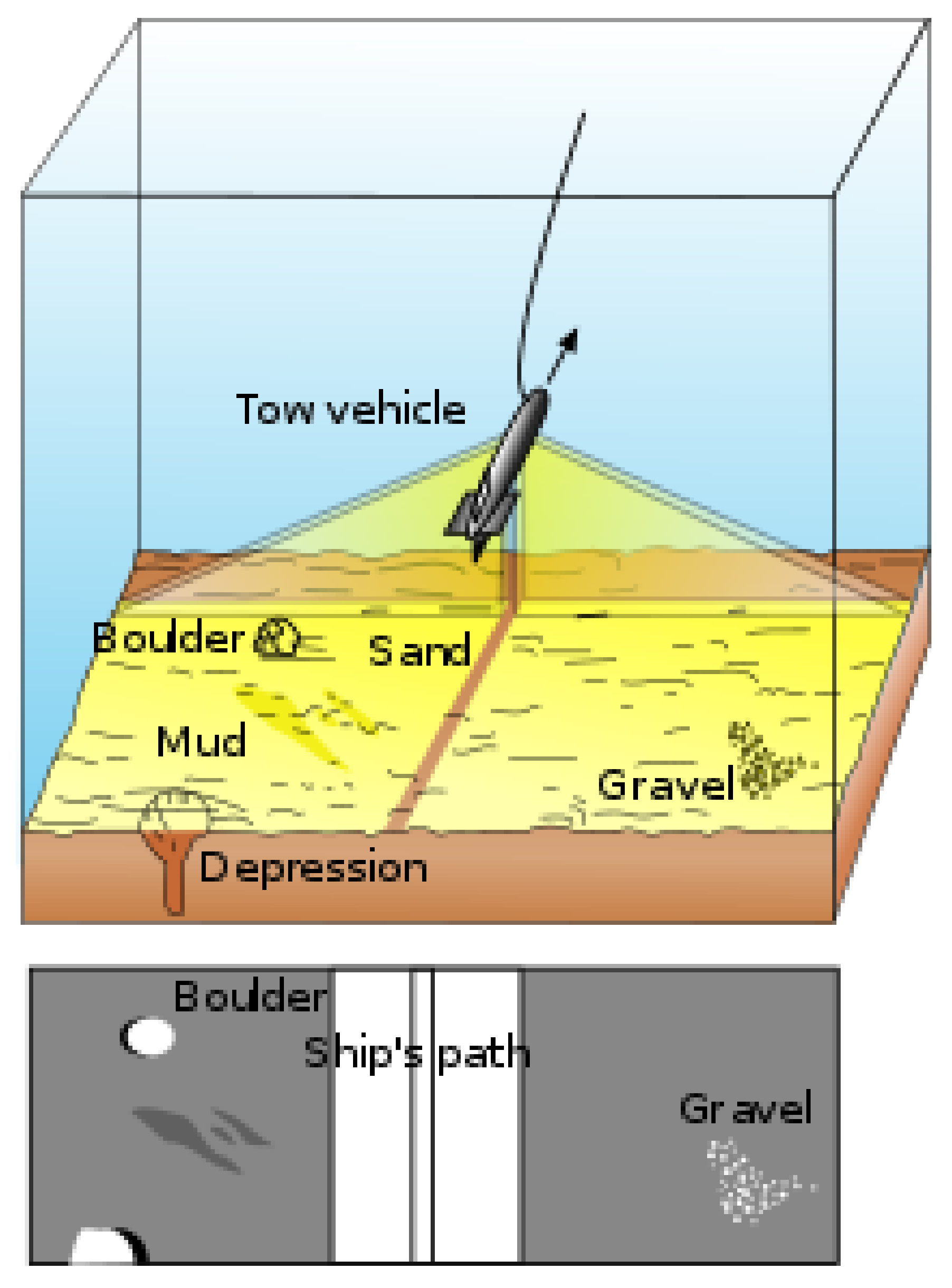
Side-scan sonar systems consist of a dual-channel tow-fish device capable of operating in water depths for the survey and contain a tracking system [1,2]. The device is usually towed from a surface vessel or submarine, or mounted on the ship’s hull (Figure 1).
The device emits conical or fan-shaped pulses down toward the seafloor across a wide angle perpendicular to the path of the sensor through the water. The equipment is used to obtain complete coverage of the specified areas and operates at scales commensurate with line spacing, optimum resolution and 100% data overlap. This coverage is attained by transmitting one beam on each side, broad in the vertical plane and narrow in the horizontal plane (Figure 1). The height of the tow-fish above the seabed and the speed of the vessel are adjusted to ensure full coverage of the survey area. The maximum tow-fish height is 15% of the range setting. The intensity of the acoustic reflections from the seafloor of this fan-shaped beam is recorded in a series of cross-track slices. When stitched together along the direction of motion, these slices form an image of the sea bottom within the coverage width of the beam. This instrument covers a much larger portion of the seabed away from the surveying vessel, from a few tens of meters to 60 km or more.
The track line under the ship carrying the sonar, the acoustic shadow generated by the beam, as well as many other factors (listed below), impair target detection [4].
Side-scan data are frequently acquired along with bathymetric soundings and sub-bottom profiler data, thus providing a glimpse of the shallow structure of the seabed. Today a wide variety of commercial components with excellent capabilities is available on the market for every application.
1.3. Frequencies Used
The sound frequencies used in side-scan sonar usually vary from 100 to 500 kHz. Higher frequencies yield better resolution but smaller range; frequencies from 6.5 kHz to 1 MHz achieve resolutions of 60 m down to 1 cm. A complete list of frequencies used in underwater acoustics can be found in chapter 2 of [1].
Recorder settings are continuously monitored to ensure optimum data quality. Onboard interpretation of all contacts identified during the survey is undertaken by a geophysicist suitably experienced in side-scan sonar interpretation. The processing steps are less standardized, depending on the manufacturer, despite the consensus on the types of corrections desirable [5].
1.4. Side-Scan Sonar Applications
Side-scan sonar imagery is frequently used to detect debris and other obstructions on the seafloor that may be hazardous to navigation or to seafloor installations by the oil and gas industry. A high-precision, dual-frequency side-scan sonar system can obtain seabed information along the routes for example, anchor/trawl board scours, large boulders, debris, bottom sediment changes, and any item on the seabed having a horizontal dimension in excess of 0.5 m [5,6]. Side-scan data are frequently acquired along with bathymetric soundings and sub-bottom profiler data, thus providing a glimpse of the shallow structure of the seabed.
Side-scan sonar is also used for fisheries research, dredging operations, and environmental studies. Multi-frequency, multi-sonar echosounders are used for benthic habitat mapping [7,8].
Side-scan sonar may be used to conduct surveys for maritime archaeology [9]; in conjunction with seafloor samples, it is able to provide an understanding of the differences in material and texture type of the seabed.
1.5. Objective and Paper Organization
This research deals with the problem of the detection of man-made objects detected in side-scan sonar images. Man-made objects tend to have regular shapes which can be identified by obtaining their contour [4]. The most common process for separating an image into regions or their contours corresponding to objects is segmentation. Contours are obtained by identifying differences between regions (edges). Since the simplest property which pixels in a region can share is intensity, the simplest method for image segmentation is thresholding [11,12]. Thresholding is an important technique in image segmentation, enhancement, and object detection. Thresholding creates binary images (pixel values 0 or 1) from grayscale images (pixel values from 0 to 255) by turning all pixels below some threshold to zero (i.e., black) and all pixels above that threshold to one [11,12,13,14].
Histograms show that side-scan sonar images are in general multi-mode images; hence, our target is to compute a proper threshold given the image histogram. The objective of this work is to propose adaptive thresholding methods for contour extraction in side-scan sonar images, confronting shadows and other impairments produced by various causes. The resulting black and white image should contain the outline of the object for further processing such as automatic target recognition, classification, and storage in large-scale multimedia databases.
In order to demonstrate the concepts, two Octave scripts implementing the proposed algorithms have been developed, one for each method. The scripts have 430 and 400 lines of code respectively and are also compatible with MATLAB (with the exception of the Octave data smoothing functions).
This paper is organized as follows: Section 2 presents related work and common problems in SSS research; Section 3 presents the research results obtained by conventional methods. In Section 4 the proposed algorithm is presented. Section 5 presents the results of the proposed methods using a case study. A discussion follows in (Section 6). Finally, Section 7 concludes the paper.
2. Literature Review and Reseach Problems
2.1. Related Work
Several algorithmic techniques for image thresholding have been presented in the literature. Otsu’s optimal thresholding technique [11,12,15] calculates a global threshold value. It starts by computing the gray-level histogram of an image and then the global threshold is determined by minimizing the so-called within-class variance of the thresholded black and white pixels. It works well with images having uniform distribution of black background and white foreground pixels. It essentially maximizes the weighted distances between the global mean of the image histogram and the means of the background and foreground intensity pixels. Several improvements of the Otsu’s technique have been proposed in the bibliography [16]. An improvement of Otsu’s threshold segmentation technique for underwater application with simultaneous localization and mapping-based navigation is presented in [17]. Otsu’s method for automatic image thresholding is implemented by the function graythresh.m in MATLAB [11,18] and Octave [19].
Gonzalez and Wood’s technique [11,13,20] also finds a global threshold value. It starts by selecting an initial threshold value T between the minimum and maximum intensity values in the image. Then using this T value, the image is segmented into two groups to produce pixels in group G1 with intensity values greater than or equal to T, and pixels in group G2 with intensity values less than T. Next it computes the mean intensity values 1 in group G1 and 2 in group G2; the new threshold value is calculated as the average between the two mean values, i.e., . This procedure continues recursively until the difference in T in successive iterations is smaller than a predefined value .
Singh and co-researchers [21] devised a locally adaptive thresholding technique to accommodate degraded document images without uniform distribution of background and foreground pixels. Their technique uses local mean and mean deviation to remove the background pixels. The local mean computation is independent of the window size and uses the integral sum image for pre-processing; as a result the authors claim that their technique is faster compared to other local thresholding techniques.
Arora and co-researchers [22] proposed an algorithm to determine an optimum number of thresholds to segment an image using mean and variance values for each segment. The optimum number of thresholds is determined by utilizing the Peak Signal to Noise Ratio (PSNR) of the original and segmented images, as the rate of increase in the PSNR decreases with the number of thresholds n and tends to saturate. After determining the optimum number of thresholds, the algorithm, starting from the values at both ends of the original histogram plot, is applied recursively on sub-ranges computed from the previous step, so as to find a threshold value and a new sub-range for the next step, until no significant improvement on image quality is achieved.
Chang and Wang [23] use a lowpass/highpass filter repeatedly to adjust (decrease/ increase) the number of peaks or valleys to a desired number of classes and then the valleys in the filtered histogram are used as thresholds. Unfortunately, many thresholding algorithms are not able to automatically determine the required number of thresholds, as has been noted by Whatmough [24].
2.2. Problems in Side-Scan Sonar Research
The problems investigated in side-scan research fall into one of the following categories:
2.2.1. Sound Problems
- 1.
- Signal degeneration in the ocean is due to:
- (a)
- refraction of sound;
- (b)
- attenuation of sound;
- (c)
- reflection from surface and bottom and Lloyd mirror effect;
- (d)
- signal fluctuation.
- 2.
- Scattering of sound in the ocean is due to [29]:
- (a)
- dependence on the properties of the sound source;
- (b)
- dependence on time;
- (c)
- distribution of the scatterers in the ocean;
- (d)
- frequency and coherence characteristics of the scattered sound.
Especially the single transmitter/single receiver systems face two common problems:- (a)
- the system response is range variant;
- (b)
- the range curvature effect also called range migration [10].
- 3.
- 4.
- The interference of the returned echoes, due to multiple reflections, each with different received frequency and power, fades and distorts the signal.
2.2.2. Illumination Problems
2.2.3. Other Problems
- 1.
- Camera jitter. In real surveillance applications, the camera itself moves frequently. Hence, the pixel correspondence between the background and the image changes frequently [31] resulting in artifacts appearing as extra noise.
- 2.
- Rapid changes in temperature (thermocline zone) or salinity (halocline zone) or the presence of strong chemical gradients (chemocline zone) reduce the scan range and distort the image. These phenomena take place below the surface zone (typically, at depths of 1000 m or more) [32].
- 3.
- Ocean instabilities like waves, water currents, wind, etc. [10].
3. Contour Extraction Using Conventional Methods
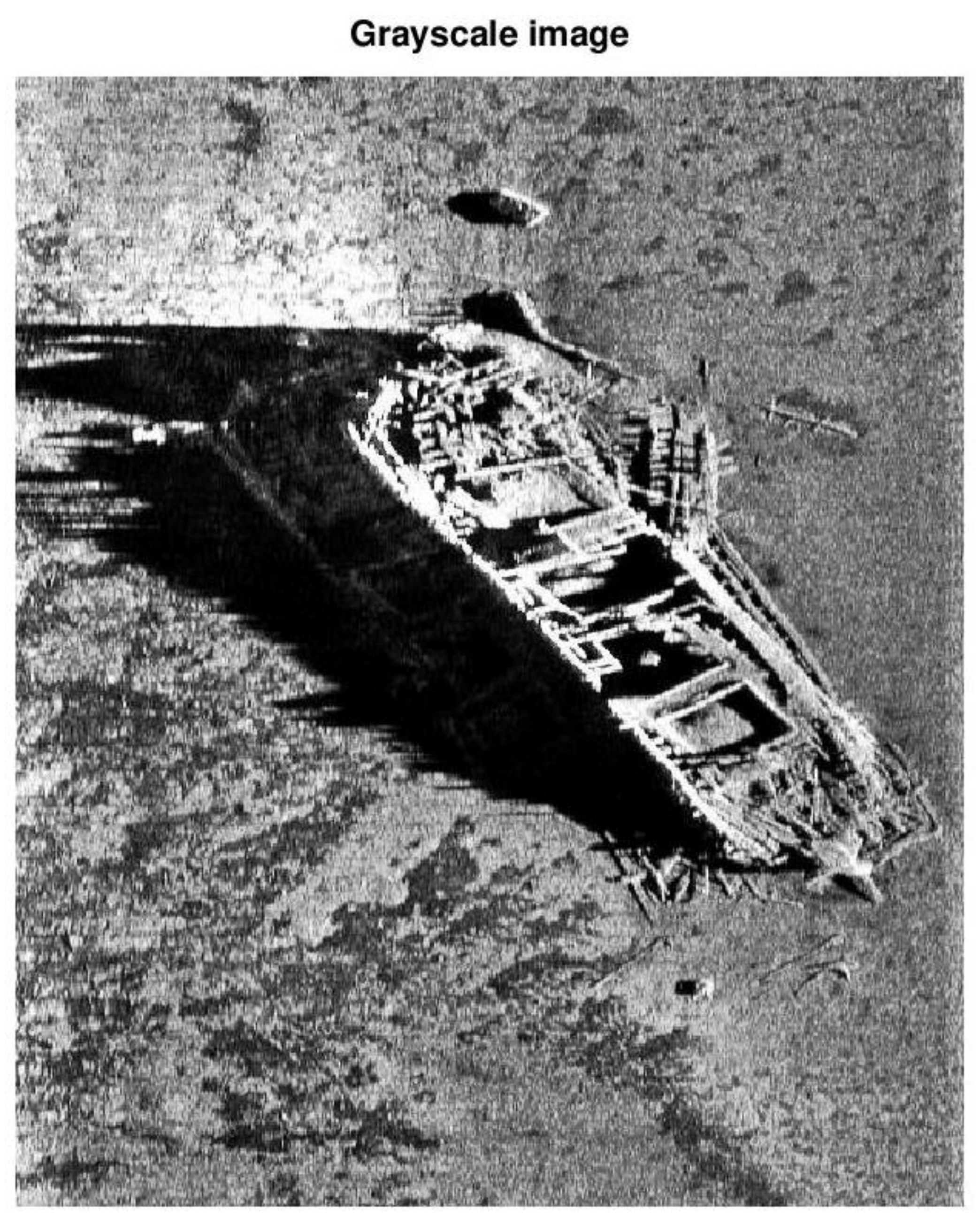
In this section, we delve into the problem of contour extraction using conventional methods. As we shall see, the conventional methods produce poor contours because they cannot successfully remove hard shadows and other artifacts which impair side-scan sonar images. In this research, we consider 8-bit, 2D grayscale images. Hence, the pixel values range from 0 to 255, with 0 representing absolute black and 255 representing absolute white. For binary images, the pixels can be 0 or 1.
The test image of our case study is shown in Figure 2. An ideal contour extraction method is expected to eliminate the acoustic shadow (black area), mask excessive light (white pixels at top left), filter the background noise, and keep only the ship contour (as white on a black background).
3.1. Using Popular Thresholding Methods
In this subsection, the performance of popular legacy thresholding methods such as Otsu’s and Gonzalez–Woods’ thresholding algorithms will be presented.
To implemented Otsu’s method we first use the function ‘graythresh’ to compute a global threshold from the grayscale image; next we use this threshold to convert the grayscale image to binary using function ‘im2bw’ [11,19]. The result produced by Otsu’s method is shown in Figure 3. As we can see, the result is unsatisfactory because shadows remain and the background noise is not eliminated.
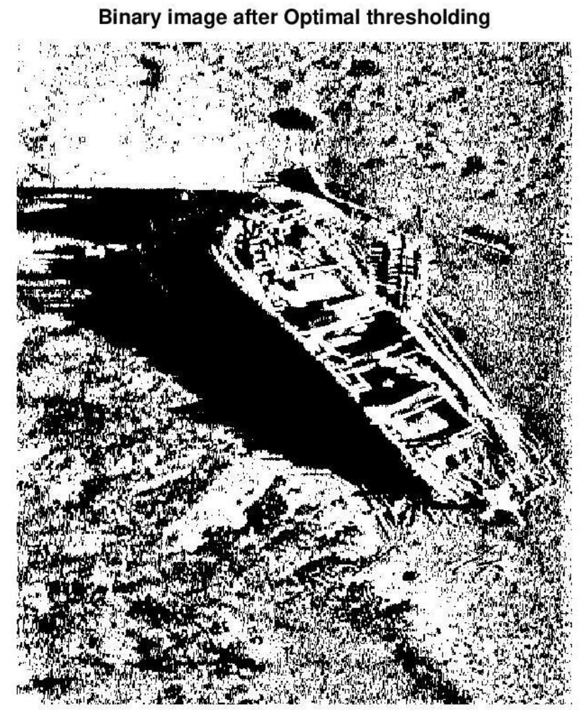
Optimal threshold is computed by the function ‘opthr’ [19]. Optimal thresholding also fails for the same reasons (Figure 4).
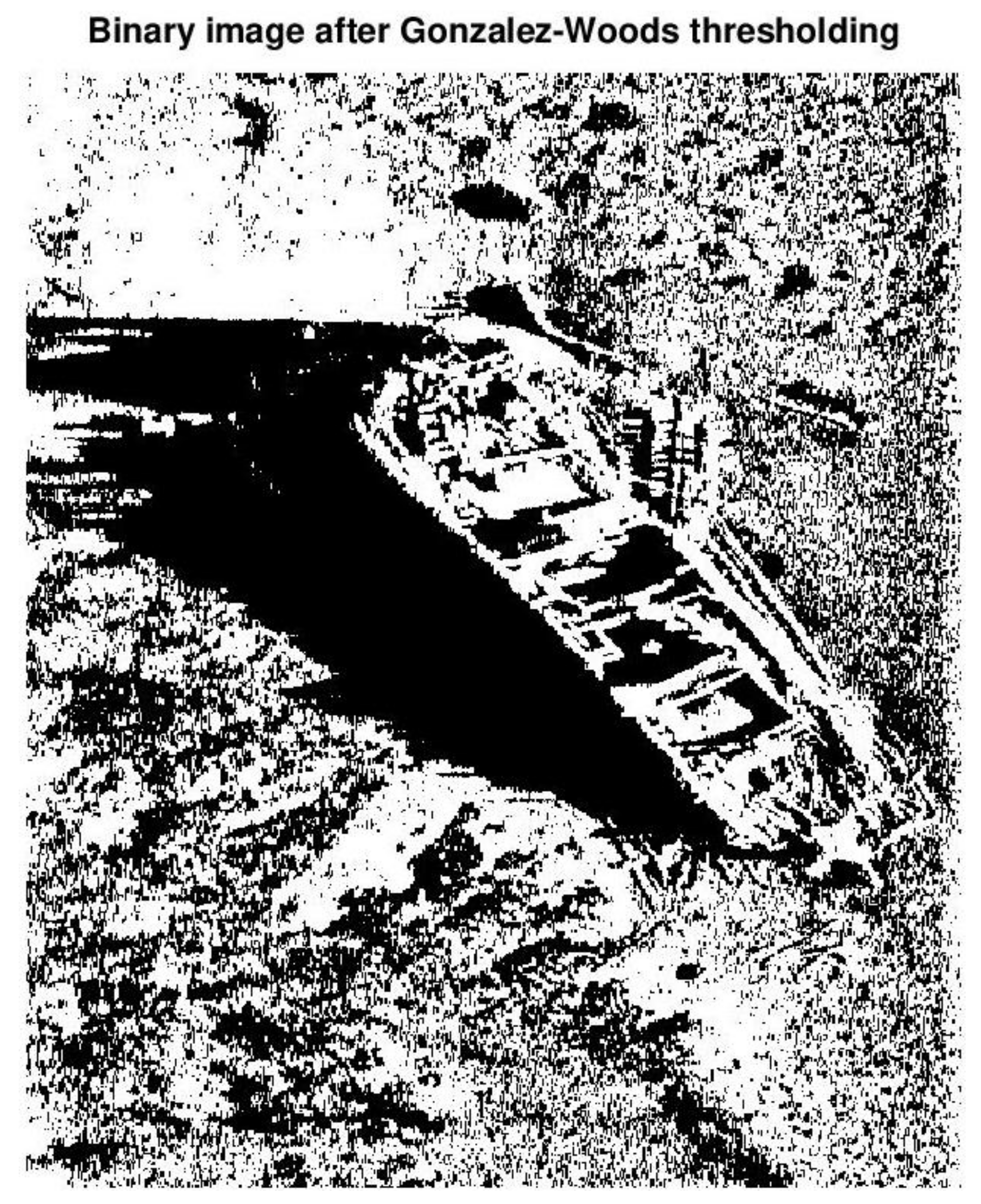
The Gonzalez–Woods method is implemented by code adapted from [11]. The produced result is shown in Figure 5 and is not satisfactory as well.
In conclusion, popular legacy thresholding methods produce comparable results. All of them fail to highlight the target because they are not intended to separate specific objects (or modes) from the images, but instead, they treat all objects in the same manner.
3.2. Using Edge Detection Filters
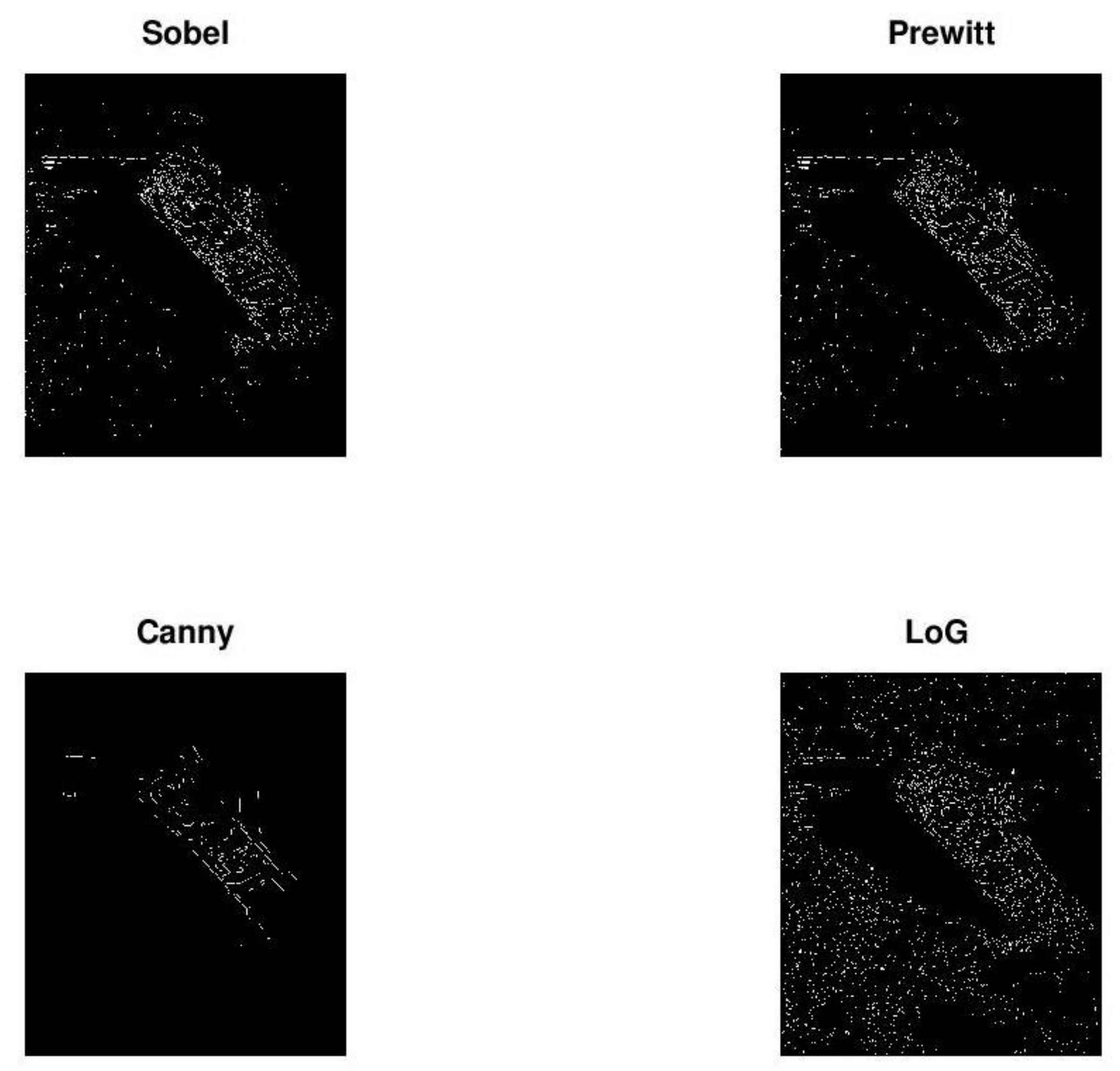
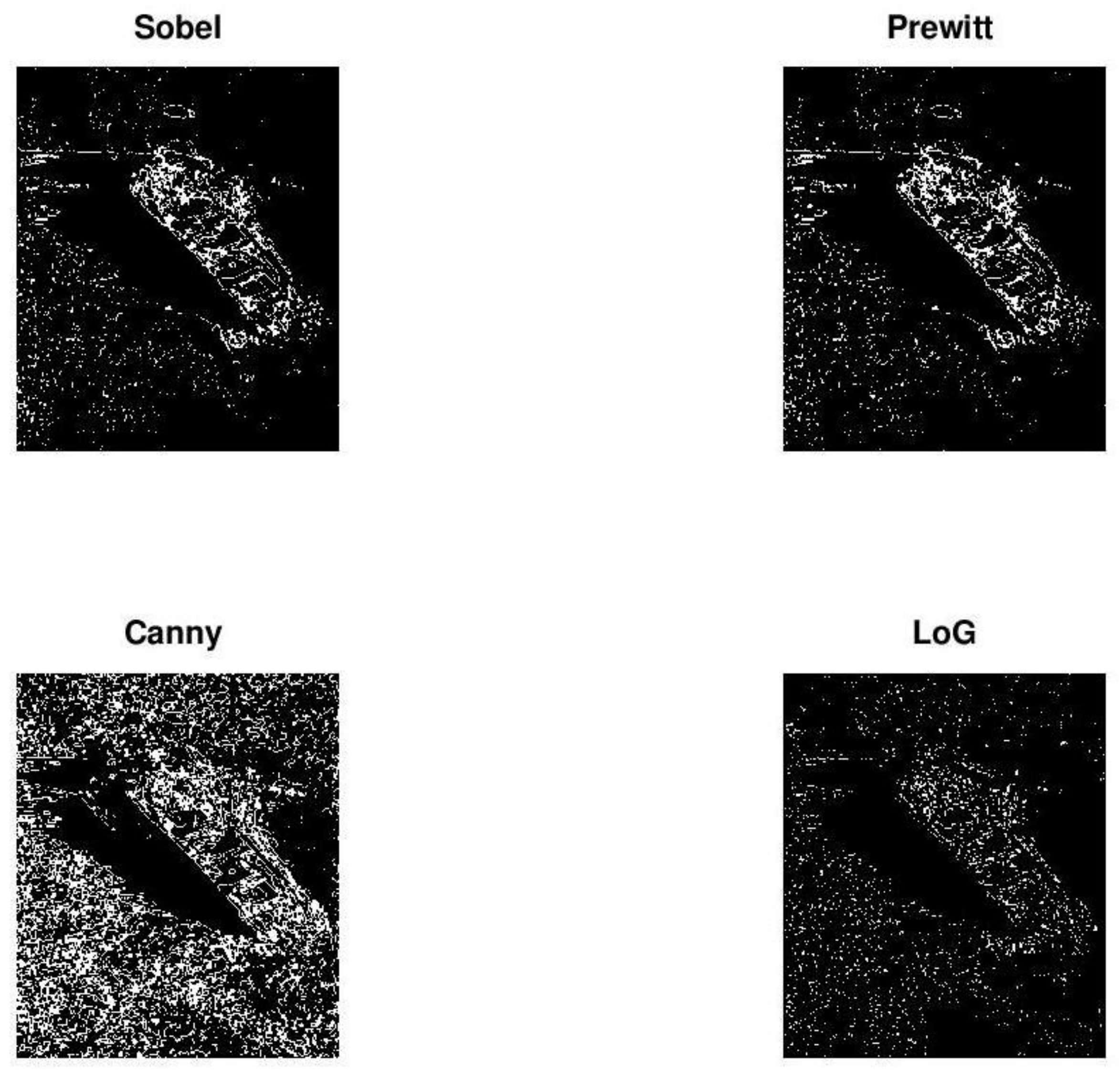
A common method for contour extraction is edge detection [11,12]. Common edge-detection algorithms have been proposed by Roberts (1965), Prewitt and Mendelsohn (1966), Sobel (1970), and Canny (1986) [12], and have been implemented in MATLAB Image Processing Toolbox [18], as well as Octave and its image package [19].
Figure 6 presents the result of four common edge detection filters with default parameters, namely: Sobel, Prewitt, Canny, and Laplacian of Gaussian (LoG). As we can see, none of these common edge detection filters produces satisfactory results.
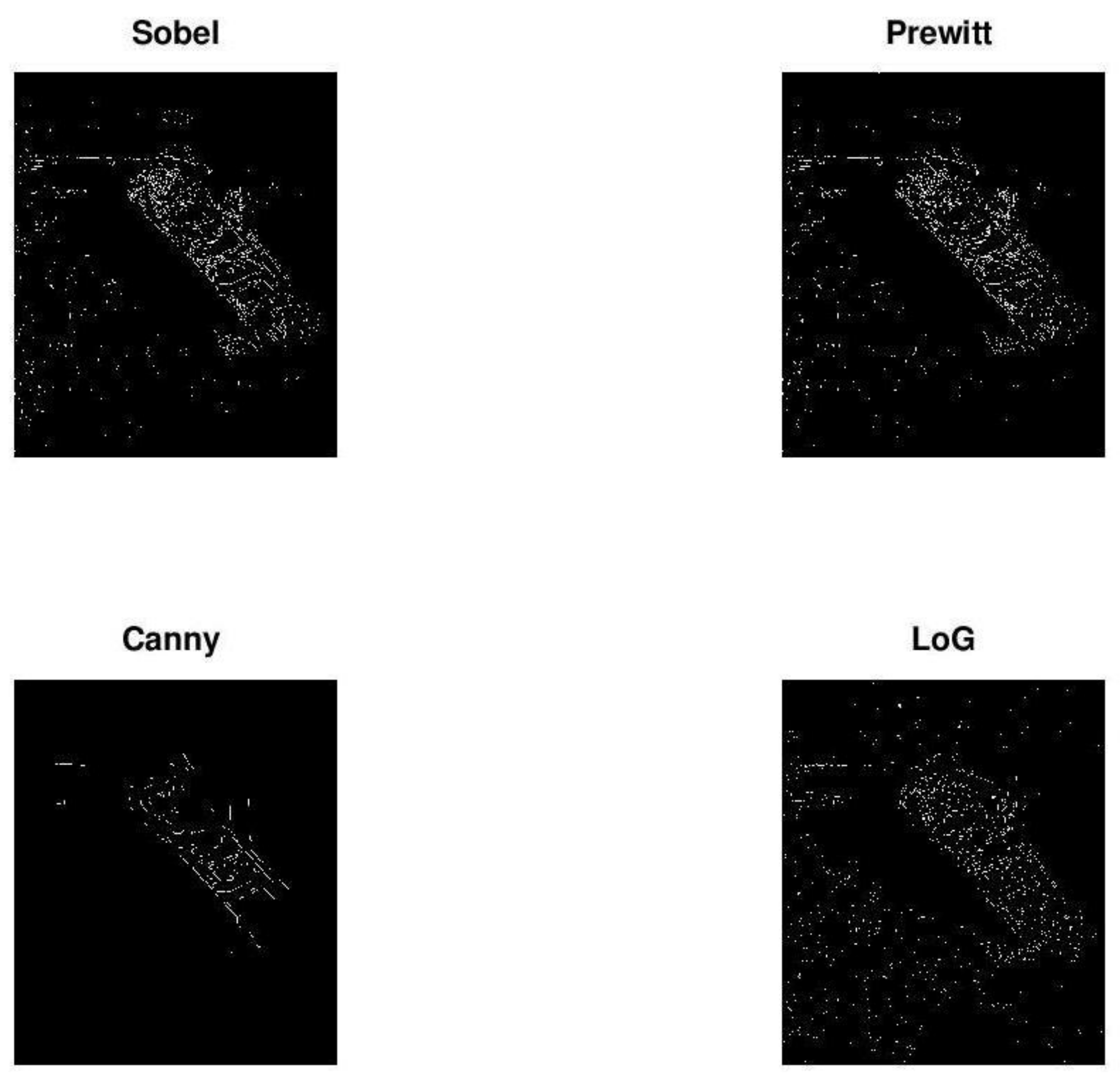
The result may be partially improved if we use filter parameters different from the default values (but the concept is to design an algorithm that works automatically, i.e., without any interventions). After experimentation, we got the results presented in Figure 7.
The background noise has been largely removed but the shape of the boat is unclear because the lines are thin and discontinuous. Another disadvantage is that the proper filter parameters must be chosen experimentally for each particular image.
3.3. Using Morphological Transformations
Morphological image processing consists of a set of operators which transform images using mathematical morphology [11,12,33]. The basic morphological operators are erosion, dilation, opening, and closing. The fundamental operations are erosion and dilation; opening is the dilation of the erosion of an image while closing is the erosion of the dilation of that image, also referred to as ‘corrosion expansion’ [34]. Octave and MATLAB support morphological operations with several functions of their image processing libraries [19,35].
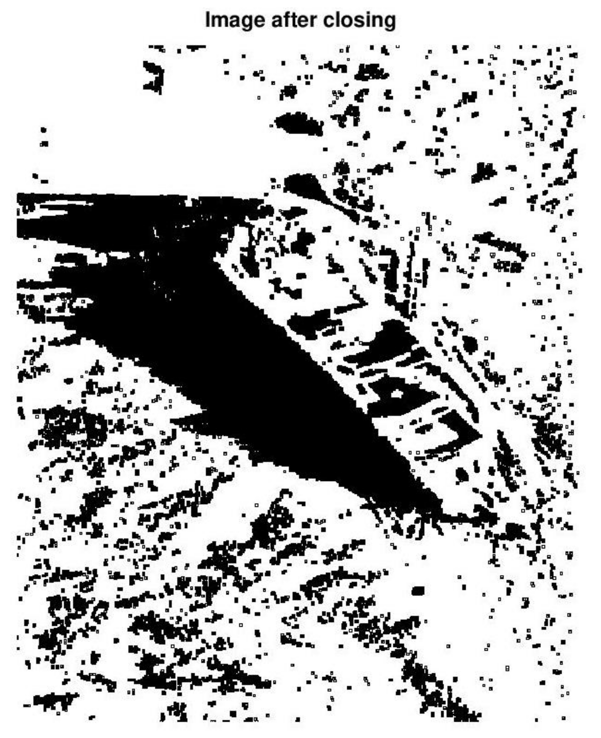
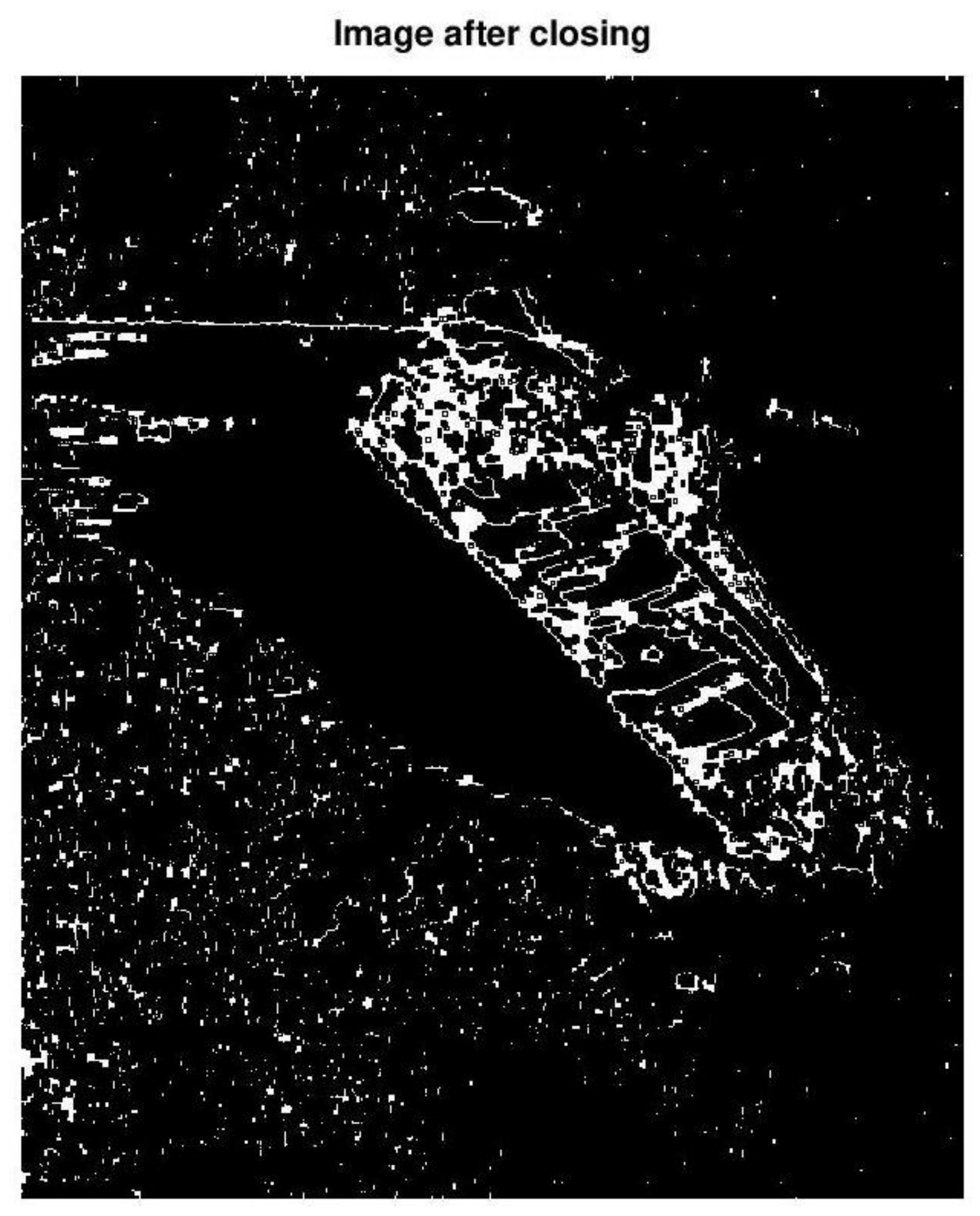
Figure 8 presents the result of corrosion expansion (closing) for the binary image obtained after Otsu thresholding. The result is bad because the shadow and the background noise remain, so the object contour is not clear. Figure 9 presents the result of the corrosion expansion algorithm of the Kirsch edge detection filter [11,19]. There is some improvement but still, the target is not clear while much of the noise remains.
4. Methodology—Proposed Solution
4.1. The Concept
In practice, side-scan sonar images are multimodal [15] (the modes being non-Gaussian); hard shadows form a black mode (peak) on the left of the histogram, object edges (along with noise in some cases) form another mode on the right of the histogram, and the background (possibly with part of the object) form a central (gray) mode in the middle of the histogram. Hence, the problem of calculating the optimal threshold reduces to finding the valley between two overlapping peaks (modes) representing the background (gray pixels) and the object contour (almost white pixels).
In the grayscale image, the contour of the objects is white, hard shadows are black and the background is gray, roughly. An ideal thresholding algorithm should isolate the contour, in other words, the whitest (rightmost) mode. Therefore, the proposed algorithm places the threshold at the valley just before the rightmost mode of the histogram and uses this threshold in order to convert the grayscale image into a binary image.
4.2. Locating Peaks and Valleys
A simple way to calculate a suitable threshold is to find the local maxima (corresponding to modes) and the local minima (valleys) between them. While this method appears simple, there are two problems to be solved:
- 1.
- The sum of two or more separate non-Gaussian distributions, each with their own mode, may not produce a distribution with distinct modes.
- 2.
- The histogram is very rough (unsmooth), containing many local minima and maxima. To get around this, the histogram should be smoothed before trying to isolate the separate modes.
To overcome the above problems we propose the following two alternatives:
4.3. The Process
A proper algorithm should filter out the background noise and the acoustic shadow, keeping only the contour of the objects. In addition, it should emphasize the contour, a process that improves the result when the contour is very thin or discontinuous.
In the proposed algorithm, contour extraction is based on automatically estimating the optimal threshold for converting the original grayscale image into binary.
The algorithm steps are outlined in Table 1.
Analytically the steps are as follows:
- 1.
- Input the grayscale SSS image to process.
- 2.
- The histogram of the original grayscale image is computed.
- 3.
- Calculate the envelope of the histogram.
- 4.
- The envelope of the histogram is approximated by two methods. In method 1 we use polynomial curve fitting. This process resolves noisy histograms resulting in few maxima and minima. In method 2, data smoothing algorithms produce a smooth curve from the envelope of the histogram.
- 5.
- The maxima and minima of the above curves are calculated. The abscissas (x-values) of peaks and valleys are then computed.
- 6.
- The optimal threshold is the valley before the rightmost peak (mode) of the histogram.
- 7.
- Convert the grayscale SSS image into a binary image using the optimal threshold. Experimentally, it turns out that the optimal threshold value produces few white pixels (2–5%) which represent the foreground object (not just its edges) and filters out the background noise and hard shadows.
5. Results
In this section a step by step demonstration of the procedure will be presented. The test image of Figure 2 will be used.
5.1. Method 1: Curve Fitting
Figure 11 presents the histogram of the test image. As we can see, this is a tri-modal histogram; the proposed algorithm places the threshold just before the rightmost peak, between x = 200 and x = 250.
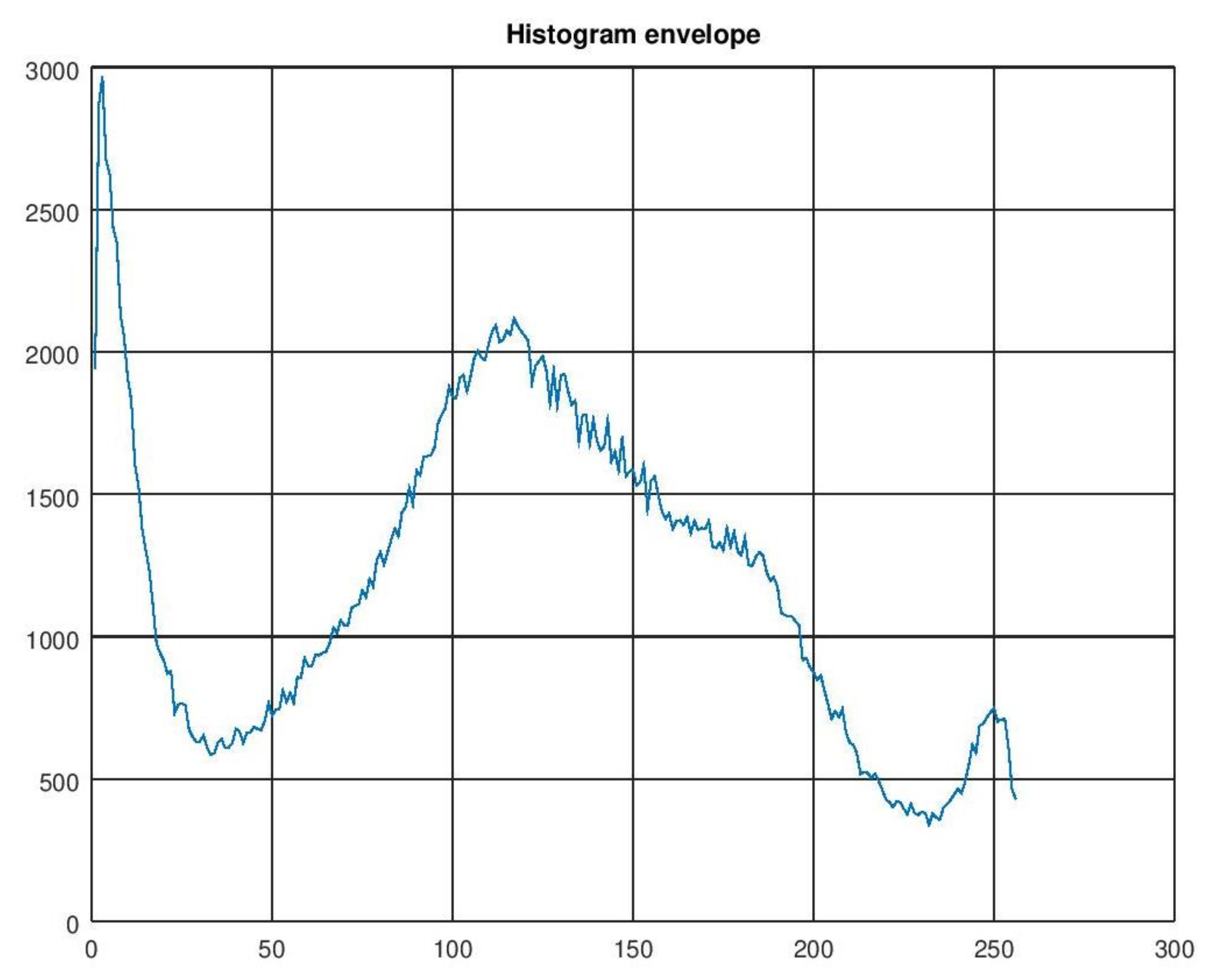
Figure 12 presents the envelope of the histogram. The result is not satisfactory because it contains many local minima and maxima.
Next, polyfit and polyval functions are used to approximate the envelope with a polynomial of degree n = 6. Figure 13 presents the envelope of the histogram and the curve of the fitting polynomial.
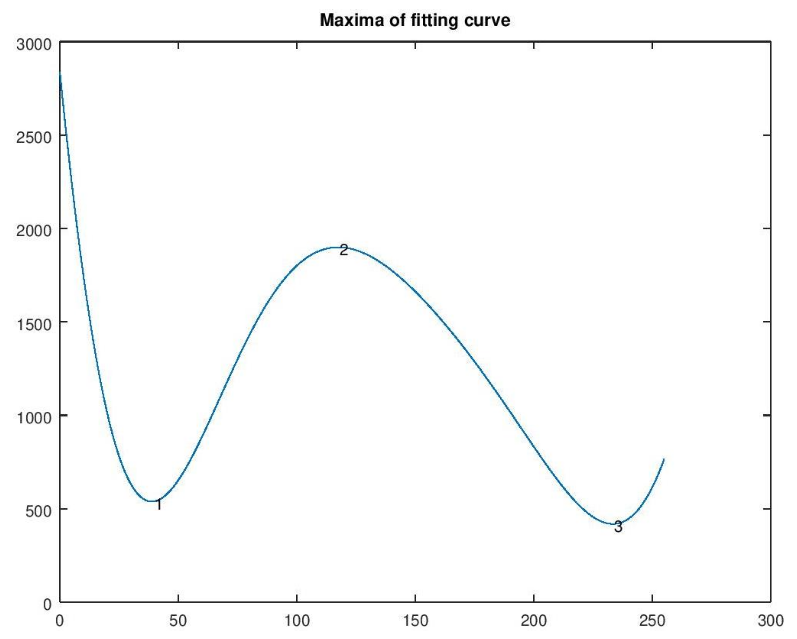
Figure 14 presents local maxima and minima. The maximum of the polynomial curve corresponding to the central mode is numbered 2. The peak is at x = 118. It also presents the minima (numbered 1 and 3). The valleys are at x = 40 and 234. Valley at x = 234 satisfies our requirements and produces the result shown in Figure 15 which is satisfactory.
5.2. Method 2: Data Smoothing
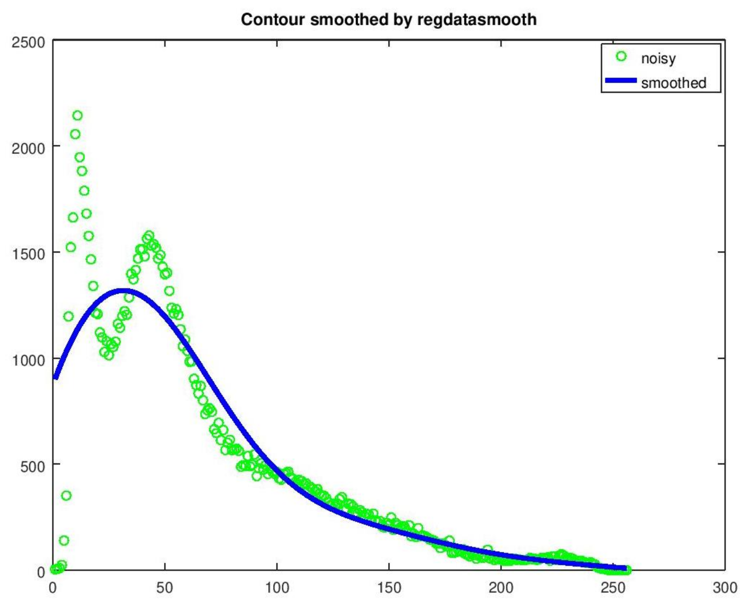
The algorithm follows the same steps presented in Table 1 but differs in step 4: method 2 uses data smoothing. A special library such as Octave Data smoothing package [42] will be used. Two functions from this package were used: (a) regdatasmooth [40]; (b) rgdtsmcore [41].
Regdatasmooth smooths the y vs. x values of the histogram envelope by Tikhonov regularization. Regdatasmooth is the recommended function because it can be used directly and has more features. This function also returns the regularization parameter lambda that was used for the smoothing. Rgdtsmcore also smooths y vs. x values by Tikhonov regularization. It needs lambda as an input variable [42].
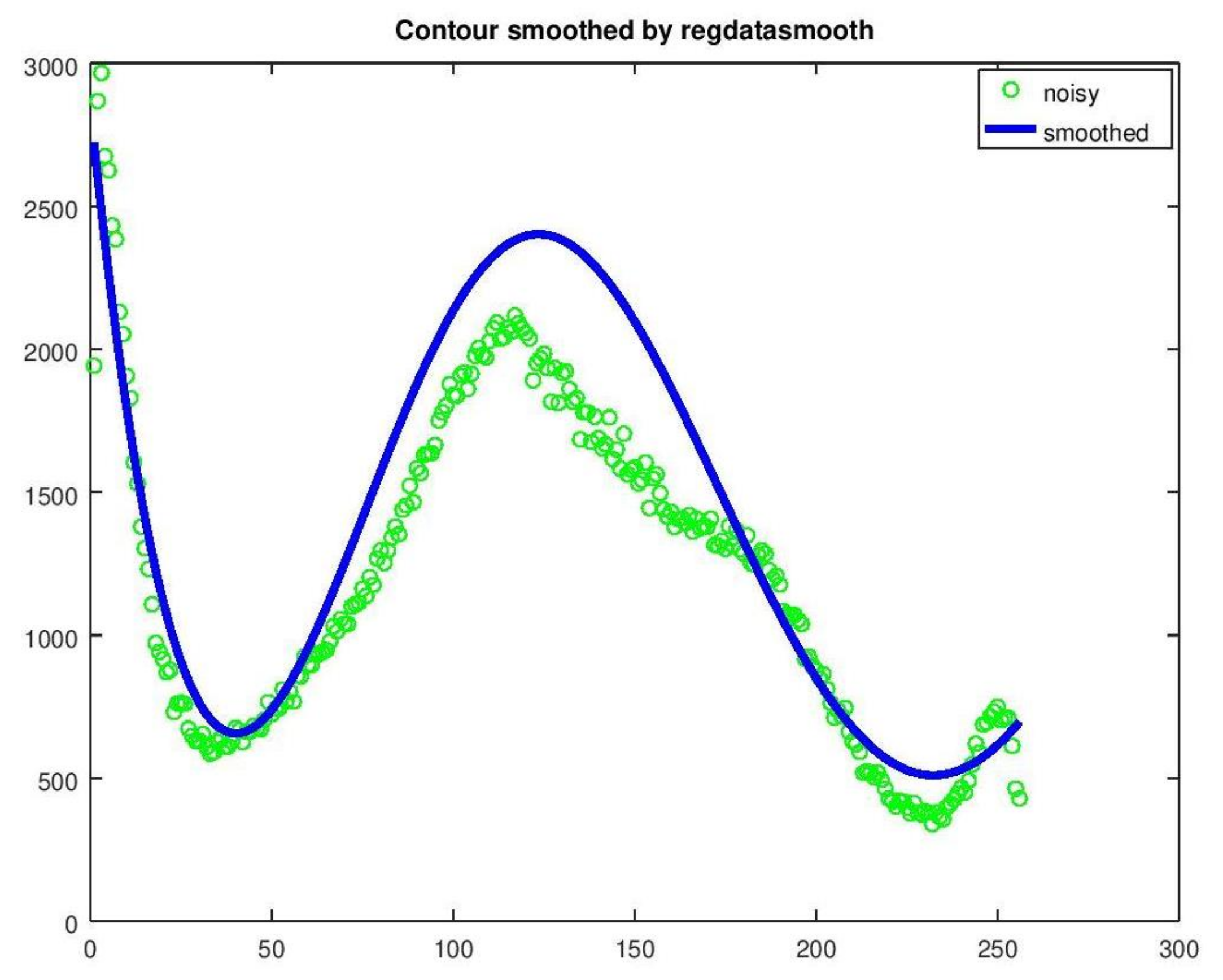
Figure 16 presents the data-smoothing curve produced by regdatasmooth. The fit is worse than that of method 1 but the value of the local minimum (i.e., the threshold) is correct (x = 232) and very close to that of method 1 (x = 234).
Figure 17 presents the resulting image produced by regdatasmooth and is comparable to that of method 1 (Figure 15).
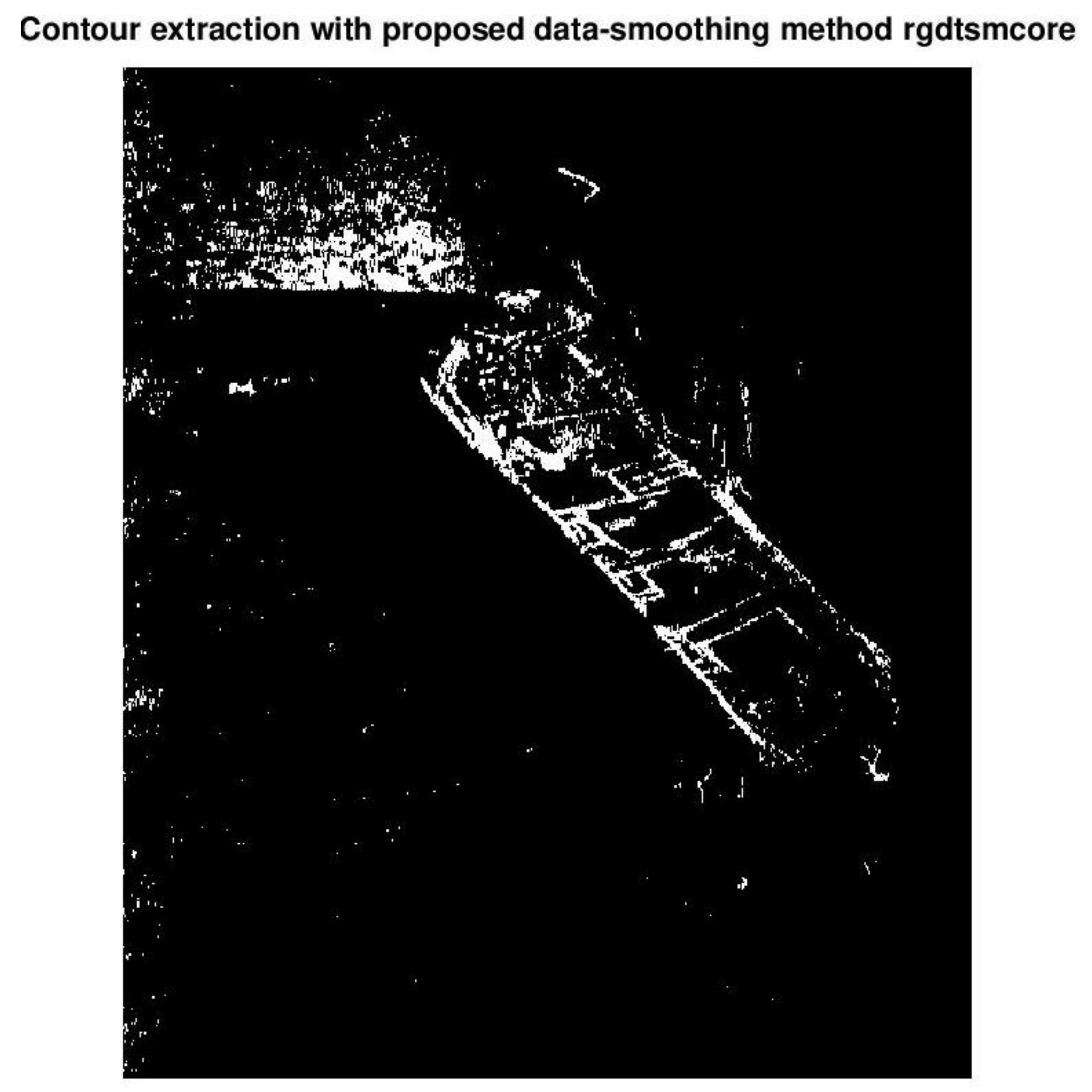
Figure 18 presents the data-smoothing achieved by rgdtsmcore. Again the fit is worse than that of method 1 but the calculated threshold (x = 236) is correct and very close to that of method 1 (x = 234).
Figure 19 presents the resulting image produced by rgdtsmcore.
5.3. Comparison with Other Methods
The thresholds computed by methods 1 and 2 are shown in Table 2. On the second row there is the computed threshold in the range (0, 255) while on the third row there is the normalized threshold in the range (0, 1). Clearly, the thresholds computed by our algorithm are close to each other and far from those computed by legacy thresholding methods.
5.4. Further Contour Enhancement
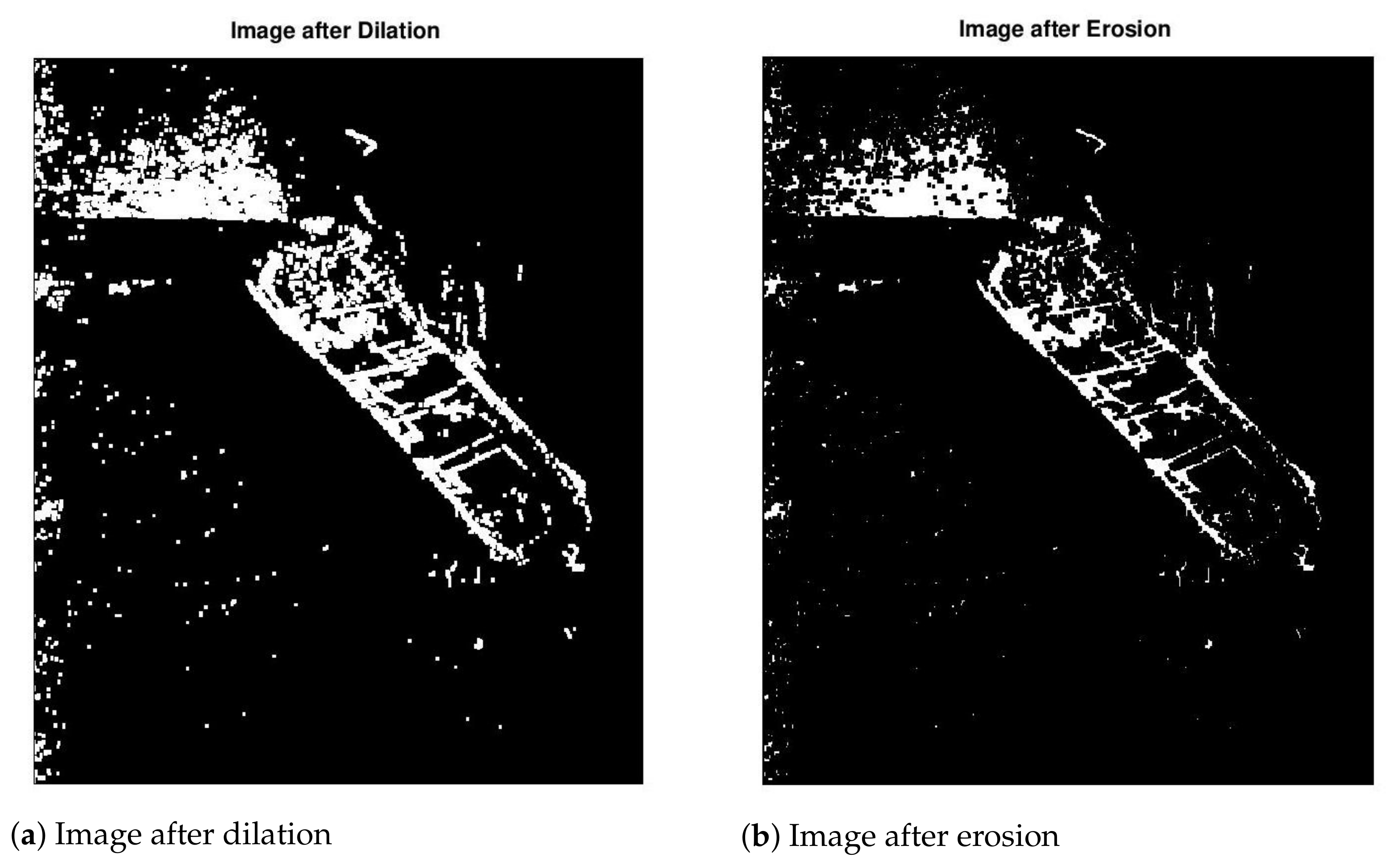
A further enhancement is possible when the detected object contour is thin. Morphological transformations can be used to improve the contour of the target [11,12,33]. Figure 20 demonstrates the result of corrosion expansion for our test image, implemented as erosion of the dilation of the outcome of our method 1. Dilation highlights the target but also the white background noise (top left). Erosion suppresses the background noise but makes the target contour thinner.
5.5. Other Test Images
In this subsection concise results obtained by method 1 for the following test images are presented: Frank Palmer, shipwreck world, boat, Florida’s treasure coast, and bike. Each of these images represents a particular case but the proposed algorithm produces satisfactory results in all cases. The results obtained by method 2 are similar and are omitted for reasons of brevity.
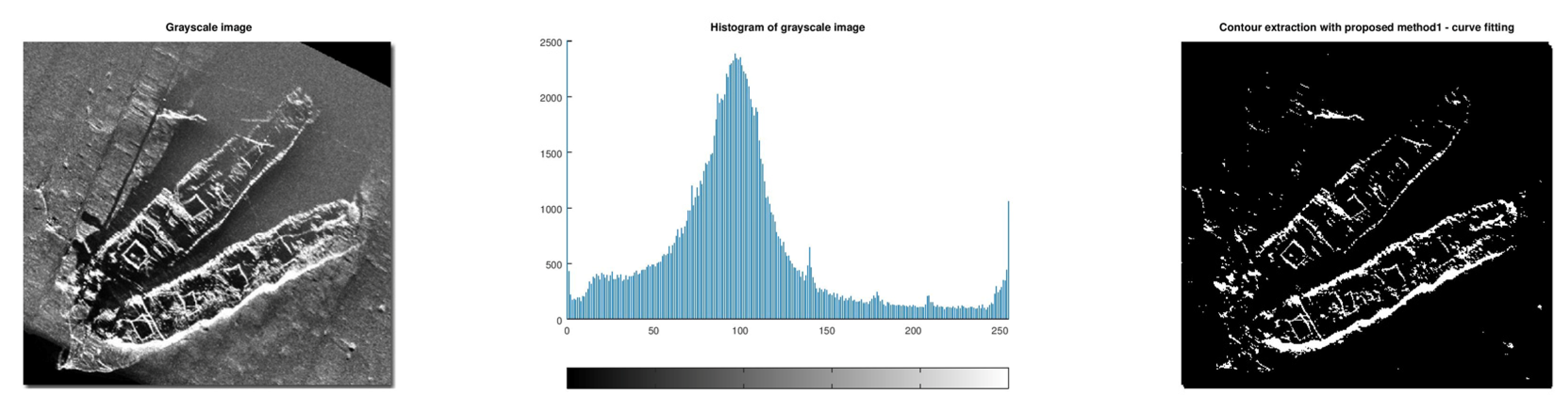
5.5.1. Test Image Frank Palmer
The challenges in this test image are to separate the object from the background and to filter out the black triangles (top right and bottom left) which correspond to areas not covered by the side-scan sonar beam. Additional artifacts due to several problems explained in Subsection 2.2 also exist (Figure 21).
5.5.2. Test image Shipwreck World
The challenge of this test image is the shadows and the varying illumination (Figure 22).
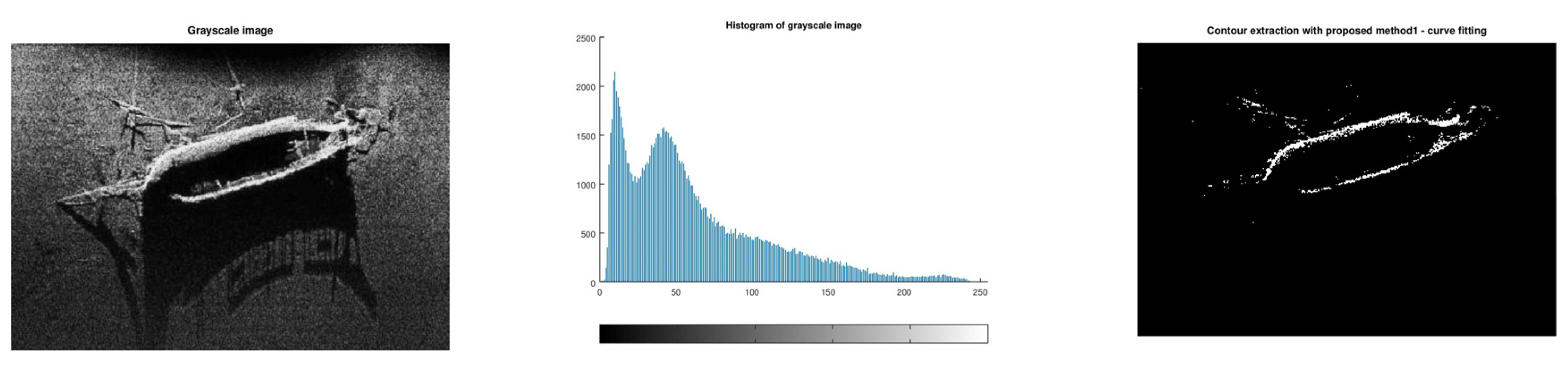
5.5.3. Test Image Boat
The problem in the test image boat is the hard shadows inside and outside the boat (Figure 23).
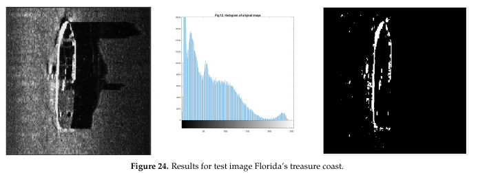
5.5.4. Test Image Florida’s Treasure Coast
The problems in test image Florida’s Treasure Coast are the low resolution and the hard shadow (Figure 24).
5.5.5. Test Image Bike
The proposed method works also on “tough” images such as bike, with a noisy, poor quality histogram—when all other methods fail (Figure 25).
6. Discussion
In this paper we have presented a novel algorithm that improves contour extraction in SSS images. Our results can be useful in applications searching for man-made objects on the seafloor such as maritime archaeology, shipwreck detection, military applications, and underwater development.
It is obvious that the performance of the proposed methods depends on the quality of the input images. Clearly, poor-quality images will produce poor results. In Section 2.2 we have presented a set of causes degrading image quality. Poor-quality images have poor resolution, poor ensonification, noise, jitter, artifacts, etc.
6.1. Performance of Method 1
The performance of method 1 (curve-fitting) is affected by the degree of the fitting polynomial, n. In our experiments we have successfully tested polynomial degrees from n = 4 to n = 20; n = 6 works fine with all test images. The reason is that typically tri-modal SSS image histograms have three peaks and three (or two) valleys (see Figure 11 and Figure 21, Figure 22, Figure 23, Figure 24 and Figure 25). Intuitively, they can be approximated by a polynomial of degree n = 6. In other words, n = 6 produces a curve flexible enough to fit nicely to tri-modal histograms. Degrees lower than 4 fail to faithfully follow the histogram envelope and may sometimes miss the local minima just before the rightmost mode. Such a case is demonstrated in Figure 26 for the test image boat with n = 3.
A different problem occurs when a low degree polynomial produces a threshold very close to the end of the histogram (x = 255), which results in poor contour extraction. Such a case is demonstrated in Figure 27 for test image shipwreck world with n = 5.
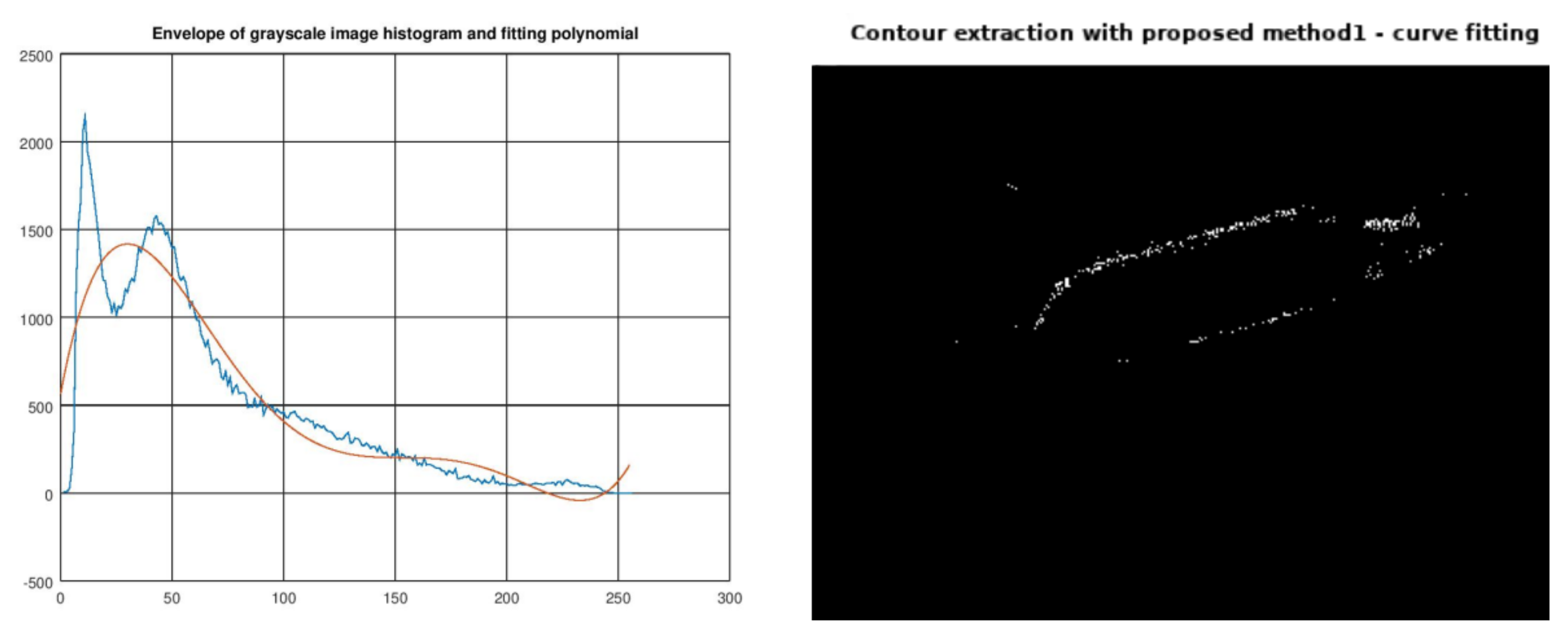
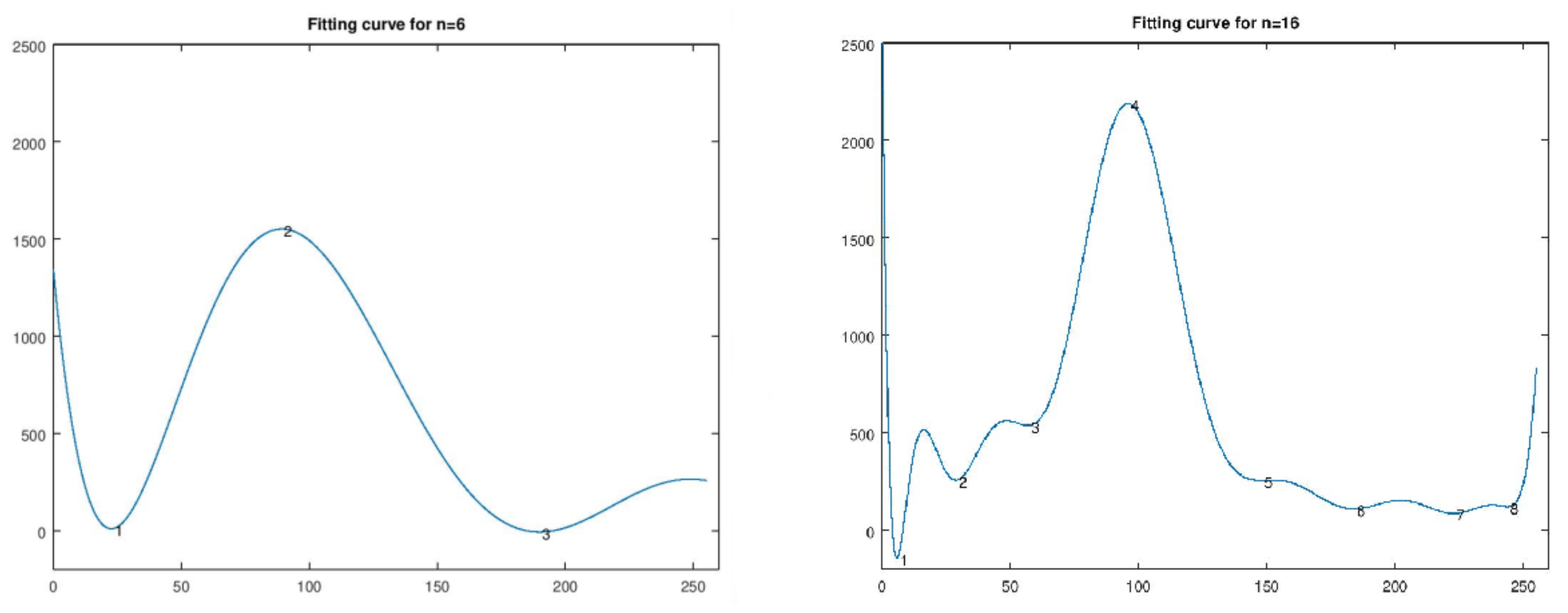
On the other hand, high degree polynomials (such as n = 10 or 16) can achieve a better fit, but produce waveforms with a lot of fluctuation (overfitting). This results in multiple local minima (valleys), raising the problem of optimal valley selection. Valleys with small x values (e.g., around x = 180) fail to eliminate background noise, while valleys with large x values (close to x = 255) produce nearly black images. The latter case is demonstrated in Figure 28 for test image Frank Palmer. On the left we see the fitting polynomial of degree n = 6; on the right, the fitting polynomial of degree n = 16 which produces multiple valleys. The final valley produces a poor result (thin contour). Therefore, high degrees should be avoided.
Method 1 does not perform well when there are very few white pixels, in which case the 3rd mode (target) is under-illuminated.
6.2. Performance of Method 2
The performance of method 2 (data smoothing) in its current implementation is very sensitive to the parameters of the data smoothing functions. Improper selection of parameters may lead the smoothing algorithm to miss the rightmost mode. This case is demonstrated in Figure 29 for the test image shipwreck world. These problems indicate that settings for a particular set of images should be carefully selected.
6.3. Comparison of the Proposed Methods
Our experiments demonstrated that method 1 always managed to produce satisfactory results with polynomial degree n = 6 while method 2 with the specific functions had to be slightly adjusted in a few cases.
6.4. Limitations of the Proposed Algorithm and Future Research
In this research we experimented mostly with SSS images that create tri-modal histograms and found out that method 1 produces satisfactory results with polynomials of degree n=6. But what about histograms with two, four or more modes? It is most likely that the polynomial degree will have to be adapted to the number of modes, so this is an open research problem. In this case, we would like to make our algorithm adaptable to the number of modes: in method 1 by automatically selecting the polynomial degree, while in method 2 by automatically selecting the parameters of the data smoothing functions. We would also like to explore additional data smoothing algorithms.
7. Conclusions
This paper presents an algorithm for contour extraction based on automatically estimating the optimal threshold for converting SSS grayscale images into binary. Simulation results obtained in Octave and MATLAB indicate that the proposed methods produce superior results compared to popular thresholding methods (such as Otsu’s and Gonzalez’s global thresholding) and common edge detection filters (namely Sobel, Prewitt, Canny, and Laplacian of Gaussian), even after corrosion expansion. Moreover, the proposed algorithm is simple, robust, and adaptive.
The algorithm accepts grayscale images as input. The concept is based on the fact that SSS images are multimodal images and hence, seeks to isolate the rightmost mode which corresponds to the target. The algorithm was tested on ten test images. The steps of the algorithm are outlined in Table 1. In step 4, two different methods for finding the optimal threshold, namely curve-fitting and data smoothing were demonstrated. Further improvement is possible by means of morphological operations.
The proposed algorithm manages to extract the contour of man-made objects detected in side-scan sonar images, by selecting a proper threshold that filters out the gray background and eliminates shadows and other impairments, leaving only the object contour after the conversion to black and white.
The two proposed methods could be used in conjunction to enhance accuracy and reliability. The optimal threshold calculated by our methods may be used to guide parametric popular edge-detection filters towards the best results. The resulting black and white images can feed a target recognition system which could apply machine learning methods in order to automatically classify the objects [4,43,44].
The produced black and white images highlight the target contour masking several impairments and reduce the volume of storage needed; hence, they can facilitate automatic target recognition, as well as classification and storage in large-scale multimedia databases.
Author Contributions
Conceptualization, A.A. and A.L.; methodology, A.A. and A.L.; software, A.A. and A.L.; validation, A.L. and A.A.; resources, A.L. and A.A.; data curation, A.A.; writing—original draft preparation, A.A.; writing—review and editing, A.A. and A.L. Both authors have read and agreed to the published version of the manuscript.
Funding
This research received no external funding.
Data Availability Statement
Not applicable.
Acknowledgments
The authors wish to thank the three anonymous reviewers; your feedback helped us delve into our research even deeper, as well as improve our paper.
Conflicts of Interest
The authors declare no conflict of interest.
Abbreviations
The following abbreviations are used in this manuscript:
| SSS | Side-Scan Sonar |
| PSNR | Peak Signal to Noise Ratio |
| LoG | Laplacian of Gaussian |
References
- Blondel, P. The Handbook of Sidescan Sonar; Springer: New York, NY, USA, 2009. [Google Scholar]
- Chang, Y.-C.; Hsu, S.-K.; Tsai, C.-H. Sidescan Sonar Image Processing: Correcting Brightness Variation and Patching Gaps. J. Mar. Sci. Technol. 2010, 18, 785–789. [Google Scholar] [CrossRef]
- Wikipedia: Side-Scan Sonar. Available online: https://en.wikipedia.org/wiki/Side-scan_sonar (accessed on 18 August 2021).
- Dura, E. Image Processing Techniques for the Detection and Classification of Man Made Objects in Side-Scan Sonar Images. In Sonar Systems; InTech: London, UK, 2011. [Google Scholar]
- Bai, Y.; Bai, Q. Subsea Surveying, Positioning, and Foundation. In Subsea Engineering Handbook; Gulf Professional Publishing: Oxford, UK, 2019. [Google Scholar]
- Galvez, D.S.; Papenmeier, S.; Hass, H.C.; Bartholomae, A.; Fofonova, V.; Wiltshire, K.H. Detecting shifts of submarine sediment boundaries using side-scan mosaics and GIS analyses. Mar. Geol. 2020, 430. [Google Scholar] [CrossRef]
- Fakiris, E.; Blondel, P.; Papatheodorou, G.; Christodoulou, D.; Dimas, X.; Georgiou, N.; Kordella, S.; Dimitriadis, C.; Rzhanov, Y.; Geraga, M.; et al. Multi-Frequency, Multi-Sonar Mapping of Shallow Habitats—Efficacy and Management Implications in the National Marine Park of Zakynthos, Greece. Remote. Sens. 2019, 11, 461. [Google Scholar] [CrossRef] [Green Version]
- Tian, W.-M. Side-scan sonar techniques for the characterization of physical properties of artificial benthic habitats. Braz. J. Oceanogr. 2011, 59, 77–90. [Google Scholar] [CrossRef]
- Westley, K.; McNeary, R. Archaeological applications of low-cost integrated Sidescan sonar/single-beam echosounder Systems in Irish Inland Waterways. Archaeol. Prospect. 2017, 24, 37–57. [Google Scholar] [CrossRef] [Green Version]
- Silva, S.R. (Ed.) Advances in Sonar Technology; In-Teh: Rijeka, Croatia, 2009. [Google Scholar]
- Marques, O. Practical Image and Video Processing Using MATLAB; John Wiley & Sons, Inc.: Hoboken, NJ, USA, 2011. [Google Scholar]
- Nixon, M.S.; Aguado, A.S. Feature Extraction and Image Processing, 2nd ed.; Elsevier Ltd.: London, UK, 2008. [Google Scholar]
- Gonzalez, R.C.; Woods, R.E. Digital Image Processing, 3rd ed.; Prentice Hall: Upper Saddle River, NJ, USA, 2008. [Google Scholar]
- Mukherjee, A.; Kanrar, S. Enhancement of Image Resolution by Binarization. Int. J. Comput. Appl. 2010, 10. [Google Scholar] [CrossRef]
- Otsu, N. A threshold selection method from gray-level histograms. IEEE Trans. Syst. Man Cybern. 1979, 9, 62–66. [Google Scholar] [CrossRef] [Green Version]
- Liao, P.-S.; Chen, T.-S.; Chung, P.-C. A Fast Algorithm for Multilevel Thresholding. J. Inf. Sci. Eng. 2001, 17, 713–727. [Google Scholar]
- Yuan, X.; Martínez, J.-F.; Eckert, M.; López-Santidrián, L. An Improved Otsu Threshold Segmentation Method for Underwater Simultaneous Localization and Mapping-Based Navigation. Sensors 2016, 16, 1148. [Google Scholar] [CrossRef] [PubMed] [Green Version]
- MATLAB Image Processing Toolbox, User’s Guide, Version 5. Available online: http://www.mathworks.com/access/helpdesk/help/toolbox/images (accessed on 29 July 2021).
- Octave Image Package. Available online: https://octave.sourceforge.io/image (accessed on 29 July 2021).
- Gonzalez, R.C.; Woods, R.E.; Eddins, S.L. Digital Image Processing Using MATLAB; Prentice Hall: Upper Saddle River, NJ, USA, 2004. [Google Scholar]
- Singh, T.R.; Roy, S.; Singh, O.I.; Sinam, T.; Singh, K.M. A New Local Adaptive Thresholding Technique in Binarization. Int. J. Comput. Sci. 2011, 8, 271–277. [Google Scholar]
- Arora, S.; Acharya, J.; Verma, A.; Panigrahi, P.K. Multilevel thresholding for image segmentation through a fast statistical recursive algorithm. Pattern Recognit. Lett. 2008, 29, 119–125. [Google Scholar] [CrossRef] [Green Version]
- Chang, C.C.; Wang, L.L. A fast multilevel thresholding method based on lowpass and highpass filtering. Pattern Recognit. Lett. 1977, 18, 1469–1478. [Google Scholar] [CrossRef]
- Whatmough, R.J. Automatic threshold selection from a histogram using the exponential hull. Graph. Models Image Process. 1991, 53, 592–600. [Google Scholar] [CrossRef]
- Sri Veera Sagar, C.; Rama Devi, K. A new approach of edge detection in SAR images using region-based active contours. Int. J. Res. Eng. Technol. 2013, 2, 308–313. [Google Scholar]
- Sezgin, M.; Sankur, B. Survey over image thresholding techniques and quantitative performance evaluation. J. Electron. Imaging 2004, 13, 146–165. [Google Scholar]
- Chaki, N.; Shaikh, S.H.; Saeed, K. A comprehensive survey on image binarization techniques. Explor. Image Binariz. Tech. 2014, 5–15. [Google Scholar] [CrossRef]
- More, P.K.; Dighe, D.D. A Review on Document Image Binarization Technique for Degraded Document Images. Int. Res. J. Eng. Technol. 2016, 3, 1132–1138. [Google Scholar]
- Klaucke, I. Sidescan Sonar. In Submarine Geomorphology, Springer Geology; Springer International Publishing AG: Bavaria, Germany, 2018. [Google Scholar] [CrossRef]
- Bergmann, P.G. Problems in Sonar Data Research. J. Acoust. Soc. Am. 1947, 19, 726. [Google Scholar] [CrossRef]
- Vijayan, M.; Mohan, R. Background Modeling Using Deep-Variational Autoencoder. In Proceedings of the Intelligent Systems Design and Applications, Vellore, India, 6–8 December 2018; Volume 940. [Google Scholar]
- Granéli, E.; Granéli, W. Nitrogen in Inland Seas. In Nitrogen in the Marine Environment, 2nd ed.; Elsevier: Amsterdam, The Netherlands, 2008; Available online: https://0-www-sciencedirect-com.brum.beds.ac.uk/topics/engineering/halocline (accessed on 17 August 2021).
- Soille, P. Morphological Image Analysis; Principles and Applications, 2nd ed.; Springer: Berlin/Heidelberg, Germany, 2003. [Google Scholar]
- Programmer All. Implementation of Corrosion Expansion Algorithm Based on MATLAB. Available online: https://www.programmerall.com/article/16271296042 (accessed on 16 August 2021).
- MATLAB. Types of Morphological Operations. Available online: https://www.mathworks.com/help/images/morphological-dilation-and-erosion.html (accessed on 18 August 2021).
- Mathworks MATLAB Polyfit Function. Available online: https://www.mathworks.com/help/matlab/ref/polyfit.html (accessed on 30 July 2021).
- Octave Polyfit Function. Available online: https://octave.sourceforge.io/octave/function/polyfit.html (accessed on 23 August 2021).
- Mathworks MATLAB Polyval Function. Available online: https://www.mathworks.com/help/matlab/ref/polyval.html (accessed on 30 July 2021).
- Octave Polyval Function. Available online: https://octave.sourceforge.io/octave/function/polyval.html (accessed on 23 August 2021).
- Octave Regdatasmooth Function. Available online: https://octave.sourceforge.io/data-smoothing/function/regdatasmooth.html (accessed on 29 July 2021).
- Octave Rgdtsmcore Function. Available online: https://octave.sourceforge.io/data-smoothing/function/rgdtsmcore.html (accessed on 29 July 2021).
- Octave Data-Smoothing Package. Available online: https://octave.sourceforge.io/data-smoothing/overview.html (accessed on 29 July 2021).
- Khidkikar, M.; Balasubramanian, R. Segmentation and Classification of Side-Scan Sonar Data. In Proceedings of the Intelligent Robotics and Applications, Montreal, QC, Canada, 3–5 October 2012. [Google Scholar]
- Reed, S.; Petillot, Y.; Bell, J. An Automatic Approach to the Detection and Extraction of Mine Features in Sidescan Sonar. IEEE J. Ocean. Eng. 2003, 28, 90–105. [Google Scholar] [CrossRef]
Figure 1.
Side-scan-sonar principle. Source: [3].
Figure 1.
Side-scan-sonar principle. Source: [3].

Figure 2.
Test image Klein (grayscale).

Figure 3.
Binary image after Otsu’s thresholding.

Figure 4.
Binary image after optimal thresholding.

Figure 5.
Binary image after Gonzalez–Woods thresholding.

Figure 6.
Result of edge detection filters with default parameters.

Figure 7.
Result of edge detection with common filters (selected parameters).

Figure 8.
Corrosion expansion on the Otsu binary image.

Figure 9.
Corrosion expansion on Kirsch edge detection.

Figure 10.
Result of closing on common edge detection filters.

Figure 11.
Histogram of test image.

Figure 12.
Histogram envelope.

Figure 13.
Histogram envelope and fitting polynomial for n = 6.

Figure 14.
Maxima and minima of the polynomial curve.

Figure 15.
Result obtained by the proposed method 1—curve fitting.

Figure 16.
Data-smoothing achieved by regdatasmooth.

Figure 17.
Data-smoothing achieved by regdatasmooth.

Figure 18.
Data-smoothing achieved by rgdtsmcore.

Figure 19.
Data-smoothing achieved by rgdtsmcore.

Figure 20.
Result of corrosion expansion on the image of Figure 15.
Figure 20.
Result of corrosion expansion on the image of Figure 15.

Figure 21.
Results for test image Frank Palmer.

Figure 22.
Results for test image shipwreck world.

Figure 23.
Results for test image boat.

Figure 24.
Results for test image Florida’s treasure coast.

Figure 25.
Results for test image bike.

Figure 26.
Failure of threshold calculation due to poor fitting.

Figure 27.
Bad threshold calculation due to poor fitting.

Figure 28.
Method 1: Left: fitting polynomial of degree n = 6; right, fitting polynomial of degree n = 16 producing multiple valleys.
Figure 28.
Method 1: Left: fitting polynomial of degree n = 6; right, fitting polynomial of degree n = 16 producing multiple valleys.

Figure 29.
Method 2: problem of no valley.


Table 1.
Flowchart of the proposed algorithm.
| Step | Process |
|---|---|
| 1 | Input grayscale image |
| 2 | Compute the histogram |
| 3 | Calculate the envelope of the histogram |
| 4 | Approximate the envelope with a curve |
| 5 | Compute minima (valleys) of the curve |
| 6 | Compute optimal threshold |
| 7 | Produce binary image |
Table 2.
Thresholds computed by legacy methods vs. proposed.
| Otsu | Optimal | Gonzalez | Curve Fitting | Regdatasmooth | Rgdtsmcore |
|---|---|---|---|---|---|
| 110 | 111 | 111 | 234 | 232 | 236 |
| 0.43137 | 0.43628 | 0.43628 | 0.91765 | 0.9098 | 0.9255 |
Publisher’s Note: MDPI stays neutral with regard to jurisdictional claims in published maps and institutional affiliations. |
© 2021 by the authors. Licensee MDPI, Basel, Switzerland. This article is an open access article distributed under the terms and conditions of the Creative Commons Attribution (CC BY) license (https://creativecommons.org/licenses/by/4.0/).
Share and Cite
MDPI and ACS Style
Andreatos, A.; Leros, A. Contour Extraction Based on Adaptive Thresholding in Sonar Images. Information 2021, 12, 354. https://0-doi-org.brum.beds.ac.uk/10.3390/info12090354
AMA Style
Andreatos A, Leros A. Contour Extraction Based on Adaptive Thresholding in Sonar Images. Information. 2021; 12(9):354. https://0-doi-org.brum.beds.ac.uk/10.3390/info12090354
Chicago/Turabian StyleAndreatos, Antonios, and Apostolos Leros. 2021. "Contour Extraction Based on Adaptive Thresholding in Sonar Images" Information 12, no. 9: 354. https://0-doi-org.brum.beds.ac.uk/10.3390/info12090354
Note that from the first issue of 2016, this journal uses article numbers instead of page numbers. See further details here.