A Novel Joint TDOA/FDOA Passive Localization Scheme Using Interval Intersection Algorithm

Abstract

Due to the large measurement error in the practical non-cooperative scene, the passive localization algorithms based on traditional numerical calculation using time difference of arrival (TDOA) and frequency difference of arrival (FDOA) often have no solution, i.e., the estimated result cannot meet the localization background knowledge. In this context, this paper intends to introduce interval analysis theory into joint FDOA/TDOA-based localization algorithm. The proposed algorithm uses the dichotomy algorithm to fuse the interval measurement of TDOA and FDOA for estimating the velocity and position of a moving target. The estimation results are given in the form of an interval. The estimated interval must contain the true values of the position and velocity of the radiation target, and the size of the interval reflects the confidence of the estimation. The point estimation of the position and the velocity of the target is given by the midpoint of the estimation interval. Simulation analysis shows the efficacy of the algorithm.

1. Introduction

Passive localization was increasingly used in radar, sensor networks, wireless communication, and other fields in recent years, especially in military applications [1,2,3,4], due to its high concealment and other advantages.

To the best of our knowledge, most passive location algorithms are based on the methods of angle of arrival (AOA), time difference of arrival (TDOA), or the combination of AOA and TDOA, which have the characteristics of high location accuracy and passivity. Frequency difference of arrival (FDOA) measurement can be added to the moving target, which improves the target location accuracy; FDOA measurement is utilized to calculate the velocity of the target, as well [3]. The advantages of passive location have drawn significant concern from many scholars worldwide. Given that the joint location algorithm through TDOA/FDOA has some problems, such as non-linearity and susceptibility to noise, they propose a variety of related algorithms to improve the accuracy of passive location [1,2,3,4,5]. Reference [1] aims at the problem of noise influence by introducing a semidefinite relaxation technique on the basis of TDOA/FDOA joint positioning and the target parameters are optimized by combining the idea of random robust least squares. The algorithm has strong anti-noise ability, but it is complex, and the calculation process is time consuming. Reference [3] is based on nonlinear weighted least squares (WLS). Firstly, the nonlinear WLS problem is obtained by TDOA measurement, and its bias error is derived to get the unbiased solution of WLS, which is taken to the second step, and a new nonlinear WLS problem is obtained by FDOA measurement. This method can effectively avoid the danger of local convergence and provide a reliable, global optimal solution. In reference [4], based on the classical two-step weighted least square method, the relationship between the extra variables and the target parameters is established, and the final solution is obtained by the least square method. Although this algorithm has low complexity, it is poor in anti-noise interference ability. In reference [5], a joint location algorithm based on TDOA/FDOA measurement is proposed to locate the target directly, which combines the radial distance equation from the target with the reference station, and the target position expression is used to obtain the exact position of the target. Ho et al. proposed the two-stage weighted least squares (TSWLS) algorithm [6]. In the first step, additional variables are introduced and pseudo linear equations are established, and then the weighted least squares (WLS) solution is obtained. In the second step, a new equation is established by using the relationship between additional variables and target location to improve positioning accuracy. Although the TSWLS algorithm has high real-time performance, its positioning accuracy needs to be further improved. Semidefinite relaxation (SDR) algorithm [7,8] first described the location problem as an optimization problem with quadratic constraints, then transformed it into a semidefinite programming (SDP) problem by using reasonable approximation and appropriate relaxation conditions. Reference [9] first described the positioning problem as a quadratic constrained quadratic programming (QCQP) problem with quadratic constraints, and then transformed the quadratic constraints into linear constraints using the solution of WLS, that is, the QCQP problem into a linear constrained quadratic programming (LCQP) problem. Finally, the property of generalized inverse matrix is used to solve the LCQP problem, and an iterative algorithm is formed. This algorithm has the advantage of closed solution.

The above algorithms are all passive location algorithms based on numerical values. Although they have finer accuracy closing to Crame-Rao lower bound (CRLB), the reliability of target location results cannot be guaranteed. In this paper, we propose an interval algorithm to track a moving target’s location and velocity with guaranteed concept. Based on the conventional TDOA/FDOA joint location algorithm, the interval analysis algorithm [10,11] is introduced to transform the numerical results of the traditional location algorithm into interval results.

In this paper, with the combination of the interval analysis algorithm and Newton iterative algorithm [9], we firstly obtain the initial estimation interval of velocity from the location interval of a radiation source. Then the meridional velocity and zonal velocity of the radiation source are divided, respectively. After several interval approximations, the velocity estimation interval is continuously reduced by the iterative method, and finally, a smaller interval containing the true velocity of the radiation source is obtained. The advantage of this improvement is that the location and velocity interval obtained by us is certain to contain the real value of the radiation source, which significantly improves the credibility of the location and velocity results.

2. Background and Methods

The proposed algorithm uses the TDOA and FDOA measurements generated between the three satellites to locate the position and measure the velocity of the radiation source. The schematic model is shown in Figure 1.

In the geodetic coordinate system, the position and velocity of the three satellites are, respectively, represented as $s_i={\left[x_i{}^{\circ },y_i{}^{\circ },z_i{}^{\circ }\right]}^T$ and ${\dot{s}}_i={\left[{\dot{x}}_i{}^{\circ },{\dot{y}}_i{}^{\circ },{\dot{z}}_i{}^{\circ }\right]}^T$, where $i=1,2,3$. The position and velocity of the radiation source u are expressed as $u^{\circ }={[x^{\circ },y^{\circ },z^{\circ }]}^T$ and ${\dot{u}}^{\circ }={[{\dot{x}}^{\circ },{\dot{y}}^{\circ },{\dot{z}}^{\circ }]}^T$. Then the distance between the radiation source and the satellite is

$$r_i{}^{\circ }=\Vert u^{\circ }-s_i{}^{\circ }\Vert , i=1,2,3$$

(1)

If s₁ is used as the reference station, the TDOA and FDOA of ground truth obtained from the three satellites are, respectively, presented as [7]:

$${\tau }_{i1}=\frac{1}{c}\left(r_i-r_1\right),i=2,3$$

(2)

$$f_{i1}=\frac{f_0}{c}\left[{\left(\frac{u^{\circ }-s_i{}^{\circ }}{\Vert u^{\circ }-s_i{}^{\circ }\Vert }\right)}^T\left(\dot{u}-{\dot{s}}_i\right)-{\left(\frac{u^{\circ }-s_1{}^{\circ }}{\Vert u^{\circ }-s_1{}^{\circ }\Vert }\right)}^T\left(\dot{u}-{\dot{s}}_1\right)\right],i=2,3$$

(3)

where c is the velocity of light, $f_0$ is the central frequency of the carrier, and $\Vert \square \Vert$ is Euclidean distance.

Assuming that in the WGS-84 geodetic coordinate system, the elevation of the target emitter is 0 and does not rise (keeps the elevation unchanged); namely, the velocity is 0 in the vertical direction of the earth’s surface, and then the longitude and latitude velocity of the radiation source can be expressed as ${\theta }^{\circ }={[{\varphi }^{\circ },{\phi }^{\circ }]}^T$ and ${\dot{\theta }}^{\circ }={\left[{\dot{v}}_{\varphi }{}^{\circ },{\dot{v}}_{\phi }{}^{\circ }\right]}^T$, where ${\varphi }^{\circ }$ and ${\phi }^{\circ }$ represent longitude and latitude, respectively.

For the reason that more variables exist in the geodetic coordinate system, it is easy to encounter nonlinear problems. The algorithm in this paper will be calculated in the Earth-Centered Earth-Fixed (ECEF) coordinate system in order to reduce the variables. The formula for transforming the velocity of the radiation source from the geodetic coordinate system to the ECEF coordinate system is as follows [12]

$$\{\begin{array}{l}\dot{x}=-v_{\varphi }sin\varphi cos\phi -v_{\phi }sin\phi \\ \dot{y}=-v_{\varphi }sin\varphi sin\phi +v_{\phi }cos\phi \\ \dot{z}=v_{\varphi }cos\varphi \end{array}$$

(4)

In the actual location scene, it is inevitable to produce TDOA and FDOA measurement errors. We cannot get the accurate measurement error distribution, but it is relatively easy to obtain the error range. Therefore, in this paper, the measurement error is assumed to be a bounded error interval [*], and the measurement error bounds of TDOA and FDOA are $\left[\mathsf{\Delta }\tau \right]$ and $\left[\mathsf{\Delta }f\right]$, respectively, which can be defined as

$${\tau }_{i1}{}^{\circ }\in {\tau }_{i1}-\mathsf{\Delta }\tau =\left[{\tau }^{\circ }{}_{i1}\right],i=2,3$$

(5)

$$f_{i1}{}^{\circ }\in f_{i1}-\mathsf{\Delta }f=\left[f^{\circ }{}_{i1}\right],i=2,3$$

(6)

where $\left[{\tau }_{i1}{}^{\circ }\right]$ and $\left[f_{i1}{}^{\circ }\right]$ denote the measurement intervals of TDOA and FDOA with bounded errors, respectively.

In the TDOA/FDOA joint interval locating velocity measurement algorithm, the interval calculation will be carried out in our paper, and then the velocity interval is shrunk by continuous iterating. To this end, we need an initial velocity interval to prepare for the following iterative operation.

According to the prior information, the final interval is obtained by position, and the initial interval of velocity estimation is obtained using the relationship between position and velocity in Equations (3) and (4). From Equation (4), we can obtain

$$\left[\begin{array}{c}\dot{x}\\ \dot{y}\\ \dot{z}\end{array}\right]=\left[\begin{array}{cc}{t}_1& t_2\end{array}\right]\left[\begin{array}{c}{v}_{\varphi }\\ v_{\phi }\end{array}\right]=\left[\begin{array}{cc}-sin\varphi cos\phi & -sin\phi \\ -sin\varphi sin\phi & cos\phi \\ cos\varphi & 0\end{array}\right]\left[\begin{array}{c}{v}_{\varphi }\\ v_{\phi }\end{array}\right]$$

(7)

Bring the above equation into Equation (3), the initial estimation interval of the velocity estimation can be obtained as follows

$$\left[\begin{array}{c}{v}_{\varphi }\\ v_{\phi }\end{array}\right]=A^{-1}\omega$$

(8)

where

$$A=\left[\begin{array}{cc}\frac{t_1{}^T\left(u-s_1\right)}{r_1}-\frac{t_1{}^T\left(u-s_2\right)}{r_2}& \frac{t_2{}^T\left(u-s_1\right)}{r_1}-\frac{t_2{}^T\left(u-s_2\right)}{r_2}\\ \frac{t_1{}^T\left(u-s_1\right)}{r_1}-\frac{t_1{}^T\left(u-s_3\right)}{r_3}& \frac{t_2{}^T\left(u-s_1\right)}{r_1}-\frac{t_2{}^T\left(u-s_3\right)}{r_3}\end{array}\right]$$

and

$$\omega =\left[\begin{array}{c}-\frac{c{f}_{21}}{f_c}+\frac{{\dot{s}}_1\left(u-s_1\right)}{r_1}-\frac{{\dot{s}}_2\left(u-s_2\right)}{r_2}\\ -\frac{c{f}_{31}}{f_c}+\frac{{\dot{s}}_1\left(u-s_1\right)}{r_1}-\frac{{\dot{s}}_3\left(u-s_3\right)}{r_3}\end{array}\right]$$

Transforming Equation (3) into

$$\frac{c}{f_0}FDOA+\frac{{(u-s_2)}^T}{\Vert u-s_2\Vert }{\dot{s}}_2-\frac{{(u-s_1)}^T}{\Vert u-s_1\Vert }{\dot{s}}_1=\left(\frac{{(u-s_2)}^T}{\Vert u-s_2\Vert }-\frac{{(u-s_1)}^T}{\Vert u-s_1\Vert }\right)\dot{u}$$

(9)

where FDOA is the frequency difference measurement with bounded error.

Assuming that the zonal velocity is known, the formula for solving the meridional velocity can be obtained by bringing Equation (7) into the following equation:

$$B\left(1\right)\left(-v_{\varphi }sin\varphi cos\phi -v_{\phi }sin\phi \right)+B\left(2\right)\left(-v_{\varphi }sin\varphi sin\phi +v_{\phi }cos\phi \right)=C-B\left(3\right)v_{\varphi }cos\varphi$$

The updated result is presented as follows:

$$\left[B\left(2\right)cos\phi -B\left(1\right)sin\phi \right]v_{\phi }=C-\left[B\left(3\right)cos\varphi -B\left(2\right)sin\varphi sin\phi -B\left(1\right)sin\varphi cos\phi \right]v_{\varphi }$$

(10)

where

$$B=\frac{{(u-s_2)}^T}{\Vert u-s_2\Vert }-\frac{{(u-s_1)}^T}{\Vert u-s_1\Vert }$$

$$C=\frac{c}{f_0}FDOA+\frac{{(u-s_2)}^T}{\Vert u-s_2\Vert }{\dot{s}}_2-\frac{{(u-s_1)}^T}{\Vert u-s_1\Vert }{\dot{s}}_1$$

By the same token, it is assumed that the meridional velocity is known and the zonal velocity formula is

$$\left[B\left(3\right)cos\varphi -B\left(2\right)sin\varphi sin\phi -B\left(1\right)sin\varphi cos\phi \right]v_{\varphi }=C-\left[B\left(2\right)cos\phi -B\left(1\right)sin\phi \right]v_{\phi }$$

(11)

Afterwards, the exact velocity interval of the initial velocity interval of the radiation source is solved by the proposed algorithm based on the dichotomy algorithm by the following steps:

Step One: Divide the zonal velocity interval, and divide the zonal velocity of the initial velocity interval into ten parts evenly.

Step Two: The zonal velocity line is calculated by Equation (10) to produce the corresponding meridional velocity, and the discrete solution set of FDOA can be obtained by solving Equation (2) several times. As shown in Figure 2, the box composed of a discrete point set is the interval approximation result of the frequency difference line, as indicated by the small rectangle in the figure, and the interval of the frequency difference line completely covers FDOA. According to the TDOA/FDOA location principle, if we make the two frequency difference lines intersect, the intersection area is bound to contain the actual velocity. If the outer rectangle is generated by the intersection area, it is the result of the first velocity interval approximation, as shown by the rectangle in the center of the figure. The second step is repeated by using the circumscribed rectangle as a new initial velocity interval, and the velocity interval is continuously reduced through iterative operation until the width of the circumscribed rectangle is constant, and the resulting interval is the velocity estimation interval.

Step Three: Similarly, the meridional velocity is divided into intervals and Equation (11) is used to obtain a new velocity estimation interval by iterating to shrink the velocity interval.

Step Four: According to the principle of the proposed algorithm, the intersection of the estimated velocity interval obtained in Step Two and Step Three are sure to include the ground truth of the velocity of the radiation source. The final velocity estimation interval is obtained by intersecting the two calculated velocity intervals, and this interval contains the velocity of ground truth.

3. Performance Evaluation

This section evaluates the proposed interval calculation-based location and velocity estimation algorithm to verify the feasibility of the algorithm and analyzes its performance by the numerical simulation. The simulation work was conducted using MATLAB programming on a personal computer with 3.4G Hz processor.

3.1. The Illustration of Interval Computation for TDOA/FDOA-Based Localization

In the simulation, the practical satellite ephemeris’s data were used, and the true position and velocity of the radiation source were set to be $\left\{{20}^{\circ }{\mathrm{N},120}^{\circ }\mathrm{E}\right\}$ and $\left\{70\mathrm{m}/\mathrm{s},90\mathrm{m}/\mathrm{s}\right\}$, where the zonal velocity was $70\mathrm{m}/\mathrm{s}$, the meridional velocity was $90\mathrm{m}/\mathrm{s}$, and the velocity perpendicular to the earth’s surface was $0\mathrm{m}/\mathrm{s}$. The measurement errors of TDOA and FDOA were assumed to be bounded errors, and the errors fall under uniform distribution.

For the computational cost, we performed a typical experiment as follows: the TDOA measurement error was set to [−500, 500] m, and the FDOA measurement error was set to [−1, 1] Hz. The estimated results of the velocity estimation interval were obtained through the simulation. After 100 ensemble runs, the average computational time was around several seconds, which is longer than the other numerical computation-based methods (sub-second), but is still acceptable for some specific high computational scenarios.

The simulation results obtained in the steps of the algorithm are illustrated below. Figure 3 shows the result of the first iterative operation of the interval algorithm, in which the red region is the initial velocity interval, the blue region is the interval approximation result of two FDOA lines, and the yellow region is the result of the outer rectangle of the region where two FDOA lines intersect.

The iterative results of Step Two and Step Three of the algorithm are given below.

In Figure 4, the pink region is the velocity estimation interval obtained after many iterations, and the white spot in the pink area is the actual velocity of the radiation source.

The final velocity estimation result is obtained by intersecting the two velocity intervals’ estimation results of the above figure, as shown in Figure 5:

As shown in Figure 4 and Figure 5, the velocity estimation interval obtained by the simulation of this algorithm includes the actual velocity of the radiation source, and the area of the velocity estimation interval can be reduced by taking the intersection of the velocity intervals obtained by the two steps in the algorithm. As a result, the credibility of the algorithm is improved.

In order to reflect the credibility of the algorithm and the accuracy of its performance, we checked whether the ground truth was included in the estimated interval for inclusion rate, and compared the RMSE of the middle point of the estimated interval and the ground truth as the accuracy performance. After 1000 Monte Carlo runs, and the following performance measures are obtained in

Table 1. Performance of the proposed algorithm.

Area of the Velocity Estimation (m/s)2	Inclusion Rate (%)	Computational Cost per Run (s)	RMSE (m/s)
218.2461	100	7.2	1.2774

:

It can be seen that under the above simulation conditions, the algorithm can achieve a 100% inclusion rate, and the RMSE value is relatively small, indicating that the algorithm has good credibility and a stable performance under certain errors.

3.2. The Performance Evaluation under the Measurement Error

We also plot the variation curve of velocity estimation performance for the influence of measurement errors in different TDOA and FDOA. As shown in Figure 6, the area of the velocity estimation interval of the radiation source increases as the measurement errors of TDOA and FDOA increases, both vertically and horizontally, and this is because, according to the TDOA/FDOA joint locating principle, the TDOA measurement error will affect the position estimation interval, thus it will also affect the result of the velocity estimation interval. It can be seen from Equation (9) that FDOA will directly affect the velocity estimation interval.

When we take the CRLB as the implementation of benchmark comparison, we take the 3-sigma principle as a transform bridge between the Gaussian distribution and the uniform distributed interval of the measurements [11]. It can be seen from Figure 7 that our proposed algorithm can reach the CRLB in most cases. The TDOA measurement error has little effect on the RMSE of the velocity estimation result. Although the RMSE of the velocity estimation interval increases obviously with the increase of the FDOA measurement error, the overall change of the RMSE is small, and the performance is still stable while affected by the error.

3.3. The Performance Evaluation under the Ephemeris Error

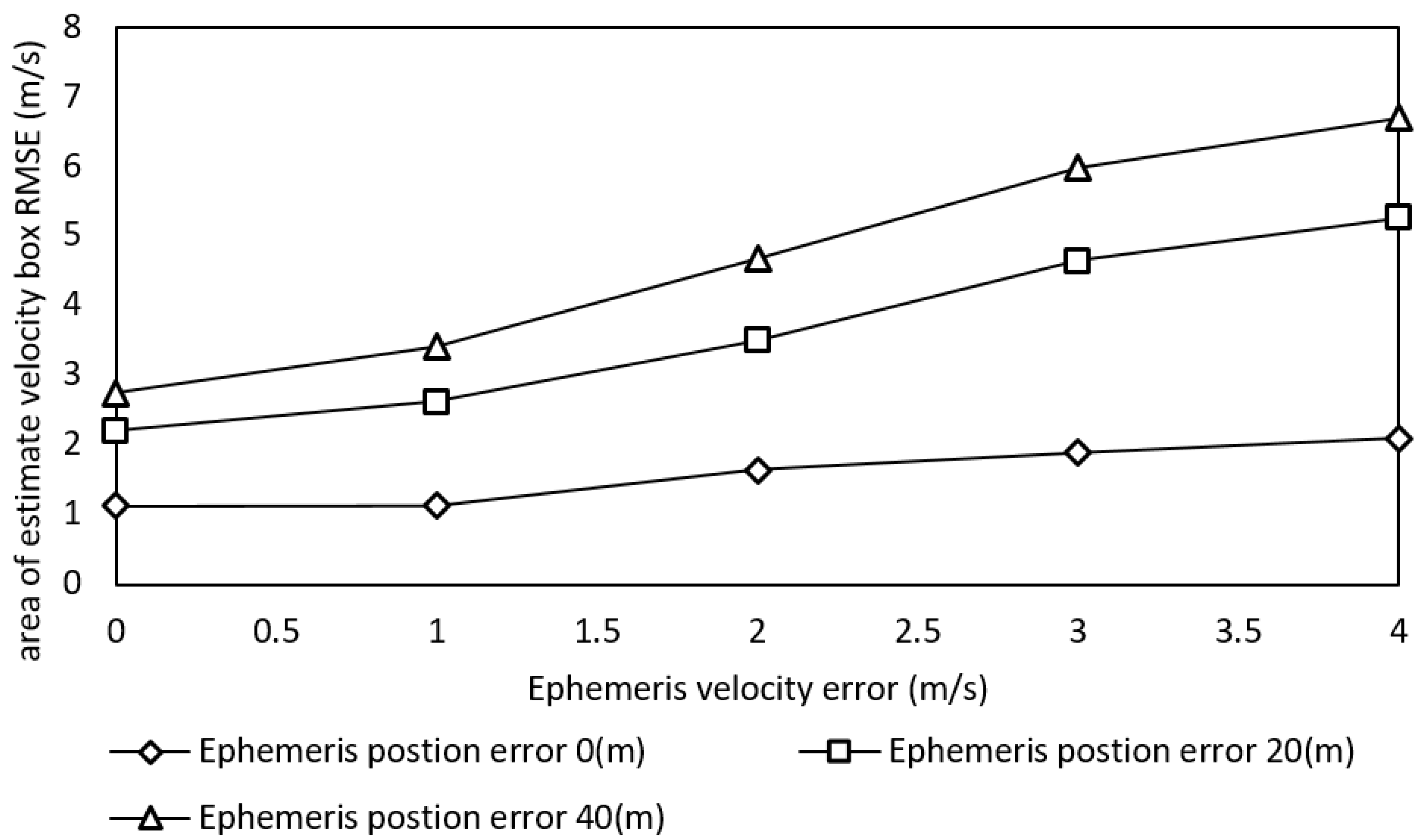
The effect of the ephemeris error on the velocity estimation interval is reflected in Figure 8 and Figure 9. It can be seen that in the case of the same ephemeris position error, the velocity estimation interval area increases with the increase of the ephemeris velocity error. When the ephemeris velocity error is the same, the velocity estimation interval area increases with the rise in the ephemeris position error. It can also be seen that although the RMSE of the velocity estimation interval increases with the increase of the ephemeris error, the deteriorating range is small which indicts the robustness of our proposed algorithm against the ephemeris position error.

In fact, when the ephemeris velocity error is beyond 2 m/s, the estimated velocity interval box area of the target will be as high as ten thousand (m/s)². Certainly, such error-level is not acceptable in the practical applications. However, the RMSE of the middle point is quite low, which is under 10 m/s in all cases. Nevertheless, the effect of the ephemeris position error on the interval area is not so obvious while it evidently has an apparent influence on the estimation accuracy, as shown in Figure 9.

4. Discussion

It is worthwhile to point out that the proposed interval calculation-based algorithm may prove to be a revolutionary methodology for the positioning and tracking research field. Our proposed method is free of the measurement distribution assumption, while most research works assume that the TDOA and FDOA measurements follow the Gaussian distribution which is not necessarily true. On the other hand, the estimated result is in a guaranteed interval form, which must include the ground truth. Additionally, the interval results are more convenient in performing the multiple system cooperation by the simple intersection calculation.

5. Conclusions

This paper introduces the interval analysis algorithm based on TDOA/FDOA joint location for the research of passive location. The variant formulas for calculating meridional velocity and zonal velocity are obtained through the frequency difference formula. When dividing the zonal velocity line and the meridional velocity line, the discrete point sets of meridional velocity and zonal velocity are obtained using the corresponding variant formula. Combined with the dichotomy algorithm, the velocity estimation interval is continuously reduced until the velocity estimation interval no longer shrinks, and a result interval including the actual velocity of the radiation source is obtained.

Several simulation experiments show that the inclusion rate can reach 100% in a certain error range, and the velocity estimation interval area is smaller, closer to the real value of the radiation source, and has higher accuracy and credibility. When the interval estimation comes to the midpoint, the calculated velocity estimation interval RMSE is relatively small, and the performance of the algorithm is rather good. Under the high error estimation, the RMSE does not fluctuate wildly, and the performance of the algorithm is still stable.

References

- Lee, K.; Oh, J.; You, K. TDOA-/FDOA-Based Adaptive Active Target Localization Using Iterated Dual-EKF Algorithm. IEEE Commun. Lett. 2019, 23, 752–755. [Google Scholar] [CrossRef]
- Zhou, B.; Ahn, D.; Lee, J.; Sun, C.; Ahmed, S.; Kim, Y. A Passive Tracking System Based on Geometric Constraints in Adaptive Wireless Sensor Networks. Sensors 2018, 18, 3276. [Google Scholar] [CrossRef] [PubMed] [Green Version]
- Wang, G.; Cai, S.; Li, Y.; Ansari, N. A Bias-Reduced Nonlinear WLS Method for TDOA/FDOA-Based Source Localization. IEEE Trans. Veh. Technol. 2015, 65, 8603–8615. [Google Scholar] [CrossRef]
- Liu, Z.; Wang, R.; Zhao, Y. A Bias Compensation Method for Distributed Moving Source Localization Using TDOA and FDOA with Sensor Location Errors. Sensors 2018, 18, 3747. [Google Scholar] [CrossRef] [PubMed] [Green Version]
- Congfeng, L.; Jinwei, Y.; Juan, S. Direct solution for fixed source location using well-posed TDOA and FDOA measurements. J. Syst. Eng. Electron. 2020, 31, 666–673. [Google Scholar] [CrossRef]
- Ho, K.C.; Xu, W. An accurate algebraic solution for moving source location using TDOA and FDOA measurements. IEEE Trans. Signal Process. 2004, 52, 2453–2463. [Google Scholar] [CrossRef]
- Wang, G.; Li, Y.; Ansari, N. A Semidefinite Relaxation Method for Source Localization Using TDOA and FDOA Measurements. IEEE Trans. Veh. Technol. 2013, 62, 853–862. [Google Scholar] [CrossRef]
- Wang, Y.; Wu, Y. An Efficient Semidefinite Relaxation Algorithm for Moving Source Localization Using TDOA and FDOA Measurements. IEEE Commun. Lett. 2017, 21, 80–83. [Google Scholar] [CrossRef]
- Qu, X.; Xie, L.; Tan, W. Iterative Constrained Weighted Least Squares Source Localization Using TDOA and FDOA Measurements. IEEE Trans. Signal Process. 2017, 65, 3990–4003. [Google Scholar] [CrossRef]
- Andrew, A.M. Applied Interval Analysis, with Examples in Parameter and State Estimation, Robust Control and Robotics; Springer: London, UK, 2001. [Google Scholar]
- Qin, N.; Wang, C.; Shan, C.; Yang, L. Interval analysis-based Bi-iterative algorithm for robust TDOA-FDOA moving source localisation. Int. J. Distrib. Sens. Netw. 2021, 17, 1–9. [Google Scholar] [CrossRef]
- Liu, S.; Han, C.; Di, R. Removal of attitude errors based on multi-target multi-sensor environment in earth-centered earth-fixed coordinates. In Proceedings of the 2010 International Conference on Information, Networking and Automation (ICINA), Kunming, China, 18–19 October 2010; pp. V2-10–V2-14. [Google Scholar]
Figure 1.
The coordinate system translation for the satellite-based positioning scenario.
Figure 2.
Interval contraction diagram.
Figure 3.
The result of the first iteration of the algorithm.
Figure 4.
The results of Step Two and Step Three of the algorithm.
Figure 5.
The final velocity estimation interval of the algorithm.
Figure 6.
The influence of TDOA and FDOA errors on the interval area of velocity estimation.
Figure 7.
The influence of TDOA and FDOA errors on the RMSE of velocity estimation.
Figure 8.
The influence of ephemeris error on the interval area of velocity estimation.
Figure 9.
The influence of ephemeris error on interval RMSE of velocity estimation.