A Neural Network-Based Interval Pattern Matcher

Abstract

One of the most important roles in the machine learning area is to classify, and neural networks are very important classifiers. However, traditional neural networks cannot identify intervals, let alone classify them. To improve their identification ability, we propose a neural network-based interval matcher in our paper. After summarizing the theoretical construction of the model, we take a simple and a practical weather forecasting experiment, which show that the recognizer accuracy reaches 100% and that is promising.

1. Introduction

Pattern recognition [1,2,3], which focuses on the recognition of patterns, is a branch of machine learning. In many cases, patterns are learned from training data, which is supervised learning, but when there is no training example provided, some pattern recognition algorithms can be used to discover previously unknown patterns, which is unsupervised learning [4,5,6].

Pattern recognition is to assign a class to a given input value or a set of values [7,8]. Generally speaking, pattern recognition algorithms aim to provide a reasonable answer for all possible inputs and to perform most likely matching of the inputs, taking into account their statistical variation. This is contrasted with pattern-matching algorithms, which look for exact output that matches to the input in a pre-existing pattern or patterns. A common example of a pattern-matching algorithm is regular expression matching [9,10,11]. In contrast to pattern recognition, pattern matching is generally not considered as a type of machine learning but a type of artificial intelligence, although pattern-matching algorithms can sometimes succeed in providing similar-quality output to the sort provided by pattern-recognition algorithms.

So far, there are some pattern-matching algorithms in the world, including ones for intervals. However, most of the interval-matching algorithms are used in much applied areas [12] and are highly related to specific features. In other words, these interval pattern matching methods are designed for specific problems, not for general ones.

The main contribution of the paper is to propose an interval pattern matcher that makes use of the neural network, and we call it a “neural network-based interval pattern matcher”. This pattern matcher has the property that can identify a mathematical interval, instead of a real number. Experiments illustrate that neural networks can form the core of the “Neural Network-based Interval Pattern matcher” that can identify the patterns more quickly compared with the pattern-matching algorithm using a searching method once the training process finishes.

The organization of this paper is as follows. In Section 2, we briefly introduce the preliminaries of the paper: neural networks. Section 3 describes the modeling of a neural network-based interval pattern matcher. Section 4 is the experiment to test the classifier that we propose. Finally, conclusions are given.

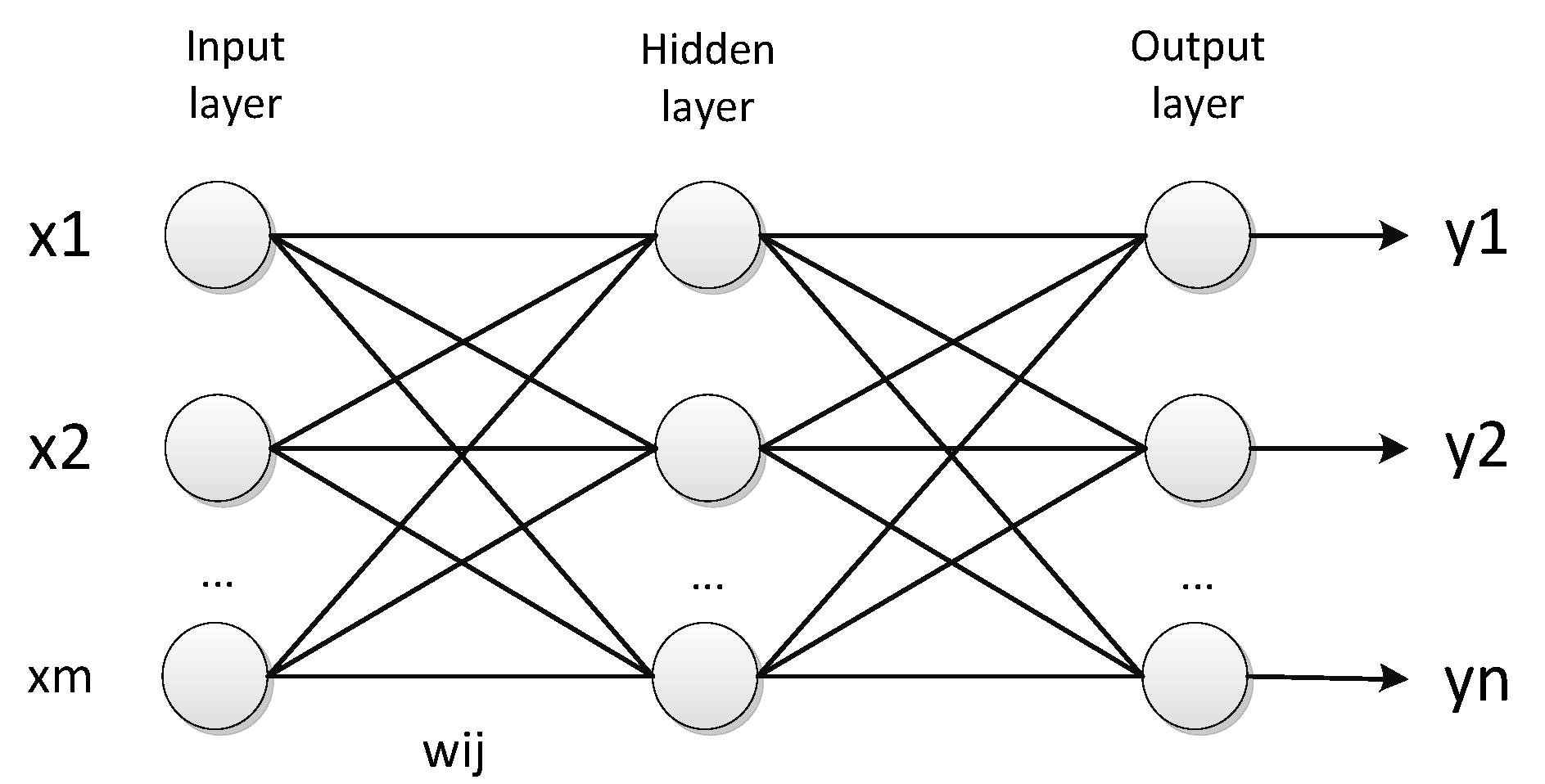
2. Preliminaries: Neural Networks

Artificial neural networks (shown in Figure 1) are electronic neuron structures that simulate the neural structure of the brain. They process one training sample at one time and learn by comparing real output with targets. The errors from the initial training step are used to modify the network weights the second time around, and so on. Roughly speaking, an artificial neural network is composed of a set of input values (x_i), associated weights (w_ij), and a function that sums the weights up and maps the results to the output vector (y). Neurons are organized into layers. The input layer is composed of neurons that represent the feature variable vector (x). The next layer is called the hidden layer; and there may be more than one hidden layer and more than one neuron in each hidden layer. The final layer is the output layer, where one node matches with one class for classification problems.

Figure 1. Artificial neural networks.

Figure 1. Artificial neural networks.

Neural network is an important tool for classification [13,14]. Basically, a classifier takes objects as inputs and assigns each one to a class; objects are represented as vectors of features and classes are represented as class labels, such as 0 or 1.

In the training phase, the correct class for each record is known, and the output nodes can therefore be assigned “class number” values—“1” for the node corresponding to the correct class, and “0” for the wrong class [15,16]. It is thus possible to compare the network's calculated output values with these “correct” (target) values, and calculate an error term for each node, which is the “Delta” rule. These errors are then used to adjust the weights in the hidden layers so that the output values will be closer to the “correct” (target) values for the next time. After the process of training, a single sweep forward through the network assigns a value to each output neuron, whose value is assigned to whichever class’s node had the highest value.

It is well-known that there are several types of neural networks, each of which has unique functions. In our paper, we focus on the pattern matching ability using a neural network, and come up with a pattern matcher that is a neural network with additional data preparation layer. The traditional neural network is typical enough to be used to in our system illustrate our problem.

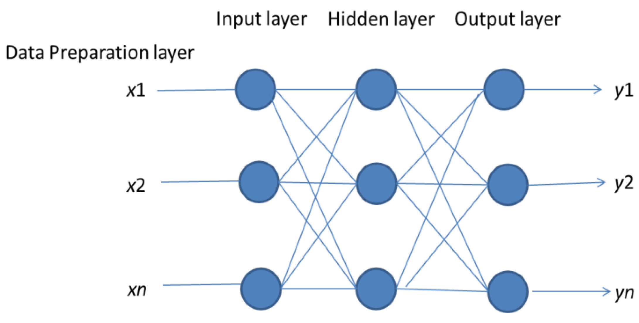
3. Neural Network-Based Interval Classifier

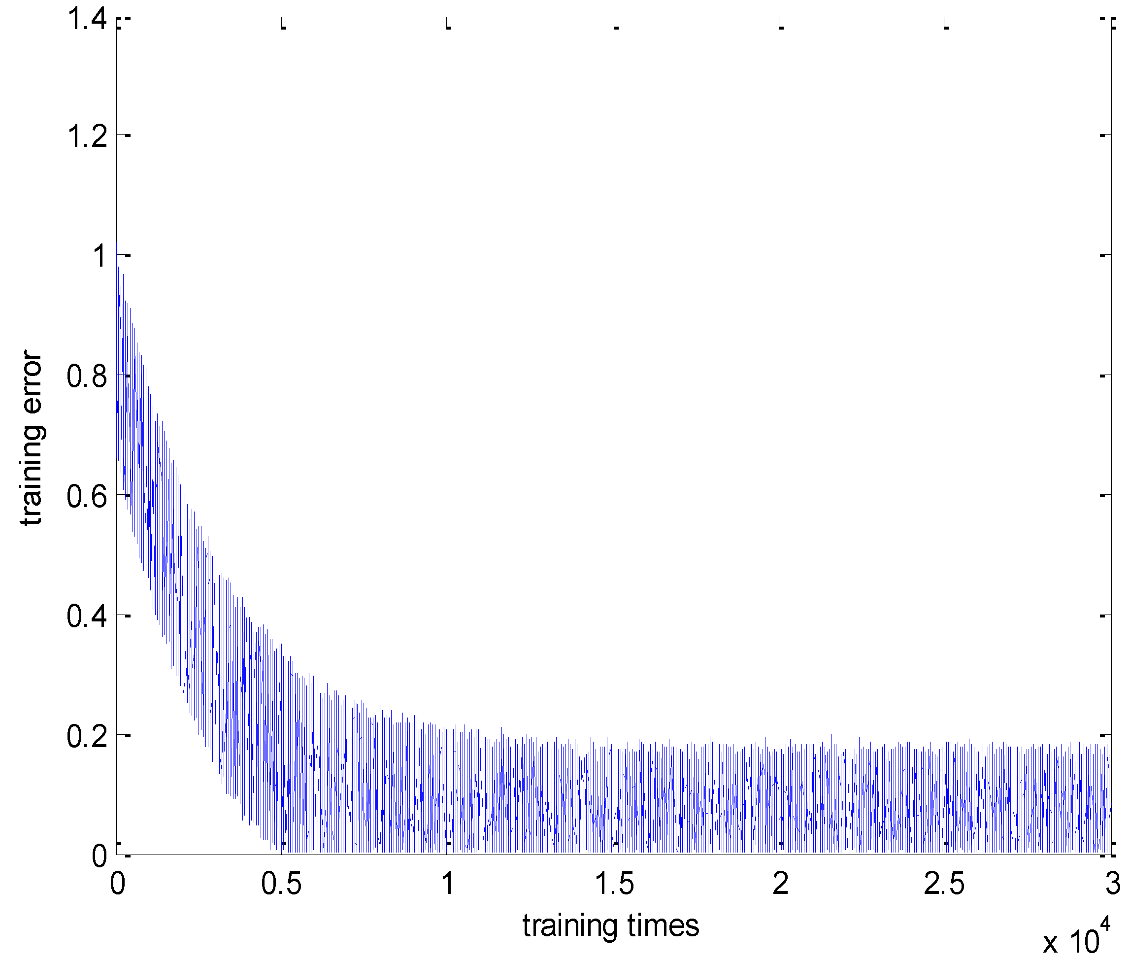
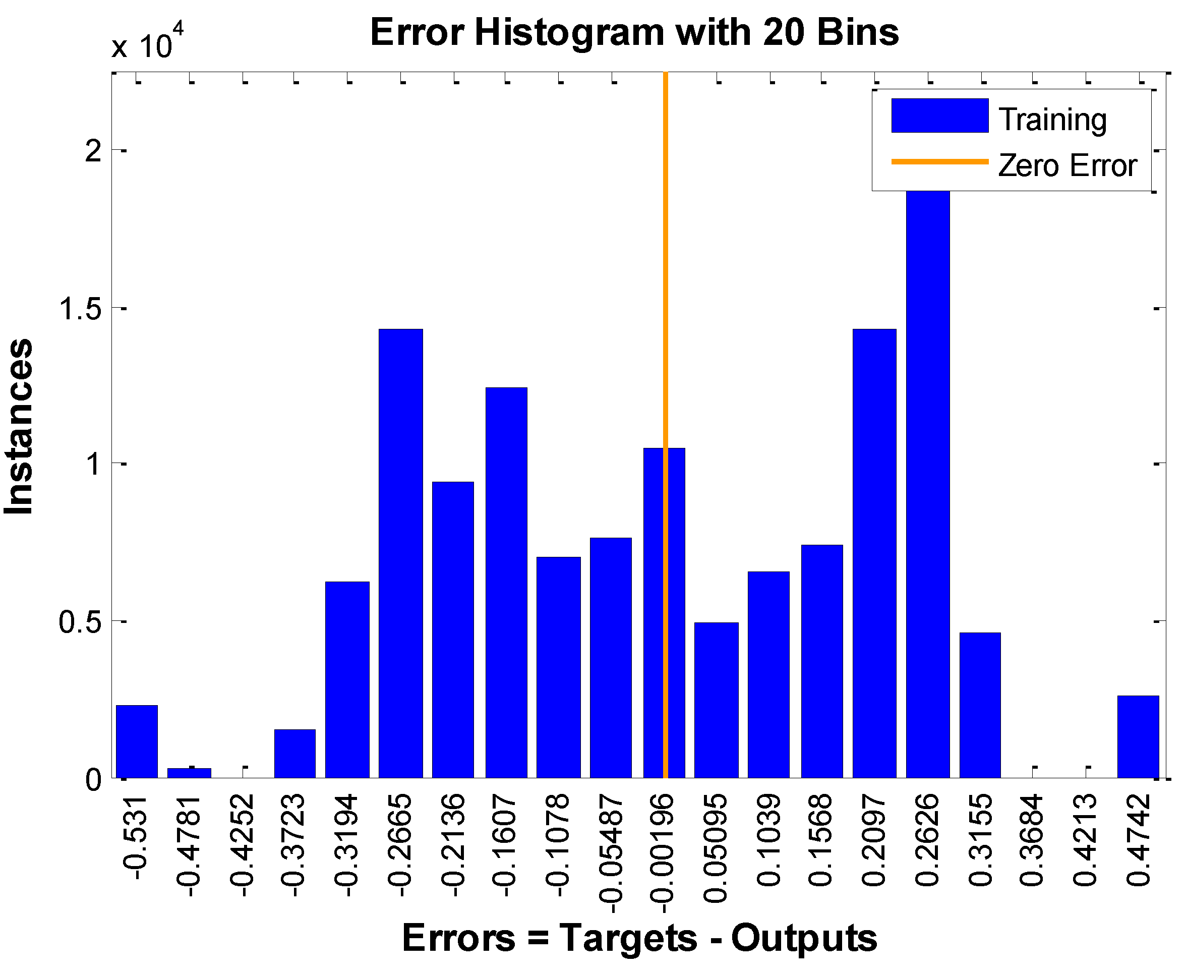
Rules [17,18,19] are often stated as linguistic IF-THEN constructions. It has the general form “IF A THEN B”, where A is called the premise of the rule and B is the consequence. We use (A; B) to denote this rule. Neural network can express such rule efficiently. However, it is more often seen that both A and B take a more complex form.

Take the simple rule set below as an example

(R₁) IF x₁ is Small AND x₂ is Small, THEN y is Small;

(R₂) IF x₁ is Small’ AND x₂ is Small’, THEN y is Small’.

There are two rules in this example, and the number of inputs is two. Small and Small’ denote intervals over the universe of x and y. R₁ can be denoted as (Small, Small; Small); R₂ can be denoted as (Small’, Small’; Small’).

Often, a continuous interval can be represented by some discrete examples. The discrete examples in the domain can be determined by interpolation. This idea reduces the processing complexity in our system using interval. For example, given the rule R₁, we need some specific value or (values) to depict the interval Small to minimize the complexity of it, neural network would face the difficulty that one input values would face more than one output value. Details are shown as the following:

If there is a one-to-many relationship between the inputs and targets in the training data, then it is not possible for any mapping to perform perfectly. One method is to calculate the average value for each interval. Any given network may or may not be able to approximate this mapping well at the beginning. However, it will form its best possible approximation to this mean output value when trained as well as possible.

One problem emerges when average features cannot distinguish one interval from the others. Sometimes, different intervals may have the same average values, especially for the intervals having overlap values. Whatever method we use, one interval should be distinguishable from the others on the limited domain related to the problem that we are trying to solve. For example, if our domain is {Large, Small, Middle}, we need to distinguish these three intervals but do not need to distinguish others.

Here, we have to emphasize the concept of “relation”. A “relation” is just a relationship among objects. If there are some persons in class and each person has their own height, the pair of one person and his/her name is a “relation”. Besides, these pairs are “ordered”, which means one comes first and the other comes second. The set of all the starting points is called “the domain” and the set of all the ending points is called “the range”.

What should we notice is that all functions are relations but not all relations are functions. A function is a sub-classification of relation and a well-behaved relation, we mean that, given a starting point, we know exactly where to go; given an x, we get only and exactly one y. The relation {(7,8;0), (7,8;1)} where “7” and “8” are input values and “0” and “1” are output values, is not a function since certain x-elements are paired with more than one unique y-element. However, the relation {(1;2), (3;2)} where “1” and “3” are input values and “2” is an output value, is a function since certain y-elements value can be paired with more than one unique x-element.

It is well known that a neural network can approximate a function very well [20,21,22], but it cannot express the one-many mapping correctly since the weight changes would be compromised between different outputs given the same inputs. In a traditional neural network, the training error of a function would approximate zero when trained as well as possible [23,24,25]; while for the non-function relation, the error does not converge to a real number, but rather to an interval.

For example, if we are given a relation {(1;2), (1;3)} and train the neural network using the training sample (1;2) and (1;3) alternately, at the beginning the weight change would simulate the relation (1;2) and then it would simulate the relation (1;3) and so forth. Thus, the weight changes would be a compromise among different outputs (“1” and “3”) given the same inputs (“1”) after a lot of iterations. When we input “1” to this well trained neural network, it would output a number between two and three randomly based on our research. Totally speaking, the range of the interval is closely related to the error interval.

Here, we make use of this error interval to decide if the training process is finished or not in the training process. Besides, we can also use this error interval and testing outputs to identify different interval output in the testing process. Specifically, the error interval would fall within an interval that is closely related to the error interval and output some values that fall within the interval itself. The network structure of this example is shown in Figure 2.

Figure 2. Neural network-based interval matcher.

Figure 2. Neural network-based interval matcher.

Specification:

Data preparation layer: This layer generates training samples from the raining rules. A suitable training sample is one which has values drawn from a distribution corresponding to a rule in the training rule base. (Training samples for rule R₁ must obey R₁.)

The main goal of the input layer is to generate some training samples randomly, each of which contains independent variable values (x₁, …, x_n) and values of the induced variable (y) that obey the corresponding rule. We generate values for each of the variables by drawing from a rule distribution [26,27,28].

Using the example from Section 3, there are two independent variable values (x₁, x₂) and one induced value y. To generate a training example for rule R₁, we would draw a sample for x₁ from the Small region of the domain of X₁; x₂ would be drawn from the Small region for X₂, and y would be drawn from the Small region of Y.

For example, we would like to approximate the relation (A,B;C), where A is {1,2}, B is {3,4} and C is {6,7}. We decompose this relation into (1,3;6), (1,3;7), (1,4;6), (1,4;7), (2,3;6), (2,3;7), (2,4;6), (2,4;7).

Input layer: This layer is similar to standard neural networks with inputs from the data preparation layer.

Hidden layer: The function of this layer is similar to standard neural networks, except that we have separate networks for each set of input classes. The training itself is done using the Back-Propagation algorithm. During training, a training sample is only used to train a single network in the neural training layer, not all of them.

Output layer: This layer outputs an interval values. if we input (1,3), (1,4), (2,3), (2,4), the output would be a number between 6 and 7 as would the others. Thus, we could estimate the interval C based on the outputs of the corresponding well trained neural network.

4. Experiments

4.1. Simple Test

4.1.1. Comparison Between Two Rules Using Our Program

The reason why we conduct this experiment is to testify that the range of the interval is closely related to the error interval. We tested the range solution on the simple rules R₁ and R₂:

Small is a set with the interval of [0, 10]. In other words, it is part of the “Small”. Table 1 depicts the experimental environment that we used for the tests.

Table 1. Experimental environment.

Algorithm to train the neural network	Back Propagation (BP) Algorithm
Neural network structure	4 layers having 3, 3, 3, and 1 neurons
Experiment tool	Matlab

Table 1. Experimental environment.

Algorithm to train the neural network	Back Propagation (BP) Algorithm
Neural network structure	4 layers having 3, 3, 3, and 1 neurons
Experiment tool	Matlab

We first test out the range solution on R₁. For this example, the universal of all three variables is the interval [0, 100]. To generate a test example, we simply generate a random three-tuple in [0, 100]3, and then check if this conforms to the stated rule R₁. (If it does not, we discard the training example.)

In this experiment, we generate 42,803 training samples that satisfied the R₁ in the rule set. Using 30,000 training samples to train the neural network, we get the error values shown below in Figure 3. Once the network finishes the training process, the error falls approximately within the interval [0–0.2].

Figure 3. Training error using range solution of R₁.

Figure 3. Training error using range solution of R₁.

Using the other 12,803 testing samples on the network, we get error values shown in Figure 4. We observe that the result approximately is between “0” to “0.2”. This means that the training process is successful and there is no over-fitting problem.

Figure 4. Training error using range solution of R₂.

Figure 4. Training error using range solution of R₂.

We used another rule R₂ to test the range solution. Using 20,000 training samples to train, the training error falls approximately within an interval [0, 0.08], as shown in Figure 5. Using the other 10,000 testing samples to test, the testing error falls approximately within an interval [0, 0.07], as shown in Figure 6.

Figure 5. Training error using “traingdx” of R₁.

Figure 5. Training error using “traingdx” of R₁.

Figure 6. Training error using “traingdx” of R₂.

Figure 6. Training error using “traingdx” of R₂.

It is observed that both rules’ training errors fall within an interval after getting a stable state, and the difference between the training errors of the two rules is the range of the error. The reason for this phenomenon is that the inputs of a training sample correspond to different output values. If the gap among the biggest output value and smallest output value is big, the range of the error is big; otherwise, the range of error is small.

Although the training error also falls within an interval for a function, the range of the interval will approach zero as long as the training times are sufficient. This is different from the non-function relation, whose training error range would not approach zero no matter how many training times the training process would take [28,29,30].

4.1.2. Comparison Between Two Rules Using Matlab Toolbox

Table 2 depicts the experimental environment that we used for the tests. We use “traingdx” to replace the general BP algorithm to test our results; use standard Matlab toolbox (version R2014a) to generate our results, instead of our own programming.

Table 2. Experimental environment.

Algorithm to train the neural network	Gradient descent with momentum and adaptive learning rate backpropagation algorithm (traingdx)
Neural network structure	4 layers having 3, 3, 3, and 1 neurons
Experiment tool	Matlab neural network tool box

Table 2. Experimental environment.

Algorithm to train the neural network	Gradient descent with momentum and adaptive learning rate backpropagation algorithm (traingdx)
Neural network structure	4 layers having 3, 3, 3, and 1 neurons
Experiment tool	Matlab neural network tool box

From Figure 5 and Figure 6, we see the results are in accord with the last experimental results. Specifically, if we rotate the Figure 5 and Figure 6 in clockwise direction about 90 degrees, these figures are almost the same as Figure 3 and Figure 4, respectively. With the increment of training times, the error would not decrease, but arrive to an interval, with the value vibrating within. The only difference is that Figure 5 and Figure 6 have negative errors but Figure 3 and Figure 4 do not. The reason for that is that we use absolute error to denote training errors.

4.2. Practical Test

From Shanxi Provincial Meteorological Bureau, China, we got the ground surface meteorological observation data in Taiyuan, a city of Shanxi Province, China from May 2007 to October 2007, May 2008 to October 2008 and May 2009 to October 2009, which are the rainy seasons in that city. The specific meteorological elements included the day’s atmospheric pressure, relative humidity, dry and wet bulb temperature, wind speed and accumulated precipitation at 8 p.m. (Beijing Time, equivalent to 1200 UTC), which we took into our experiments.

Table 3. Classification of input conditions.

Atmospheric pressure		Dry and wet bulb temperature		Relative humidity		Wind speed
Rating	Value (hPa)	Rating	Value (°C)	Rating	Value (%)	Rating	Value (MPH)
Moderate	>940	Lowest	<−10	Dry	[0, 30)	Calm	(0, 2)
Lower slightly	[930, 940)	Lower	[−10, 5)	Less dry	[30, 50)	Light Air	[2, 4)
		Moderate	[5, 30)	Less humid	[50, 70)	Light Breeze	[4, 7)
Lower	[920,930)	Higher	[30, 45)			Gentle Breeze	[7, 11)
Lowest	<920	Highest	>45	Humid	[70, 100]	Moderate Breeze	[11, 17)

Table 3. Classification of input conditions.

Atmospheric pressure		Dry and wet bulb temperature		Relative humidity		Wind speed
Rating	Value (hPa)	Rating	Value (°C)	Rating	Value (%)	Rating	Value (MPH)
Moderate	>940	Lowest	<−10	Dry	[0, 30)	Calm	(0, 2)
Lower slightly	[930, 940)	Lower	[−10, 5)	Less dry	[30, 50)	Light Air	[2, 4)
		Moderate	[5, 30)	Less humid	[50, 70)	Light Breeze	[4, 7)
Lower	[920,930)	Higher	[30, 45)			Gentle Breeze	[7, 11)
Lowest	<920	Highest	>45	Humid	[70, 100]	Moderate Breeze	[11, 17)

We took the day’s atmospheric pressure, relative humidity, dry and wet bulb temperature, and wind speed observations at 8 p.m. (Beijing Time) as input conditions. Before the experiments, we classified the input meteorological conditions into different intervals according to their rating, which is shown in Table 3. Atmospheric pressure falls into four intervals shown in the first two columns of Table 3; relative humidity falls into four intervals shown in the third and fourth columns; dry and wet bulb temperature falls into five intervals shown in the fifth and sixth columns; wind speed falls into five intervals shown in the last two columns.

We also took the accumulated precipitation in the next 24 hours as outputs for the weather prediction models and used the precipitation observations to verify our results. Precipitation falls into five levels shown in Table 4.

Table 4. Classification of precipitation outputs.

Precipitation rating	Precipitation value (mm)
Light rain	(0, 10.0)
Moderate rain	[10.0, 24.9)
Heavy rain	[24.9, 49.9)
Rainstorm	[49.9, 99.9)
Heavy rainstorm	[99.9, 249.0)

Table 4. Classification of precipitation outputs.

Precipitation rating	Precipitation value (mm)
Light rain	(0, 10.0)
Moderate rain	[10.0, 24.9)
Heavy rain	[24.9, 49.9)
Rainstorm	[49.9, 99.9)
Heavy rainstorm	[99.9, 249.0)

Experiments show that the accuracy of pattern matcher is 100%, which is promising.

5. Conclusions

This paper presents an interval pattern matcher that can identify patterns with interval elements using neural networks. Our new system is based on a traditional neural network, but unlike previous neural networks, our system can handle interval inputs values and interval output values. This model is more convenient for some applications when compared with systems that require single real inputs and outputs.

We show that the new system is suitable for interval pattern matching, which look for exact output that matches to the input in pre-existing pattern or patterns. That is, our system can identify intervals patterns and are better than other pattern matchers using searching algorithms when trained as well as possible, since search-based matcher have to spend extra time in searching. In addition, our system can identify interval-based patterns while previous neural networks can only deal with simple patterns with simple real number inputs and outputs.

Finally, experiments show that the error intervals are highly closed with the output: the bigger the interval output range, the bigger the error range. In addition, practical experiments shows that the accuracy of identification is 100%, which is promising.

As we know, the neural network can identify simple numbers, and we can now identify interval ones. This kind of matcher is important because most real world problems are better characterized by an interval rather than a single one.

References and Notes

1. Kawai, T.; Akira, S. The role of pattern-recognition receptors in innate immunity: Update on Toll-like receptors. Nat. Immunol. 2010, 11, 373–384. [Google Scholar] [CrossRef] [PubMed]
2. Takeuchi, O.; Akira, S. Pattern recognition receptors and inflammation. Cell 2010, 140, 805–820. [Google Scholar] [CrossRef] [PubMed]
3. Bunke, H.; Riesen, K. Recent advances in graph-based pattern recognition with applications in document analysis. Pattern Recognit. 2011, 44, 1057–1067. [Google Scholar] [CrossRef]
4. Wright, J.; Yi, M.; Mairal, J.; Sapiro, G.; Huang, T.S.; Yan, S. Sparse Representation for Computer Vision and Pattern Recognition. Proceed. IEEE 2010, 98, 1031–1044. [Google Scholar] [CrossRef]
5. Prest, A.; Schmid, C.; Ferrari, V. Weakly supervised learning of interactions between humans and objects. Pattern Anal. Mach. Intell. 2012, 34, 601–614. [Google Scholar] [CrossRef] [PubMed]
6. Gureckis, T.M.; Love, B.C. Towards a unified account of supervised and unsupervised category learning. J. Exp. Theor. Artif. Intell. 2003, 15, 1–24. [Google Scholar] [CrossRef]
7. Ulbricht, C.; Dorffner, G.; Lee, A. Neural networks for recognizing patterns in cardiotocograms. Artif. Intell. Med. 1998, 12, 271–284. [Google Scholar] [CrossRef]
8. Saba, T.; Rehman, A. Effects of artificially intelligent tools on pattern recognition. Int. J. Mach. Learn. Cybern. 2013, 4, 155–162. [Google Scholar] [CrossRef]
9. Pedro, J.; García-Laencina, J.S.; Figueiras-Vidal, A.R. Pattern classification with missing data: A review. Neural Comput. Appl. 2010, 19, 263–282. [Google Scholar]
10. Santos, A.; Powell, J.A.; Hinks, J. Using pattern matching for the international benchmarking of production practices. Benchmarking: Int. J. 2001, 8, 35–47. [Google Scholar] [CrossRef]
11. Ficara, D.; Di Pietro, A.; Giordano, S.; Procissi, G.; Vitucci, F.; Antichi, G. Differential encoding of DFAs for fast regular expression matching. IEEE/ACM Trans. Netw. 2011, 19, 683–694. [Google Scholar] [CrossRef]
12. Huang, J.; Berger, T. Delay analysis of interval-searching contention resolution algorithms. IEEE Trans. Inf. Theoy. 1985, 31, 264–273. [Google Scholar] [CrossRef]
13. Lin, C.; Chang, S. Efficient pattern matching algorithm for memory architecture. IEEE Trans. Very Larg. Scale Integr. Syst. 2011, 19, 33–41. [Google Scholar] [CrossRef]
14. Yuan, H.; Wiele, C.F.V.D.; Khorram, S. An Automated Artificial Neural Network System for Land Use/Land Cover Classification from Landsat TM Imagery. Remote Sens. 2009, 1, 243–265. [Google Scholar] [CrossRef]
15. Levine, E.R.; Kimes, D.S.; Sigillito, V.G. Classifying soil structure using neural networks. Ecol. Model. 1996, 92, 101–108. [Google Scholar] [CrossRef]
16. Liu, H.; Chen, Y.; Peng, X.; Xie, J. A classification method of glass defect based on multiresolution and information fusion. Int. J. Adv. Manuf. Technol. 2011, 56, 1079–1090. [Google Scholar] [CrossRef]
17. Chao, W.; Lai, H.; Shih, Y.I.; Chen, Y.; Lo, Y.; Line, S.; Tsang, S.; Wu, R.; Jaw, F. Correction of inhomogeneous magnetic resonance images using multiscale retinex for segmentation accuracy improvement. Biomed. Signal Process. Control 2012, 7, 129–140. [Google Scholar] [CrossRef]
18. Özbay, Y.; Ceylan, R.; Karlik, B. Integration of type-2 fuzzy clustering and wavelet transform in a neural network based ECG classifier. Expert Syst. Appl. 2011, 38, 1004–1010. [Google Scholar] [CrossRef]
19. Orhan, U.; Hekim, M.; Ozer, M. EEG signals classification using the K-means clustering and a multilayer perceptron neural network model. Expert Syst. Appl. 2011, 38, 13475–13481. [Google Scholar] [CrossRef]
20. Chen, L.; Liu, C.; Chiu, H. A neural network based approach for sentiment classification in the blogosphere. J. Informetr. 2011, 5, 313–322. [Google Scholar] [CrossRef]
21. Mohamed, A.; Dahl, G.E.; Hinton, G. Acoustic modeling using deep belief networks. IEEE Trans. Audio Speech Lang. Process. 2012, 20, 14–22. [Google Scholar] [CrossRef]
22. Feuring, T.; Lippe, W. The fuzzy neural network approximation lemma. Fuzzy Sets Syst. 1999, 102, 227–236. [Google Scholar] [CrossRef]
23. Karlik, B.; Olgac, A.V. Performance analysis of various activation functions in generalized MLP architectures of neural networks. Int. J. Artif. Intell. Expert Syst. 2011, 1, 111–122. [Google Scholar]
24. Krizhevsky, A.; Sutskever, I.; Hinton, G.E. Imagenet classification with deep convolutional neural networks. Adv. Neural Inf. Process. Syst. 2012, 1, 1097–1105. [Google Scholar]
25. Hasiewicz, Z. Modular neural networks for non-linearity recovering by the Haar approximation. Neural Netw. 2000, 13, 1107–1133. [Google Scholar] [CrossRef]
26. Lee, H.K.H. Consistency of posterior distributions for neural networks. Neural Netw. 2000, 13, 1107–1133. [Google Scholar] [CrossRef]
27. Erhan, D.; Bengio, Y.; Courville, A. Why does unsupervised pre-training help deep learning? J. Mach. Learn. Res. 2010, 11, 625–660. [Google Scholar]
28. Shao, Y.; Lunetta, R.S. Comparison of support vector machine, neural network, and CART algorithms for the land-cover classification using limited training data points. ISPRS J. Photogramm. Remote Sens. 2012, 70, 78–87. [Google Scholar] [CrossRef]
29. McCormack, L.; Dutkowski, P.; El-Badry, A.M. Liver transplantation using fatty livers: Always feasible? J. Hepatol. 2011, 54, 1055–1062. [Google Scholar] [CrossRef] [PubMed]
30. Cortes, M.; Pareja, E.; García-Cañaveras, J.C. Metabolomics discloses donor liver biomarkers associated with early allograft dysfunction. J. Hepatol. 2014, 61, 564–574. [Google Scholar] [CrossRef] [PubMed]
31. Lloyd, C.; Grossman, A. The AIP (aryl hydrocarbon receptor-interacting protein) gene and its relation to the pathogenesis of pituitary adenomas. Endocrine 2014, 46, 387–396. [Google Scholar] [CrossRef] [PubMed]