Article

Classifying the Degree of Bark Beetle-Induced Damage on Fir (Abies mariesii) Forests, from UAV-Acquired RGB Images

by
Tobias Leidemer
1,*,
Orou Berme Herve Gonroudobou
2,
Ha Trang Nguyen
2,
Chiara Ferracini
3,
Benjamin Burkhard
1,
Yago Diez
4 and
Maximo Larry Lopez Caceres
2
1
Institute of Physical Geography Landscape Ecology, Leibniz University of Hannover, Schneiderberg 50, 30167 Hannover, Germany
2
Faculty of Agriculture, Yamagata University, Tsuruoka 997-8555, Japan
3
Department of Agricultural, Forest and Food Sciences (DISAFA), University of Torino, Largo Paolo Braccini 2, 10095 Grugliasco, Italy
4
Faculty of Science, Yamagata University, Yamagata 990-8560, Japan
*
Author to whom correspondence should be addressed.
Submission received: 9 February 2022 / Revised: 11 April 2022 / Accepted: 14 April 2022 / Published: 18 April 2022
(This article belongs to the Special Issue Computation and Analysis of Remote Sensing Imagery and Image Motion)

Abstract

:
Bark beetle outbreaks are responsible for the loss of large areas of forests and in recent years they appear to be increasing in frequency and magnitude as a result of climate change. The aim of this study is to develop a new standardized methodology for the automatic detection of the degree of damage on single fir trees caused by bark beetle attacks using a simple GIS-based model. The classification approach is based on the degree of tree canopy defoliation observed (white pixels) in the UAV-acquired very high resolution RGB orthophotos. We defined six degrees (categories) of damage (healthy, four infested levels and dead) based on the ratio of white pixel to the total number of pixels of a given tree canopy. Category 1: <2.5% (no defoliation); Category 2: 2.5–10% (very low defoliation); Category 3: 10–25% (low defoliation); Category 4: 25–50% (medium defoliation); Category 5: 50–75% (high defoliation), and finally Category 6: >75% (dead). The definition of “white pixel” is crucial, since light conditions during image acquisition drastically affect pixel values. Thus, whiteness was defined as the ratio of red pixel value to the blue pixel value of every single pixel in relation to the ratio of the mean red and mean blue value of the whole orthomosaic. The results show that in an area of 4 ha, out of the 1376 trees, 277 were healthy, 948 were infested (Cat 2, 628; Cat 3, 244; Cat 4, 64; Cat 5, 12), and 151 were dead (Cat 6). The validation led to an average precision of 62%, with Cat 1 and Cat 6 reaching a precision of 73% and 94%, respectively.

1. Introduction

Bark beetle outbreaks are responsible for the loss of large areas of forests all over the world with irreversible changes on the landscape and significant economical loses. Bark beetle outbreaks reduce wood quality and production and influence the water/nutrient/carbon cycle, affecting ecosystem biodiversity [1,2]. In recent years, such pest outbreaks in forests appear to be increasing in frequency and magnitude all over the world as a result of climate change [2]. The probability of bark beetle attacks increases after long periods of drought, storms, windthrows [3,4], heavy snow, and other extreme weather conditions that weaken trees, making them ideal breeding grounds [5,6,7]. Once they have reached high population levels, bark beetles are even able to attack and infest healthy trees, as is the case of mountain pine beetles, which can cause the mortality of apparently healthy trees over millions of hectares [8]. In Japan, as in the rest of Asia, including Eurasia in Russia, the main common bark beetle is Polygraphus proximus [9], which is a non-aggressive phloephagous reaching a size of up to 12 mm. In 2013, a large-scale outbreak of P. proximus took place in Zao Mountains in northeastern Japan that, by 2016, had already devastated hundreds of hectares of pristine fir forests [10]. Since the area affected is part of a Quasi-National Park, the application of chemicals or any harmful material is forbidden and thus, the spread of bark beetles has been left undisturbed. This in turn, offers an excellent ground to monitor the natural process of bark beetle spread, forest resilience, and the role of abiotic factors in ameliorating or enhancing its effect. There are two common approaches that are used to evaluate the effect of bark beetles on forests, fieldwork observations and satellite images (usually hyperspectral ones). The first one is limited in space and the second one, even though it covers large areas at once, is limited in its precision since the medium resolution used ranges from 10 m to 100 m as is the case for Landsat images, although high resolution data (1–10 m) have been commonly used for further supporting detail mapping of the temporal effect of bark beetles [11], with very few of these studies conducted in Asia [12]. In order to monitor the development of damage at the individual tree level and the mapping of the whole affected forest area, it is necessary to quantify the number of infested trees and classify the degree of damage of each one of them. The most frequently used indexes for mapping bark beetle disturbances are the Enhanced Wetness Difference Index (EWDI), followed by the Normalized Burn Ratio (NBR) and Disturbance Index (DI) [11]. From these indexes, classifications, such as severely infested or almost dead, provide a qualitative but not a quantitative description of the damage and they cannot be used easily for comparison with other forest stands. It is also inaccurate to point to areas of infestation in coarse resolution images (>100 m) when the areas enclosed in large pixels could still include healthy trees [2,13]. Furthermore, the classification of the degree of damage of individual trees during field observations is subject to human criteria, experience, and accessibility to the tree canopy being classified, especially in highly dense forests [14,15]. Thus, the results are usually difficult to validate and compare with other forest stands, unless the same person and the same conditions are met, which is physically impossible, especially when the limited area the assessor can cover is considered. From fieldwork surveys as well as remote sensing studies, there is no standard criteria that can be used for comparison, first, because the patterns of damage are not discussed, and second, because there is no quantification of the degree of damage of single trees in time or space. In recent years, there have been several studies using unmanned aerial vehicles (UAV)-acquired images to evaluate and monitor forest pest infestation, mainly using hyperspectral cameras [16,17] and rarely RGB cameras [10,18]. In these latter two studies, the obtained data were also used to train deep learning models for tree health status detection. In both studies, the question was whether trees were healthy, infested, or dead. UAVs have shown an immense potential to close the gap between field observations and satellite imagery [19], since its low elevation flights produce very high-resolution images (0.02–0.03 m) and can cover areas of several tens to hundreds of hectares. The very high-resolution data have renewed interest in the use of a wide variety of data processing techniques, which include computer vision, soft computing, and deep learning [10,14,20,21,22] among others. Furthermore, pixel counting in satellite images to estimate classes in a given area [23] can be used at a micro level for counting pixels to estimate defoliation in a given tree canopy area from very-high resolution images. Thus, the aims of this study are: (1) to identify the health condition of fir trees from UAV-acquired RGB images; and (2) quantify and classify the degree of damage caused by bark beetle infestation in single fir trees inferred from the white pixels of partially or completely defoliated tree branches.

2. Material and Methods
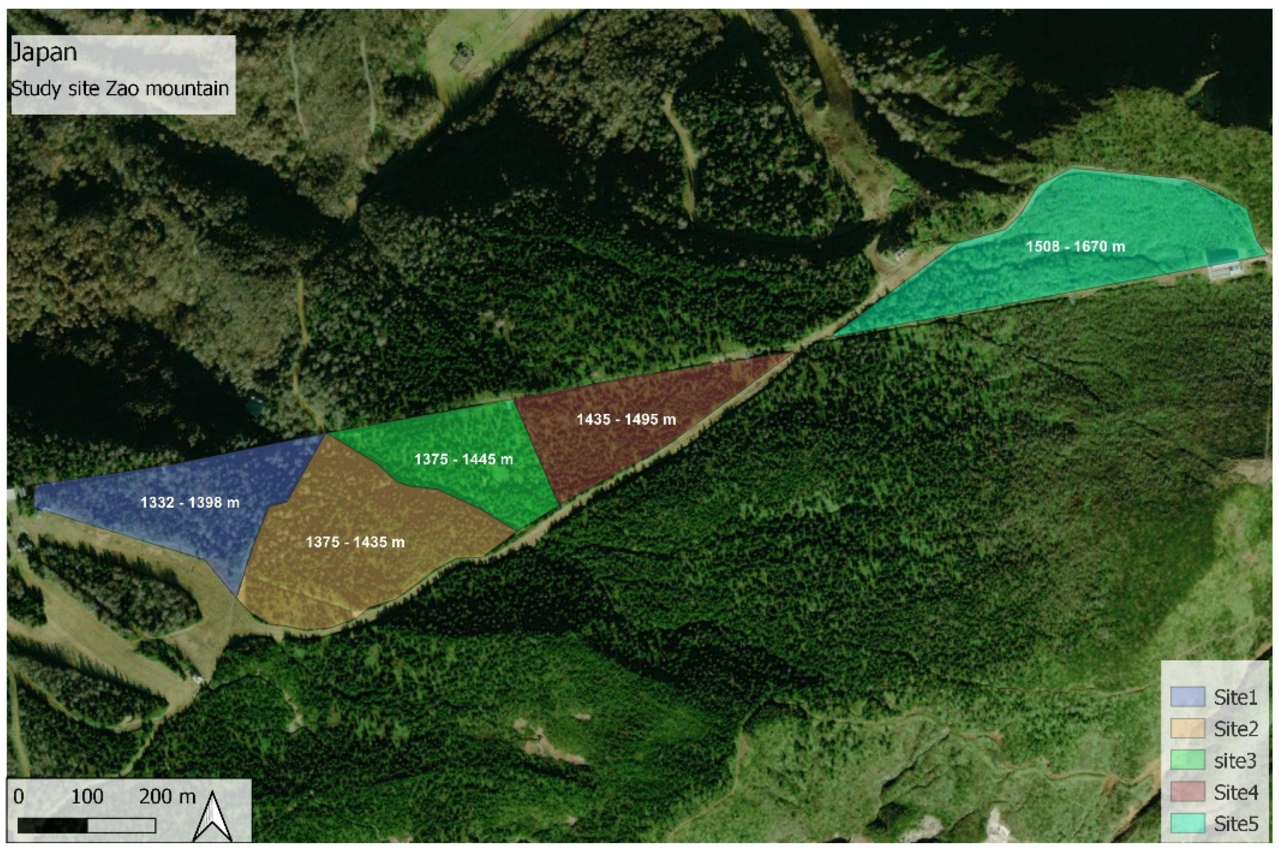
2.1. Study Site

The study area is located in Zao Mountains, a volcano in southeastern Yamagata, Japan (38°09′05” N, 140°25′03” E). The site covers an area of 25 ha with a tree density of about 200 trees/ha. The age of fir trees in the area ranges from 41 to 103 years old. The study area is divided into five sites in which the degree of insect damage along an elevation gradient of 1332 m to 1670 m (Figure 1) is evaluated. Site 1 (3.9 ha) is in the lower elevation and site 5 (6 ha) is in the highest elevation. Site 1 and site 2 are composed of Maries fir mixed with other deciduous tree species such as: Acer spp., Fagus crenata and Sorbaria sorbifolia. However, with increasing altitude, the number of deciduous tree species decreases and fir becomes the dominant tree species. Thus, in sites 3 (5.1 ha) and 4 (4 ha), fir is the dominant tree species. In site 5 (1508–1670 m), 95% of all fir trees are dead [11].

2.2. Data Acquisition

Sets of RGB aerial photos were collected during the growing season of the years 2020 and 2021. Several flight-missions were conducted with a DJI Mavic 2 pro Hasselblad L1D-20c camera. The UAV acquired 20-megapixel images, following routes designed on DJI GS pro software (DJI Inc., Shenzhen, China). The camera sensor is a 1-inch CMOS with fixed focal length of 10 mm and aperture f/3.2. The UAV flew at 70 m altitude from take-off points, nadir view, 3 m/s and shutter interval of 2 s. The photos were acquired with 90% side and front overlap. The camera was set at S priority (ISO-100) with shutter speed at 1/240–1/320 s in the case of strong sun and wind and at 1/80–1/120 in more favorable weather conditions. This setup kept exposure values (EV) of around 0 to +0.7 providing a ground sampling distance (GSD) of 1.5–2.1 cm/pixel. Other missions used a DJI Phantom 4 Quadcopter. The camera sensor in this UAV is 1/2.3-inch CMOS with fixed focal length of 24 mm. The UAV flew at speed 2 m/s, with a shutter interval of 2 s. The camera was set in automatic mode at a shutter speed of 1/120 s, ISO-100, EV at 0. This set up resulted in a GSD of 2.6 cm/pixel. The number of RAW images of each flight mission ranged from 150 to 390 [11].

2.3. Data and Programs

The orthomosaics had a pixel size of 0.014 m to 0.02 m and were delivered in JPG-format or tiff. They had 3–4 bands, but were generalized by a program to a 3-band data. Moreover, the sizes were standardized to a size of 0.02 m time 0.02 m. The coordinate system was Tokyo_UTM_Zone_54N. The programs that were used in this study were ArcGIS Pro version 2.7.0, python 3.7, and spyder 3.3.6. All programs were run under a Microsoft Windows 10 64-bit operating system. Nineteen different orthomosaics were collected under different environmental conditions for this study (Table 1).

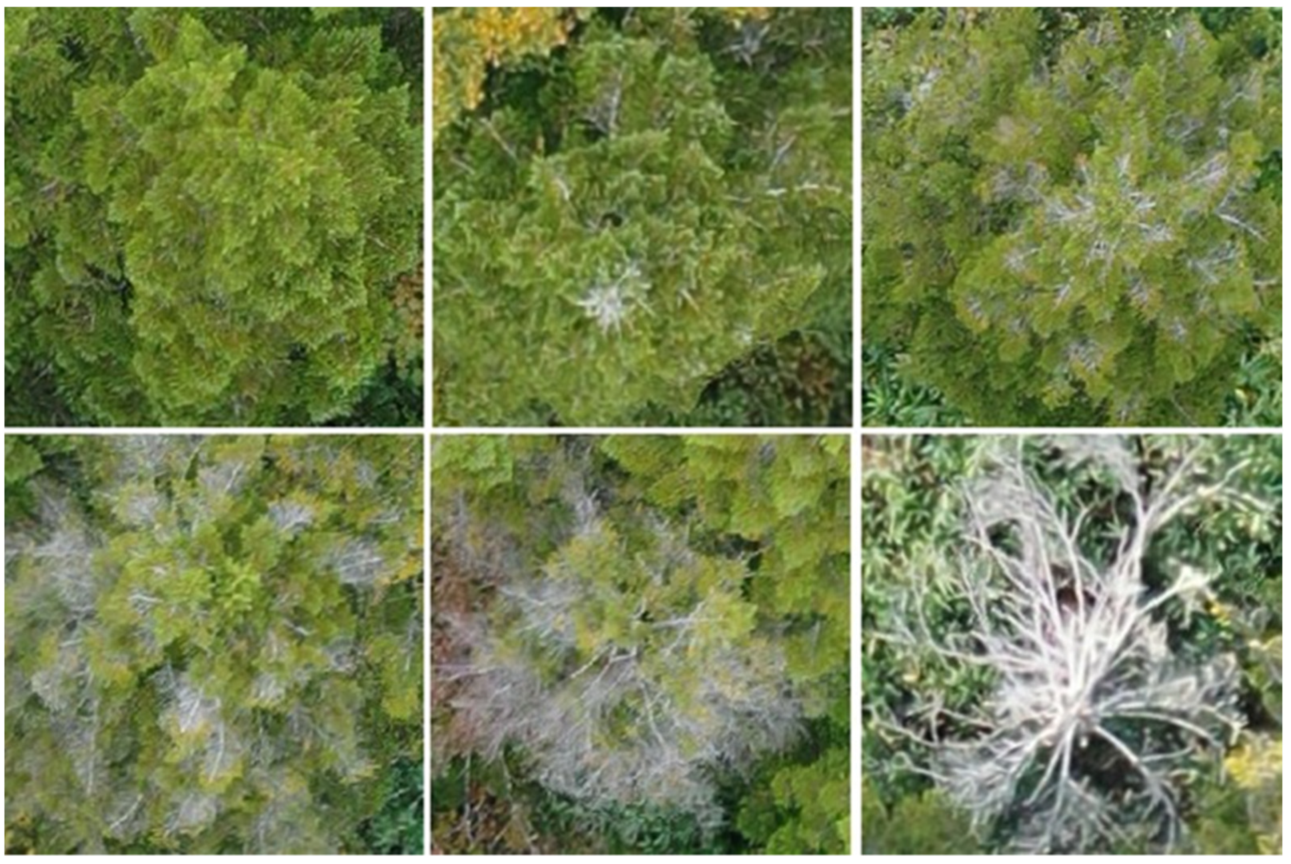
2.4. Definition of Tree Health Category

Based on these images, the degree of defoliation in individual trees is evaluated. The most relevant visual symptom of tree infestation from UAV-acquired images is the whitish looking leafless branches in random areas within the canopy. The percentage of white pixels increases with the degree of tree defoliation (health decline), from full green when the tree is healthy (non-infested) to full white when the tree is dead or completely defoliated (Figure 2).
Thus, the canopy area of each tree is divided into pixels of 0.02 × 0.02 m size each, of which the white pixels represent the defoliated branches in each tree. The proportion of white pixels to the total number of pixels (white and non-white) within the tree canopy is calculated and classified into six different categories, representing the degree of defoliation of any given tree: Cat 1: <2.5% (healthy, no defoliation); Cat 2: 2.5–10% (very low defoliation); Cat 3: 10–25% (low defoliation); Cat 4: 25–50% (medium defoliation); Cat 5: 50–75% (high defoliation), and finally Cat 6: >75% (dead), based on the classification of [15].

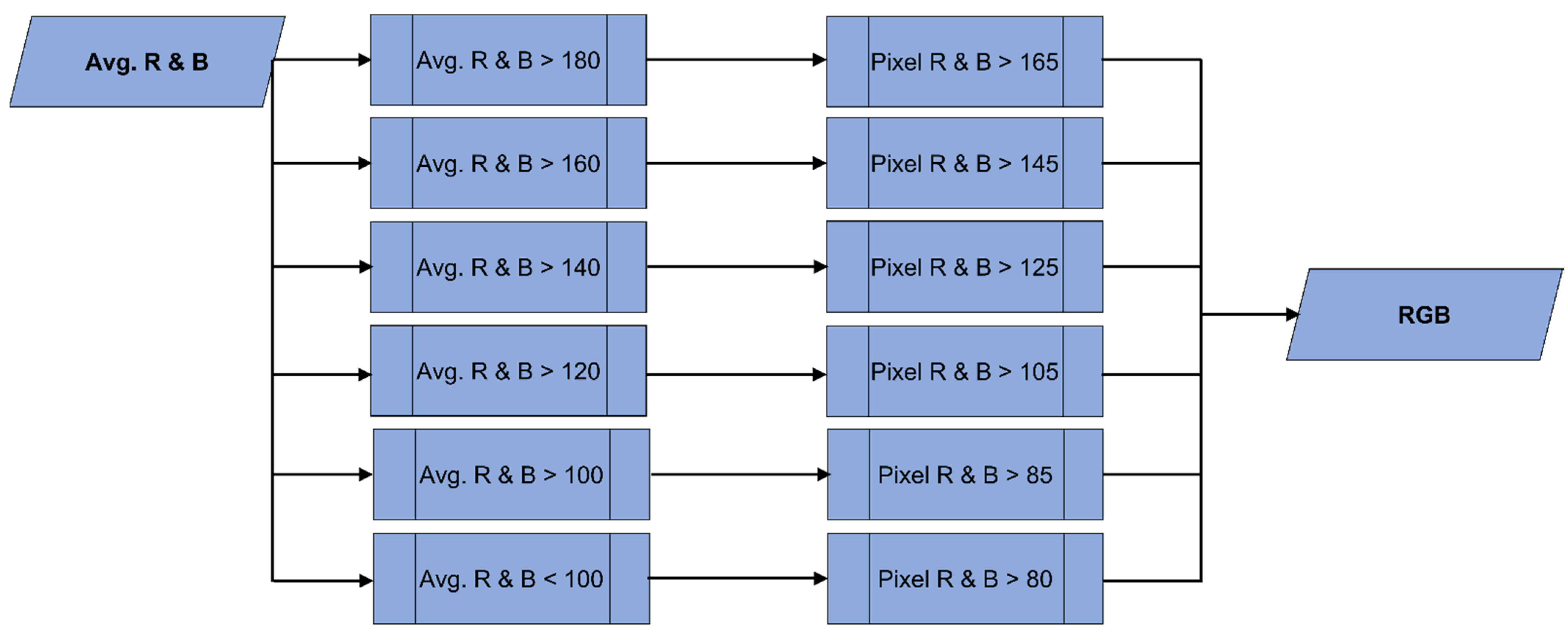
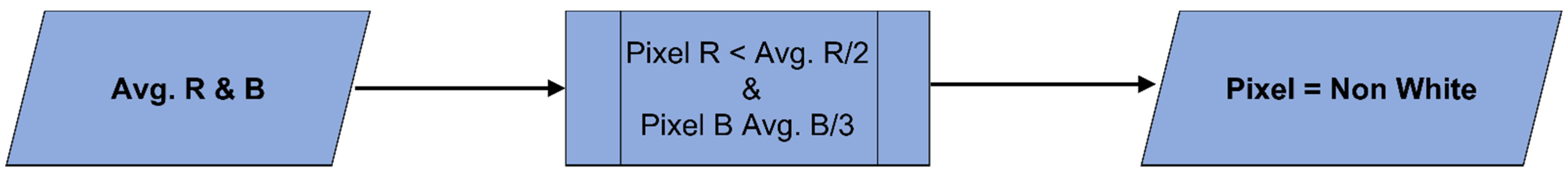
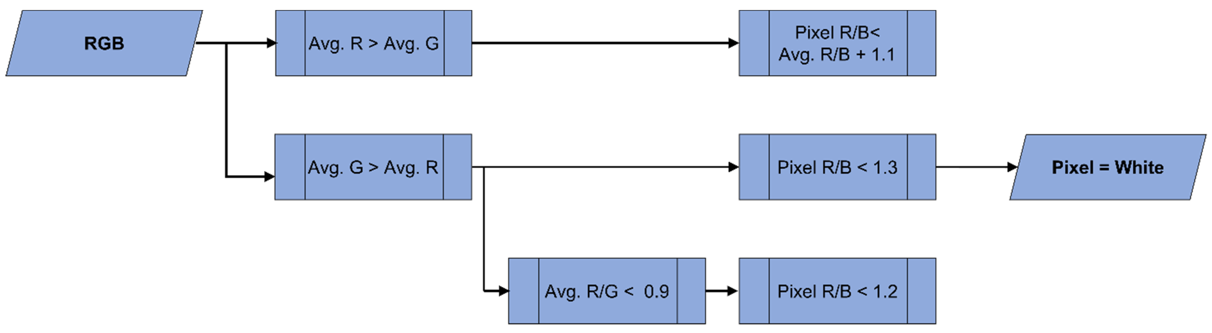
2.5. Calculation of Whiteness

The whiteness of each pixel is defined by the RGB-color system and its values. The color white consists of an equal proportion of the colors red, green and blue, with relatively high color values. As these values decrease, keeping the same ratio among them, the white changes to gray and then to black. However, depending on the light conditions during the collection of the images that were used for the different orthomosaics, the values and ratios for the white color varies considerably. Thus, in order to determine white and non-white pixels within the tree canopy, we carried out the following three steps:
First, a pixel is considered white if the red (R) and blue (B) pixel values are higher than the average R and B pixel values of the whole orthomosaic. By considering the average value of the orthomosaic when defining white and non-white, different orthomosaics that were made with images collected under different light conditions can be compared. The ratio of the R and B values is used, because from successive tests, it was found that blue is the decisive value when the pixel is white. When the color value approaches white, the blue value increases and reaches similar values as the red values.
Since each orthomosaic has different light characteristics, the average R and B values are different for each of the 19 orthomosaics. In the orthomosaics used in this study, the average R and B values ranged from 100 to 180 (Figure 3). Thus, for each orthomosaic, the threshold values were different. Since, after several trial-and-error tests, the threshold values of the averaged R and B values left some white pixels out, we decided to homogeneously decrease the threshold values 15 points in each orthomosaic. As a result, the model could identify clearly the white pixels in each orthomosaic regardless of the lightning conditions at which the images for a given orthomosaic were collected.
Second, we focus on the pixels that were considered non-white in the first step. If the pixel values of R and B, are lower than the average B pixel values divided by 3 and R pixel values divided by 2, then the pixel is considered as non-white (Figure 4). The reason for dividing R by 2 and B by 3 is that the red value is usually much higher (pixel values) than that of blue. Therefore, the dividend must be set lower, resulting in a higher absolute minimum threshold value. It is important that as many non-white pixels are included as possible leaving white pixels out. Non-white pixels include green areas (foliated branches) of the tree, as well as dark pixels that are not part of the canopy, which might otherwise be defined as one in the next step.
For the final step, the ratio between the R and the B pixel value (R/B) is calculated. First, we determine the average red and green (G) color values and the ratio between them. If the ratio is higher than 1, red is the dominant color, but if green is the dominant color, the ratio is lower than 1. Thus, threshold ratios must be adjusted. When the average R is higher than the average G, and the R/B ratio value of an individual pixel is lower than 1.3, then the pixel is considered as white. However, if the ratio between R and G pixel values (R/G) is smaller than 0.9, then the pixel R/B ratio should be lower than 1.2 to be considered as white. If the average R pixel value is higher than the average G pixel value, then pixels with an R/B ratio lower than 1.1 are considered as white (Figure 5). Under all other conditions, the pixel is considered as non-white. The R/B ratio was chosen because there are large variations between these two colors. Once all pixels have been categorized as white or non-white, then the model calculates how many white pixels are part of the area of the tree. Every white pixel is assigned the value 1, while all the non-white pixels are assigned the value 0. These steps are repeated for each individual pixel of a given orthomosaic. The result is a grid shape with 1 s and 0 s and then by using steps one, two, and three, the threshold errors are also minimized.

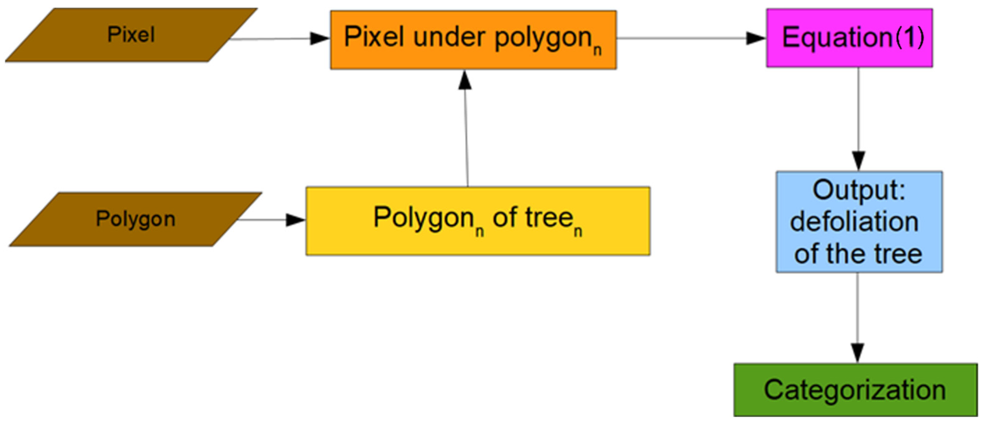
2.6. Polygon Definition
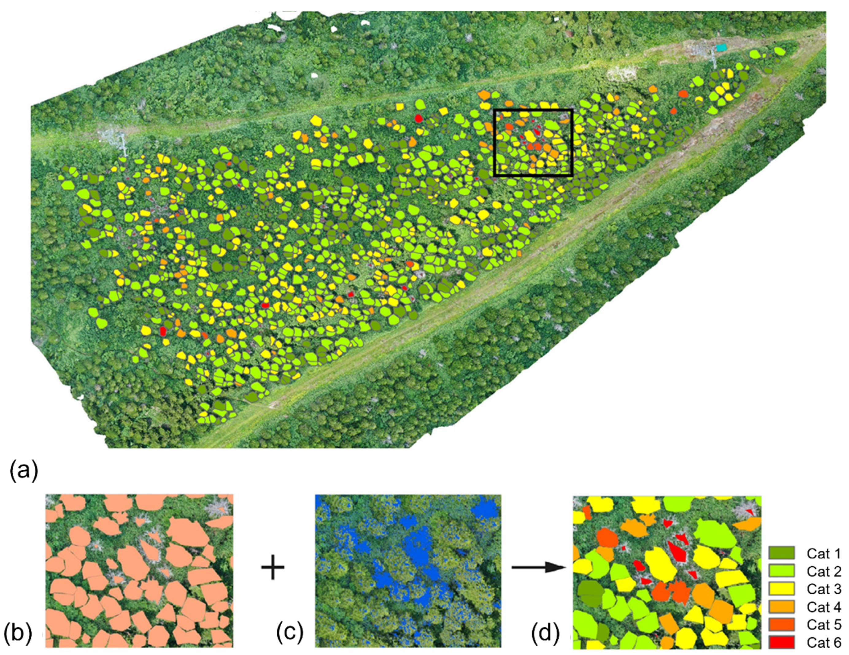
Polygons were drawn around every single fir tree and saved in a shape file. In this study, the polygons were drawn manually. There was a careful consideration for polygons to include as much area from the tree and as little of the non-tree area as possible to make sure that each tree canopy area was correctly represented. The number of white (1) and non-white pixels (0) are counted for each polygon using Equation (1).
Proportion   of   whiteness = P i x e l w h i t e P i x e l
where ∑Pixelwhite is the sum of all white pixels of the canopy area from a single tree and ∑Pixel is the number of all pixels within the canopy area of the same tree. This equation calculates the degree of damage (a proxy for defoliation) of an individual fir tree in percentage based on the proportion of white and non-white pixels (POW).
The GIS model uses three simplified steps. The first step is the creation of polygons as well as the extraction of the RGBavg values of the orthomosaic. In the next step, the model calculates the number of white or non-white pixels and in the third step, the two previous steps are combined to calculate the POW-values and classified tree health. We used the orthomosaics from site 1, 2, 3, and 5 to calibrate the model and applied it on Site 4 (year 2021). This procedure is repeated for each tree (polygon) (Figure 6).

3. Results

From the orthomosaics, we were able to visualize the proportion of defoliation of trees as an indicator of tree health status but with the results of the GIS-based model, we were able to automatically calculate the degree of tree damage (health decline) into six categories. The different levels of defoliation, shown in violet in Figure 7, represent each category: 1.1 % defoliation (Figure 7a,b) corresponded to Cat 1, while defoliations of 9.2% (Figure 7c,d), 16.4% (Figure 7e,f), 46.9% (Figure 7g,h), 59.1% (Figure 7i,j) and 98.8% (Figure 7k,l), corresponded to Cat 2–6, respectively. The white color within the canopy of each tree, in the RGB orthomosaic, is perceived by humans but can hardly be quantified visually. In comparison to any subjective method used at present, the model provided a millimetric account of all the defoliated branches in the canopy of any given tree.
In the case of a healthy tree, the maximum number of white pixels found (below the 2.5% threshold) matched the condition of the tree, as is visualized in the images and partially in the field. The same could be said about trees in Cat 6, which represented the dead trees. In this case, the number of white pixels found (above 75%), corresponded to the characteristics of a dead tree in the orthomosaic and in the field. These figures also show that the precise definition of the polygon around the tree is of the outmost importance for the model, avoiding the inclusion of areas that are not part of the tree. Thus, the more damaged trees need special attention with regard to the polygon definition, since the canopy areas (branches included) are smaller and their shape does not follow a clear pattern in comparison to trees in other categories.
It should also be noted that if the white colors (violet in the figure) outside the tree canopy (Figure 7) are counted, the error of calculating the POW will increase considerably.
In the orthomosaic corresponding to Site 4 in our study area (Figure 8a), the average R value was 179, while the average G and B values were 202 and 170, meaning that the whole area was predominantly green. The average R and B values were below 180 but above 160, which means that when the pixel R and B values were above 145, the pixel was declared white. When the R and B values of a pixel were below 145, the next step was followed in order to eliminate darker pixels. When the R pixel value was less than the average R value divided by 2 and the blue pixel value was lower than the average B value divided by 3, the pixel was declared as non-white. When the R pixel value was lower than 89.5 (179/2) and the B pixel value was lower than 56.6 (170/3), the pixel was declared as non-white.
When at least one pixel was above one of these calculated values, 89.5 for R or 56.6 for B, the ratio between the R and B pixel values needed to be below 1.2 (average R divided by average G is below 0.9) to be declared white. Otherwise, the pixel was considered as non-white. This was repeated for all pixels in the orthomosaic. In the last step, in each of the polygons, representing the canopy of a tree (Figure 8b), the POW value was calculated from the white and non-white pixels in the polygons (Figure 8c) and finally, each individual tree damage category was determined (Figure 8d). The results of analyzing each single tree health condition in Site 4 showed that in the 4-ha area there were 1376 trees, of which 277 were healthy (Cat 1) while 628, 244, 64, and 12 trees were found in different degrees of damage (defoliation) corresponding to Cat 2–5, respectively. Finally, the number of dead trees (Cat 6) was 151 or 11% of the total number of trees. Besides the number of trees in each of the categories, the model also provided the spatial distribution of forest decline for the year 2021.

4. Discussion

The first bark beetles attack in Zao Mountains was reported in 2012 and by the year 2016, almost all fir trees near the tree-line were dead (Site 5). Since then, forests in lower grounds (Sites 1–4) have not been considered as seriously affected by the spread of bark beetle infestation [24]. The lack of detailed analysis on the rate of forest decline have obscured the magnitude of infestation within the fir forest, as was pointed out by Nguyen et al. [10]. Bark beetle infestation is usually classified as green-attack stage (very early infestation), red-attack (early infestation), and grey-attack (later stage of infestation) in the wake of the infestation [25,26]. The results of our study represent the rate of forest decline as the grey-attack stage has set in and when trees start showing signs of defoliation after the severe effect of bark beetle proliferation in the phloem tissues, disrupting the translocation of water and nutrients in affected trees [27]. Our results showed that in Site 4, ranging from an altitude of 1435 m to 1495 m, only 20% of the trees of a total of 1376 trees were found healthy. Most of the trees were slightly damaged, showing a level of defoliation that extends from 2.5% to 25% (Cat 2–3) in 63% of the trees and only 6% of the trees are in the last stages of defoliation, and thus seriously damaged (Cat 4–5), while the number of dead trees (Cat 6) was 151. However, if Cat 4–5 trees are also considered in the long-term, then the number of dead trees would account for 17% of the total number of trees. Based on the distribution of tree health condition in the forest, we could observe that infested trees were distributed all over the site, regardless of the altitude or its proximity to the forest road or the ropeway line. In the northeastern areas of the study site, small pockets of heavily infested trees can be found, while most of the healthy trees were found in the southeastern area of the site. There is no direct method to validate if the more than 1000 trees that have been classified in the six tree damage categories are in agreement with the subjective evaluation in the field. Therefore, in order to test our model, the images (polygons around the canopies) of 67 trees including the six categories were selected randomly from the 4-ha site, and assessors familiar with the evaluation of insect infested forests were asked to visually classify the images for comparison with the results of our GIS-based model. The results of this comparison proved, as expected, high variability in human perception of tree infestation depending on the subjective criteria of each of the assessors (Table 2). The comparison between both methodologies showed in general an average agreement of 62%. The highest precision was observed in Cat 1 and Cat 6 with 79% and 94%, respectively, while the lowest precision (36%) was reported for Cat 3, showing the difficulty for the assessors to distinguish the differences between small differences in tree defoliation. Similar results were found for the sensitivity and specificity values.
Our results showed that this new systematic evaluation method can be easily verified, shared, and used for comparison with other fir forests in Japan, where they extend from north to south in a transect of 700 km from center to northern Honshu Island. Thus, in comparison with other studies [10,16,19], we were able to classify different degrees of damage and provide a more thorough assessment of forest health decline.

Considerations When Using the Model

Since the critical pixels of the model are the white pixels, images collected under snow covered conditions should be avoided. Uniform light conditions in the area where pictures are being taken are ideal, avoiding as much as possible shadows covering part of the tree canopy. Preferably, cloudy conditions or late hours in the afternoon provide the best conditions for homogeneous lightning in large forested areas that are being photographed sometimes for hours. In general, the model can work relatively well under a wide range of lightning conditions. Nevertheless, care should be taken to ensure that the orthomosaic is homogeneous with respect to lighting conditions. For example, a very well-lit slope and a heavily shaded slope should not be included in the same orthomosaic. This would otherwise lead to threshold problems and misinterpretations, since an average value is used for two areas with different conditions. This is because the model uses the average values of the orthomosaic. By using the average values, different orthomosaics can be compared with each other, regardless of the different conditions, while one single large orthomosaic with many different conditions might lead to incorrect results. Different factors during the flight mission affect significantly light conditions. For example, a forest looks different at 9:00 than at 15:00 h, with seasonal light conditions and slope aspect affecting the orthomosaic too. In the area of Zao Mountains, the months with the most stable weather conditions were June and October.
Since counting pixels within the polygon (tree canopy) is the key for the precision of the model, extreme care should be taken on the precise delineation of it. If the polygon is done incorrectly, such as too small or too large, pixels will be missed or extra pixels not belonging to the tree will be included, respectively. Thus, in this study, we have chosen to establish the polygons manually for each tree, which is at present the limitation for complete automatization of the model. In the future, the automatic delineation of the polygons around the multi-shaped tree canopies in a bark beetle infested forests can be performed with deep learning. Another limitation of the GIS-based model proposed in this study is that UAV-acquired images captured tree canopies from above, which means that hidden defoliated branches cannot be detected. Accounting for those missing branches can be partially solved if we considered the different types of defoliation symptoms of infested trees. In some cases, defoliation occurs evenly on the top of the tree canopy, while in other trees defoliation is concentrated on the canopy side from top to bottom, or evenly distributed in the lower branches of the tree canopy. Sometimes, these types of infestation are also mixed. Therefore, it is crucial to consider the entire tree canopy area, and not only the tree top or partial areas of the tree, because if not we will increase the effect of ‘hidden branches’ and we will be ignoring the patterns of damage, especially those occurring in the lower branches.

5. Conclusions

The GIS-based model developed in this study estimated the defoliation of single trees from white pixels in the very high-resolution images from UAVs and used it as a proxy for the degree of damage of single trees. With this methodology, it was possible to rapidly evaluate hundreds of trees in a relatively short amount of time. The model is the first step towards the automatic classification and evaluation of pest infestation of single trees in fir forests, but it can be adapted for any type of disturbance that causes defoliation in trees. The model could also be combined with deep learning for an automatic detection of the degree of damage in individual trees. The results of the model can be ideally used as training data for deep learning models, thus, replacing the subjective classification of humans for a numerical objective calculation.
The model proposed in this study showed the potential to evaluate the spatial effect of pest infestation in fir forests covering large areas in a difficult terrain. The method that is proposed can be used by forest managers or scientists with minimum equipment capabilities.

Author Contributions

Conceptualization, T.L. and M.L.L.C.; methodology, T.L.; software, T.L. and O.B.H.G.; validation, T.L., O.B.H.G., H.T.N. and M.L.L.C.; formal analysis, T.L.; investigation, T.L.; resources, M.L.L.C.; data curation, T.L. and O.B.H.G.; writing—original draft preparation, T.L. and M.L.L.C.; writing—review and editing, T.L., O.B.H.G., H.T.N., Y.D., C.F. and M.L.L.C.; visualization, T.L. and O.B.H.G.; supervision, B.B. and M.L.L.C.; project administration, M.L.L.C.; funding acquisition, M.L.L.C. All authors have read and agreed to the published version of the manuscript.

Funding

This research received no external funding.

Institutional Review Board Statement

Not applicable.

Informed Consent Statement

Not applicable.

Data Availability Statement

Data is contained within the article.

Acknowledgments

Very special thanks go to all the members of Larry Lopez laboratory at Yamagata University for all their help during the fieldwork. Furthermore, I would like to express my gratitude to friends and family, who were there for me in Japan and Germany.

Conflicts of Interest

The authors declare no conflict of interest.

References

  1. Bonan, G.B. Forests and climate change: Forcings, feedbacks, and the climate benefits of forests. Science 2008, 320, 1444–1449. [Google Scholar] [CrossRef] [PubMed] [Green Version]
  2. Klouscek, T.; Komárek, J.; Surový, P.; Hrach, K.; Janata, P.; Vašícek, B. The Use of UAV Mounted Sensors for Precise Detection of Bark Beetle Infestation. Remote Sens. 2019, 11, 1561. [Google Scholar] [CrossRef] [Green Version]
  3. Coulson, R.N.; McFadden, B.A.; Pulley, P.E.; Lovelady, C.N.; Fitzgerald, J.W.; Jack, S.B. Heterogeneity of forest landscapes and the distribution and abundance of the southern pine beetle. For. Ecol. Manag. 1999, 114, 471–485. [Google Scholar] [CrossRef]
  4. Schroeder, L.M.; Weslien, J.; Lindelow, A.; Lindhe, A. Attacks by bark- and wood-boring Coleoptera on mechanically created high stumps of Norway spruce in the two years following cutting. For. Ecol. Manag. 1999, 123, 21–30. [Google Scholar] [CrossRef]
  5. Fassnacht, F.E.; Latifi, H.; Ghosh, A.; Joshi, P.K.; Koch, B. Assessing the potential of hyperspectral imagery to map bark beetle-induced tree mortality. Remote Sens. Environ. 2014, 140, 533–548. [Google Scholar] [CrossRef]
  6. Bright, B.C.; Hudak, A.T.; Kennedy, R.E.; Meddens, A.J.H. Landsat time series and lidar as predictors of live and dead basal area across five bark beetle-affected forests. IEEE J. Sel. Top. Appl. Earth Obs. Remote Sens. 2014, 7, 3440–3452. [Google Scholar] [CrossRef]
  7. Müller, J.; Bußler, H.; Goßner, M.; Rettelbach, T.; Duelli, P. The European spruce bark beetle Ips typographus in a national park: From pest to keystone species. Biodivers. Conserv. 2008, 17, 2979–3001. [Google Scholar] [CrossRef]
  8. Lausch, A.; Fahse, L.; Heurich, M. Factors affecting the spatio-temporal dispersion of Ips typographus (L.) in Bavarian Forest National Park: A long-term quantitative landscape-level analysis. For. Ecol. Manag. 2010, 261, 233–245. [Google Scholar] [CrossRef]
  9. Kuznetsov, V.; Sinev, S.; Yu, C.; Lvovsky, A. Key to Insects of the Russian Far East (In 6 Volumes). Volume 5. Trichoptera and Lepidoptera. Part 3. Available online: https://www.rfbr.ru/rffi/ru/books/o_66092 (accessed on 15 December 2021).
  10. Nguyen, H.T.; Lopez, C.M.L.; Moritake, K.; Kentsch, S.; Shu, H.; Diez, Y. Sick Fir Tree (Abies mariesii) Identification in Insect Infested Forests by Means of UAV Images and Deep Learning. Remote Sens. 2021, 13, 260. [Google Scholar] [CrossRef]
  11. Meddens, A.J.H.; Hicke, J.A.; Vierling, L.A. Evaluating the potential of multispectral imagery to map multiple stages of tree mortality. Remote Sens. Environ. 2011, 115, 1632–1642. [Google Scholar] [CrossRef]
  12. Senf, C.; Seidl, R.; Hostert, P. Remote sensing of forest disturbances: Current state and future directions. Int. J. Appl. Earth Obs. Geoinf. 2017, 60, 49–60. [Google Scholar] [CrossRef] [PubMed] [Green Version]
  13. Meigs, G.W.; Kennedy, R.E.; Gray, A.N.; Gregory, M.J. Spatiotemporal dynamics of recent mountain pine beetle and western spruce budworm outbreaks across the Pacific Northwest Region, USA. For. Ecol. Manag. 2015, 339, 71–86. [Google Scholar] [CrossRef] [Green Version]
  14. Krivets, S.A.; Kerchev, I.A.; Bisirova, E.M.; Pashenova, N.V.; Demidko, D.A.; Petko, V.M.; Baranchikov, Y.N. Four-Eyed Fir Bark Beetle in Siberian Forests (Distribution, Biology, Ecology, Detection and Survey of Damaged Stands); UM IUM: Krasnoyarsk, Russia, 2015. [Google Scholar]
  15. Ferracini, C.; Saitta, V.; Pogolotti, C.; Rollet, I.; Vertui, F.; Dovigo, L. Monitoring and Management of the Pine Processionary Moth in the North-Western Italian Alps. Forests 2021, 11, 1253. [Google Scholar] [CrossRef]
  16. Nasi, R.; Honkavaara, E.; Lyytikainen-Saarenmaa, P.; Blomqvist, M.; Litkey, P.; Hakala, T.; Vilja-nen, N.; Kantola, T.; Tanhuanpaa, T.; Holopainen, M. Using UAV-based photogrammetry and hyperspectral imaging for mapping bark beetle damage at tree level. Remote Sens. 2015, 7, 15467–15493. [Google Scholar] [CrossRef] [Green Version]
  17. Capolupo, A.; Kooistra, L.; Berendonk, C.; Boccia, L.; Suomalainen, J. Estimating Plant Traits of Grasslands from UAV-Acquired Hyperspectral Images: A Comparison of Statistical Approaches. ISPRS Int. J. Geo-Inf. 2015, 4, 2792–2820. [Google Scholar] [CrossRef]
  18. Safonova, A.; Tabik, S.; Alcaraz-Segura, D.; Rubtsov, A.; Maglinets, Y.; Herrera, F. Detection of Fir Trees (Abies sibirica) Damaged by the Bark Beetle in Unmanned Aerial Vehicle Images with Deep Learning. Remote Sens. 2019, 11, 643. [Google Scholar] [CrossRef] [Green Version]
  19. Heurich, M.; Ochs, T.; Andresen, T.; Schneider, T. Object-orientated image analysis for the semi-automatic detection of dead trees following a spruce bark beetle (Ips typographus) outbreak. Eur. J. For. Res. 2009, 129, 313–324. [Google Scholar] [CrossRef]
  20. Albarracín, J.F.H.; Oliveira, R.S.; Hirota, M.; dos Santos, J.A.; Torres, R.d.S. A Soft Computing Approach for Selecting and Combining Spectral Bands. Remote Sens. 2020, 12, 2267. [Google Scholar] [CrossRef]
  21. Pham, Q.B.; Mohammadpour, R.; Linh, N.T.T.; Mohajane, M.; Pourjasem, A.; Sammen, S.S.; Anh, D.T.; Nam, V.T. Application of soft computing to predict water quality in wetland. Environ. Sci. Pollut. Res. Int. 2021, 28, 185–200. [Google Scholar] [CrossRef]
  22. Kentsch, S.; Cabezas, M.; Tomhave, L.; Groß, J.; Burkhard, B.; Lopez Caceres, M.L.; Waki, K.; Diez, Y. Analysis of UAV-Acquired Wetland Orthomosaics Using GIS, Computer Vision, Computational Topology and Deep Learning. Sensors 2021, 21, 471. [Google Scholar] [CrossRef]
  23. Waldner, F.; Defourny, P. Where can pixel counting area estimates meet user-defined accuracy requirements? Int. J. Appl. Earth Obs. Geoinf. 2017, 60, 1–10. [Google Scholar] [CrossRef]
  24. Chiba, S.; Kawatsu, S.; Hayashida, M. Large-area Mapping of the Mass Mortality and Subsequent Regeneration of Abies mariesii Forests in the Zao Mountains in Northern Japan. J. Jpn. For. Soc. 2020, 102, 108–114. [Google Scholar] [CrossRef]
  25. Shakun, R.S.; Wulder, M.A.; Franklin, S.E. Sensitivity of the thematic mapper enhanced wetness difference index to detect mountain pine beetle red-attack damage. Remote Sens. Environ. 2003, 86, 433–443. [Google Scholar] [CrossRef]
  26. Wulder, M.A.; Dymond, C.C.; White, J.C.; Leckie, D.G.; Carroll, A.L. Surveying Mountain pine beetle damage of forests: A review of remote sensing opportunities. For. Ecol. Manag. 2006, 221, 27–41. [Google Scholar] [CrossRef]
  27. Raffa, K.F.; Berryman, A.A. The role of host plant resistance in the colonization behavior and ecology of bark beetles (Coleoptera: Scolytedae). Ecol. Monogr. 1983, 53, 27–49. [Google Scholar] [CrossRef] [Green Version]
Figure 1. Study area in Zao Mountains with the five sites, ranging from 1360 to 1660 m.a.s.l. in southeastern Yamagata, Japan.
Computation 10 00063 g001
Figure 2. Different stages of defoliation. from healthy (top left) to dead (bottom right).
Computation 10 00063 g002
Figure 3. Workflow of step 1: calculations of white pixels using the R and B pixels average values.
Computation 10 00063 g003
Figure 4. Workflow of step 2. Elimination of dark pixels.
Computation 10 00063 g004
Figure 5. Workflow of step 3: Red (R), Green (G) and Blue (B) pixel values are used to extract the rest of the pixels that were not found in step 1 and 2.
Computation 10 00063 g005
Figure 6. Workflow of the model for tree damage classification.
Computation 10 00063 g006
Figure 7. Results of white pixel detection and classification of fir tree health; Cat 1 (a,b), Cat 2 (c,d), Cat 3 (e,f), Cat 4 (g,h), Cat 5 (i,j), Cat 6 (k,l).
Computation 10 00063 g007
Figure 8. (a) Result of the model in Site 4. The black square inserted in this figure is used to depict the steps leading to tree damage categorization (bd), (b) single trees with polygons, (c) result of white detection, (d) result of the model.
Computation 10 00063 g008
Table 1. Orthomosaics used in this study, with the date of image collection and their mean RGB-values.
OrthomosaicDateRedGreenBlue
Site 11 March 2020159.96166.15161.51
Site 11 August 2020159.52165.43130.20
Site 16 September 2021149.83170.69136.03
Site 16 September 2021150.68171.55136.89
Site 116 September 2021149.83170.69136.03
Site 21 March 2020175.00178.83169.47
Site 21 August 2020166.38172.93138.60
Site 314 August 202078.5692.5572.44
Site 317 November 2020161.17165.69153.75
Site 36 September 2021160.02169.02140.95
Site 35 October 2021167.83178.61143.64
Site 415 October 2020192.67193.64168.54
Site 426 October 2020192.01199.02179.28
Site 427 June 2020136.82135.1897.92
Site 427 June 2020189.80194.10174.58
Site 426 October 2020178.26176.08126.58
Site 45 August 2021178.88201.51170.82
Site 45 October 2021207.46211.07192.16
Site 518 August 2021189.77194.02174.54
Table 2. Results of the comparison of visual observation to the model. It shows the sensitivity, specificity and the precision for each category. Six test subjects got patches of trees, 10 to 13 per category.
67 TreesCat 1Cat 2Cat 3Cat 4Cat 5Cat 6
Sensitivity0.780.510.470.500.600.85
Specificity0.950.910.880.910.920.99
Precision0.790.530.360.560.550.94
Publisher’s Note: MDPI stays neutral with regard to jurisdictional claims in published maps and institutional affiliations.

