Estimation Parameters of Dependence Meta-Analytic Model: New Techniques for the Hierarchical Bayesian Model

Abstract

Dependence in meta-analytic models can happen due to the same collected data or from the same researchers. The hierarchical Bayesian linear model in a meta-analysis that allows dependence in effect sizes is investigated in this paper. The interested parameters on the hierarchical Bayesian linear dependence (HBLD) model which was developed using the Bayesian techniques will then be estimated. The joint posterior distribution of all parameters for the hierarchical Bayesian linear dependence (HBLD) model is obtained by applying the Gibbs sampling algorithm. Furthermore, in order to measure the robustness of the HBLD model, the sensitivity analysis is conducted using a different prior distribution on the model. This is carried out by applying the Metropolis within the Gibbs algorithm. The simulation study is performed for the estimation of all parameters in the model. The results show that the obtained estimated parameters are close to the true parameters, indicating the consistency of the parameters for the model. The model is also not sensitive because of the changing prior distribution which shows the robustness of the model. A case study, to assess the effects of native-language vocabulary aids on second language reading, is conducted successfully in testing the parameters of the models.

1. Introduction

The dependent structures in a meta-analysis are useful when a correlation between two or more studies under consideration exists as a result of the same data or having common researchers. The extended three-level of meta-analytic models which assumes dependence effect sizes was illustrated by [1,2]. Dependence sources that occur within and across studies were described by [2] when studies were clustered in research groups or countries. They succeeded in accounting for the sampling covariance which indicates dependence within studies in a meta-analysis because the obtained effect sizes of the three-level model gave very similar results to the three-level model of raw data. In line with [2], regarding the use of a three-level meta-analysis model, [1] showed the benefits of a structural equation modeling approach over the multilevel approach to accommodate the dependence on effect sizes. Moreover, he stated that effect sizes can be dependent for various reasons such as reported studies on the same construct or given by participants from the same cultural group.

An increasing variety of Bayesian methods for estimating parameters have been developed in meta-analysis for the dependent structure [3,4,5,6]. The authors of [3] used a Bayesian approach to calculate the joint distribution of network meta-analysis by applying a Gaussian copula with binomial marginal. The model was then applied to the data of safety education and the provision of safety equipment for injury prevention. The prior distribution, a log-Cholesky parameterization, was selected as an alternative strategy due to the difficulty of using the informative prior. The authors of [4] developed the hierarchical Bayesian delta-splitting model in a meta-analysis using the Bayesian approach. The estimation of parameters was conducted by calculating the joint posterior of the model. The R code was implemented in their study to confirm the stability and consistency of the model parameters. Even though several estimated parameters that were obtained were not exactly what they expected, the overall conclusion was acceptable due to the stability and convergence of the results. The hierarchical Bayesian delta splitting (HBDS) model is developed by [5], who separated the variance–covariance matrix into several dependency groups. The joint posterior distributions of all parameters for the HBDS model were then derived by [4] using the Metropolis within Gibbs to estimate the parameters. In this present paper, we theoretically calculate the joint posterior distributions of all parameters for the HBLD by using the Gibbs sampler and the Metropolis within Gibbs techniques [7,8,9]. These techniques are applied to develop the HBLD model, while [5] used an analytical method to estimate the interested parameters of the model. The joint posterior distribution of the HBLD model, which is obtained by the multiplication of the likelihood and prior(s), is derived as the main work in this paper. The authors of [5] also did not conduct a sensitivity analysis for the model to measure the robustness of the model. In this paper, changing prior distributions on the model is conducted to show the robustness of the model.

This paper is organized as follows. The HBLD model is provided in Section 2. The approaches used to formulate the joint posterior distribution of the models are discussed in Section 3. The formulation is derived by the multiplication of the likelihood with the prior(s). The details of the derivation are given in this section. A simulation study for the model is then conducted, in which the dependence assumptions are imposed on the variance–covariance matrix. This simulation study is discussed in Section 4. The data obtained from the simulation study is used to determine and evaluate the performance of known parameters for the HBLD model. The Gibbs sampler algorithm [10,11] is developed to estimate the parameters of interest for the HBLD model. The application of the model in assessing the effects of native-language vocabulary aids on second-language reading comprehension [5] is also given in this section. A prior sensitivity analysis is carried out to assess the robustness of the HBLD model using different prior distributions, as detailed in Section 5. In order to assess the sensitivity of the model, an analytical form of the joint posterior distribution is formulated. A combination of the Gibbs sampler algorithm and the Metropolis–Hastings algorithm, called the Metropolis within Gibbs algorithm [10,11], is developed to estimate the parameters of interest for the model. This approach was applied by [12] to approximate the joint posterior distribution of parameters for the fisheries dynamics model. The Metropolis within Gibbs algorithm is needed, as the conditional posterior distributions of some parameters for the model are in non-standard forms [11,12]. The simulated data presented in Section 4 are also used to estimate parameters for use in assessing the sensitivity of the model. Section 5 presents the application of the model in assessing the effects of native-language vocabulary aids on second-language reading comprehension [5]. The results obtained from the HBLD model are compared with the results given in [5], with the expectation that the parameter estimates would have at least the same or better performance. Finally, the conclusion of this paper is provided in Section 6.

2. Literature Review

Meta-analisys is a statistical method used to obtain an overall conclusion by combining results from several research studies [13,14]. Heterogeneity in meta-analysis which occurs due to clinical treatment such as the duration of treatment or residuals of treatment effect between studies was investigated by [13,15,16]. The authors of [17] stated that the heterogeneity between sudies in meta-analysis can be accomodated by the use of the random-effect models. The choice of meta-analytic models such as fixed-effect, random-effect or Mantel-Haenzel model is very crucial and should be conducted carefully because it can be effected the overall conclusion [18]. Moreover, [19] used Bayesian approaches to asses heterogeniety in studies. The Bayesian hierarchcial of meta-analytic models were applied by [20,21,22] to asses the interested parameters of models from the given case studies. However, the all studies that have been presented above assume the independent between studies while the authors of [4,5] developed the meta-analytic models by regarding the dependency of within and between studies.

2.1. Original HBLD Model and Data

The original HBLD model given by [5,23], which can be used to obtain an overall conclusion from a meta-analysis of several studies in which a dependence structure occurs due to the use of the same data at the sampling level and the same laboratory or researcher at the hierarchical level, is as follows:

$$\tilde{\theta }=X\beta +\delta +\epsilon$$

$$={\theta }^{\prime }+\epsilon$$

$$\delta \sim N\left(0,{\tau }^{2}I\right)$$

$$\epsilon \sim N\left(0, V\right)$$

$$\left.{\theta }^{\prime }\right|\beta , \tau \sim N\left(X\beta ,{\tau }^{2}I\right)$$

$$\left.\beta \right|\tau \sim N\left(b, D\right)$$

$$D=\mathrm{diag} \left(d_1^2, \cdots d_p^2\right)$$

where $\tilde{\theta }$ is a vector of effect size estimates, ${\theta }^{\prime }$ is the vector of the underlying effect sizes being estimated in each study, $X$ is the n × p design matrix representing known (covariate) differences between studies, $\beta$ is a vector of parameters representing the effects of the different covariates (or unknown parameters to be estimated), $\delta$ is the vector of the random deviation of $X\beta$ from ${\theta }^{\prime }$, and $\epsilon$ is the vector of sampling errors for each study.

Thirteen experiments from 18 studies were reviewed by [5] to investigate the effects of native-language (L1) vocabulary aids on second-language (L2) reading comprehension. The dependence structure was formed on the resulting effect size estimates due to multiple study reports from some conducted experiments. The dependence at a hierarchical level in the proposed meta-analysis model [5] produced covariates on the effect size estimates. A summary of the results of the studies in this meta-analysis is given in [5].

2.2. The Hierarchical Bayesian Linear Dependence (HBLD) Model

The model proposed by [23] and [5] is revisited by assuming that $\tilde{\theta }$, ${\theta }^{\prime }$, and $\beta$ follow a multivariate normal distribution. The HBLD model is given as follows:

$$\tilde{\theta }\sim MVN\left({\theta }^{\prime },V\right)$$

$$\epsilon \sim N \left(0, V\right)$$

$${\theta }^{\prime }\sim MVN \left(X\beta ,{\tau }^{2}I\right)$$

$${\delta }^2\sim N\left(0,{\tau }^{2}I\right)$$

$$\beta \sim MVN \left(b,D\right)$$

$${\tau }^2 \sim IG\left(q,r\right)$$

(1)

where ${\tilde{\theta }}_{n\times 1}$ is a vector of effect size estimates given by $\tilde{\theta }$ = ${\left({\tilde{\theta }}_1, {\tilde{\theta }}_2, \dots , {\tilde{\theta }}_n\right)}^T$.

The vector ${{\theta }^{\prime }}_{n\times 1}$ of the underlying effect sizes whose components are estimated separately in each study (i = 1, 2, …, n) has the form of:

$${\theta }^{\prime }= {\left({\theta }_1^{\prime }, {\theta }_2^{\prime }, \dots , {\theta }_n^{\prime }\right)}^T$$

The n × p design matrix $X$ represents the known (covariate) differences between the studies, and has the form:

$$X={\left[\begin{array}{cccc}{x}_{1,1}& x_{1,2}& \dots & x_{1,p}\\ x_{2,1}& x_{2,2}& \dots & x_{2,p}\\ ⋮& ⋮& \ddots & ⋮\\ x_{n,1}& x_{n,2}& \dots & x_{n,p}\end{array}\right]}_{n\times p}$$

where p is the number of covariates.

${\beta }_{p\times 1}$ is the vector of hyperparameters which represents the effects of the different covariates (or unknown parameters to be estimated) and has the form of ${\beta =\left({\beta }_0,{\beta }_1,\dots ,{\beta }_{p-1}\right)}^T$.

The vector ${\delta }_{n\times 1}$ of random deviation of $X\beta$ from ${\theta }^{\prime }$ satisfies ${\theta }^{\prime }=X\beta +\delta$, where ${\delta =\left({\delta }_1,{\delta }_2,\dots ,{\delta }_n\right)}^T$. Finally, ${\epsilon }_{n\times 1}$ is the vector of sampling errors within each study, ${\epsilon =\left({\epsilon }_1,{\epsilon }_2, \dots ,{\epsilon }_n\right)}^T$.

The HBLD model in Equation (1) includes the hyperparameters $\beta$ and ${\tau }^2$ which have a multivariate normal distribution and inverse gamma distribution, respectively. These particular prior distributions are chosen for mathematical convenience so that the posterior distribution of all parameters can be obtained by using the standard techniques of derivation.

3. Bayesian Analysis

The formulation of the joint posterior distributions of all parameters for the models is derived in this section. Bayesian methods are applied to estimate the interested parameters [24,25,26].

3.1. Posterior Analysis of HBLD Model Using Gibb Sampler

The parameters in the HBLD model are estimated using the Gibbs sampler algorithm. The joint posterior distribution of all parameters for this model is approximated using the conditional posterior distributions of the parameters. R code is used to generate the parameters.

Using the Bayes theorem [27,28], the joint posterior distribution of all parameters for the HBLD model is derived by the multiplication of the joint likelihood with priors as shown below:

$$\begin{gathered} P({\theta }^{\prime },\beta ,{\tau }^2\left|{\tilde{\theta }}_{\left(l\right)})\right.\propto P(\tilde{\theta }\left|{\theta }^{\prime },\beta ,{\tau }^2) \times P\left({\theta }^{\prime },\beta ,{\tau }^2\right)=\right. \\ P(\tilde{\theta }\left|{\theta }^{\prime },\beta ,{\tau }^2) \times P({\theta }^{\prime }\left|\beta \right.,{\tau }^2)\times P(\beta \left|{\tau }^2)\times P\left({\tau }^2\right)\right.\right., \end{gathered}$$

(2)

where $P(\tilde{\theta }\left|{\theta }^{\prime },\beta ,{\tau }^2) \right.$ is the joint likelihood distribution, $P({\theta }^{\prime }\left|\beta \right.,{\tau }^2)$ is the conditional prior distribution of ${\theta }^{\prime }$ given $\beta$ and ${\tau }^2$, $P(\beta \left|{\tau }^2)\right.$ is the conditional prior distribution of $\beta$ given ${\tau }^2$, and $P\left({\tau }^2\right)$ is a prior distribution for parameter ${\tau }^2$.

The Gibbs sampler algorithm can only be used to sample from the joint posterior distribution if the conditional posterior distributions are available in standard form [10,29].

Recall from (2) that the joint likelihood and prior distributions of the HBLD model are as follows:

$$P(\tilde{\theta } \left|{\theta }^{\prime },\beta ,{\tau }^2)\right.={\left(2\pi \right)}^{-\frac{n}{2}}{\left|V\right|}^{-\frac{1}{2}}exp\left\{-\frac{1}{2}{\left(\tilde{\theta }-{\theta }^{\prime }\right)}^T{V}^{-1}\left(\tilde{\theta }-{\theta }^{\prime }\right)\right\}$$

(3)

where:

$$\tilde{\theta }={\left[\begin{array}{ccccccc}{\tilde{\theta }}_1& {\tilde{\theta }}_2& {\tilde{\theta }}_3& {\tilde{\theta }}_4& {\tilde{\theta }}_5& \dots & {\tilde{\theta }}_n\end{array}\right]}^T,$$

$${\theta }^{\prime }={\left[\begin{array}{ccccccc}{\theta }_1^{\prime }& {\theta }_2^{\prime }& {\theta }_3^{\prime }& {\theta }_4^{\prime }& {\theta }_5^{\prime }& \dots & {\theta }_n^{\prime }\end{array}\right]}^T,$$

and the dependency is introduced via the variance–covariance matrix V, whose form, for example, is as follows:

$$V= \left[\begin{array}{ccccccc}Var\left(V_1\right)& 0& 0& 0& 0& \dots & 0\\ 0& Var(V_2)& Cov\left(V_2,V_3\right)& 0& 0& \dots & 0\\ 0& Cov\left(V_3,V_2\right)& Var\left(V_3\right)& 0& 0& \dots & 0\\ 0& 0& 0& Var\left(V_4\right)& 0& \dots & 0\\ ⋮& 0& 0& 0& Var(V_5)& \dots & 0\\ ⋮& ⋮& ⋮& ⋮& ⋮& \ddots & ⋮\\ 0& 0& 0& 0& 0& \dots & Var\left(V_n\right)\end{array}\right]$$

In the following, the prior distributions of each parameter are discussed.

3.1.1. Conditional Prior Distribution of ${\theta }^{\prime }$ Given $\beta$ and ${\tau }^2$

Using Equation (2), the conditional prior probability density function of ${\theta }^{\prime },$ given $\beta$ and ${\tau }^2$, can be written as:

$$P({\theta }^{\prime }\left|\beta \right.,{\tau }^2)={\left(2\pi \right)}^{-\frac{n}{2}}{\left|{\tau }^{2}I\right|}^{-\frac{1}{2}}exp\left\{-\frac{1}{2}{\left({\theta }^{\prime }-X\beta \right)}^T{\left({\tau }^{2}I\right)}^{-1}\left({\theta }^{\prime }-X\beta \right)\right\}$$

(4)

where ${\tau }^2{I}_{n\times n}$ is the variance–covariance matrix of ${\theta }^{\prime }$.

3.1.2. Conditional Prior Distribution of $\beta$ Given ${\tau }^2$

Using Equation (2), due to the conditional prior probability density function of $\beta$ being independent of ${\tau }^2$, it can be written as:

$$P(\beta ) = {\left(2\pi \right)}^{-\frac{p}{2}}{\left|D\right|}^{-\frac{1}{2}}exp\left\{-\frac{1}{2}{\left(\beta -b\right)}^T{D}^{-1}\left(\beta -b\right)\right\},$$

(5)

where

$$D={\left[\begin{array}{cccc}{d}_1^2& 0& \dots & 0\\ 0& d_2^2& \dots & 0\\ ⋮& ⋮& \ddots & ⋮\\ 0& 0& \dots & d_p^2\end{array}\right]}_{p\times p},$$

$d_1,$…, $d_p$ are arbitrary real numbers and b is a vector of the arbitrary real numbers of size p × 1.

3.1.3. Conditional Prior Distribution of ${\tau }^2$

Using Equation (2), the prior probability density function of ${\tau }^2$ can be written as an inverted gamma distribution with parameters (q, r):

$$P\left({\tau }^2\right)= \frac{r^q}{\mathrm{Gamma}\left(q\right)}{\left({\tau }^2\right)}^{-q-1}{e}^{-r/{\tau }^2}; q > 0 \mathrm{and} r > 0.$$

(6)

Using (3)–(6), the joint posterior distribution of all parameters for the HBLD model is given by:

$$P({\theta }^{\prime }, \beta ,{\tau }^2 \left|\tilde{\theta })\right.={\left(2\pi \right)}^{-\frac{n}{2}}{\left|V\right|}^{-\frac{1}{2}}exp\left\{-\frac{1}{2}{\left(\tilde{\theta }-{\theta }^{\prime }\right)}^T{V}^{-1}\left(\tilde{\theta }-{\theta }^{\prime }\right)\right\}$$

$$\times {\left(2\pi \right)}^{-\frac{n}{2}}{\left|{\tau }^{2}I\right|}^{-\frac{1}{2}}exp\left\{-\frac{1}{2}{\left({\theta }^{\prime }-X\beta \right)}^T{\left({\tau }^{2}I\right)}^{-1}\left({\theta }^{\prime }-X\beta \right)\right\}$$

$$\times {\left(2\pi \right)}^{-\frac{p}{2}}{\left|D\right|}^{-\frac{1}{2}}exp\left\{-\frac{1}{2}{\left(\beta -b\right)}^T{D}^{-1}\left(\beta -b\right)\right\}$$

$$\times \frac{r^q}{\mathrm{Gamma}\left(q\right)}{\left({\tau }^2\right)}^{-q-1}{e}^{-r/{\tau }^2}$$

(7)

In what follows, the conditional posterior distribution of each parameter (given the other parameters) is derived using the joint posterior distribution of all parameters given in Equation (7).

3.1.4. Conditional Posterior Distribution of ${\theta }^{\prime }$ Given $\beta$ and ${\tau }^2$

Using Equation (7), as detailed in the Appendix A, the conditional posterior distribution of ${\theta }^{\prime }$ derived by considering ${\theta }^{\prime }$ to be a random variable, whereas $\beta$, ${\tau }^2$ are considered to be constants, such that:

$$f({\theta }^{\prime }\left|\beta \right.,{\tau }^2) \propto {\left(2\pi \right)}^{-\frac{n}{2}}{\left|V\right|}^{-\frac{1}{2}}exp\left\{-\frac{1}{2}{\left(\tilde{\theta }-{\theta }^{\prime }\right)}^T{V}^{-1}\left(\tilde{\theta }-{\theta }^{\prime }\right)\right\}$$

$$\times {\left(2\pi \right)}^{-\frac{n}{2}}{\left|{\tau }^{2}I\right|}^{-\frac{1}{2}}exp\left\{-\frac{1}{2}{\left({\theta }^{\prime }-X\beta \right)}^T{\left({\tau }^{2}I\right)}^{-1}\left({\theta }^{\prime }-X\beta \right)\right\}$$

(8)

In summary, the conditional posterior distribution, ${\theta }^{\prime }\left|\beta \right.,{\tau }^2,$ is the multivariate normal distribution with mean ${\mu }_{{\theta }^{\prime }}$ and the variance–covariance matrix, ${\Lambda }_{{\theta }^{\prime }}$ as given in Equations (A3) and (A4), respectively (see Appendix A). Furthermore, the distribution ${\theta }^{\prime }\left|\beta \right.,{\tau }^2$ may now be rewritten in the form ${\theta }_1^{\prime },{\theta }_2^{\prime },\dots ,{\theta }_n^{\prime } \left|\beta \right.,{\tau }^2\sim N_n({\mu }_{{\theta }^{\prime }},{\Lambda }_{{\theta }^{\prime }}$) where n is the number of studies.

The conditional posterior distribution of:

$${\theta }_i^{\prime } \left|{\theta }_{\left(-i\right)}^{\prime },\beta \right.,{\tau }^2$$

(9)

where ${\theta }_{\left(-i\right)}^{\prime }$ = $\left({\theta }_1^{\prime },{\theta }_2^{\prime },\dots ,{\theta }_{i-1}^{\prime },{\theta }_{i+1}^{\prime },\dots {\theta }_{n-1}^{\prime },{\theta }_n^{\prime }\right)$, the vector parameter excluding ${\theta }_i^{\prime }$, can now be derived using Theorem 3.31 of [30]. Recall [30] (p. 183), suppose that ${\theta }^{\prime }\sim N_n\left({\mu }_{{\theta }^{\prime }},{\Lambda }_{{\theta }^{\prime }}\right)$ is partitioned into m and (n–m) components of the forms:

$${\theta }^{\prime }= {\left(\begin{array}{c}{\theta }_i^{\prime }\\ {\theta }_{\left(-i\right)}^{\prime }\end{array}\right)}_{n\times 1}$$

$$\mu ={\left(\begin{array}{c}{\left({\mu }_{{\theta }^{\prime }}\right)}_i\\ {\left({\mu }_{{\theta }^{\prime }}\right)}_{-i}\end{array}\right)}_{n\times 1}$$

and:

$${\Lambda }_{{\theta }^{\prime }}={\left(\begin{array}{cc}{\left({\Lambda }_{{\theta }^{\prime }}\right)}_{i,i}& {\left({\Lambda }_{{\theta }^{\prime }}\right)}_{i,-i}\\ {\left({\Lambda }_{{\theta }^{\prime }}\right)}_{-i,i}& {\left({\Lambda }_{{\theta }^{\prime }}\right)}_{-i,-i}\end{array}\right)}_{n\times n},$$

where ${\theta }_i^{\prime }$ and ${\theta }_{\left(-i\right)}^{\prime }$ are the 1 × 1 and (n − 1) × 1 matrices, respectively. The sizes of the matrices ${\left({\mu }_{{\theta }^{\prime }}\right)}_i$ and ${\left({\mu }_{{\theta }^{\prime }}\right)}_{-i}$ are 1 × 1 and (n − 1) × 1, respectively.

As in [30] (Theorem 3.31), assuming that ${\left({\Lambda }_{{\theta }^{\prime }}\right)}_{i,i}$ is positive definite, it then follows that the conditional posterior distribution of ${\theta }_i^{\prime }$, given ${\theta }_{\left(-i\right)}^{\prime }$ is a variate normal distribution with the parameters:

$${\mu }_{\left.{\theta }_i^{\prime }\right|{\theta }_{\left(-i\right)}^{\prime }}=E\left[\left.{\theta }_i^{\prime }\right|{\theta }_{\left(-i\right)}^{\prime }\right]= {\left({\mu }_{{\theta }^{\prime }}\right)}_i+ {\left({\Lambda }_{{\theta }^{\prime }}\right)}_{i,-i}{\left({\Lambda }_{{\theta }^{\prime }}\right)}_{-i,-i}^{-1} \left({\theta }_{\left(-i\right)}^{\prime }-{\left({\mu }_{{\theta }^{\prime }}\right)}_{-i}\right)$$

(10)

and:

$${\Lambda }_{\left.{\theta }_i^{\prime }\right|{\theta }_{\left(-i\right)}^{\prime }}=\mathrm{Cov}\left[\left.{\theta }_i^{\prime }\right|{\mathit{\theta }}_{\left(-i\right)}^{\prime }\right]= {\left({\Lambda }_{{\theta }^{\prime }}\right)}_{i,i}- {\left({\Lambda }_{{\theta }^{\prime }}\right)}_{i,-i}{\left({\Lambda }_{{\theta }^{\prime }}\right)}_{-i,-i}^{-1}{\left({\Lambda }_{{\theta }^{\prime }}\right)}_{-i,i}$$

(11)

In summary, the conditional posterior distribution given in (9) is the normal distribution with mean and variance as shown in Equations (10) and (11), respectively.

3.1.5. Conditional Posterior Distribution of $\beta$ given ${\theta }^{\prime }$ and ${\tau }^2$

The conditional posterior distribution of $\beta$ given ${\theta }^{\prime }$ and ${\tau }^2$ is derived by considering $\beta$ to be a random variable and ${\theta }^{\prime }$ and ${\tau }^2$ to be constants. Using Equation (7), as detailed in the Appendix A, the conditional posterior distribution of $\beta \left|{\theta }^{\prime },{\tau }^2\right.$ is:

$$f(\beta \left|{\theta }^{\prime },{\tau }^2)\right.\propto {\left(2\pi \right)}^{-\frac{n}{2}}{\left|{\tau }^{2}I\right|}^{-\frac{1}{2}}exp\left\{-\frac{1}{2}{\left({\theta }^{\prime }-X\beta \right)}^T{({\tau }^{2}I)}^{-1}\left({\theta }^{\prime }-X\beta \right)\right\}$$

$$\times {\left(2\pi \right)}^{-\frac{p}{2}}{\left|D\right|}^{-\frac{1}{2}}exp\left\{-\frac{1}{2}{\left(\beta -b\right)}^T{D}^{-1}\left(\beta -b\right)\right\}$$

(12)

In summary, the conditional posterior distribution $\beta \left|{\theta }^{\prime },{\tau }^2\right.$ is a multivariate normal distribution with mean ${\mu }_{\beta }$ and a variance–covariance matrix, ${\Lambda }_{\beta }$, as given in Equations (A7) and (A8), respectively (see Appendix A). Furthermore, the distribution $\beta \left|{\theta }^{\prime },{\tau }^2\right.$ may now be rewritten in the form ${\beta }_0,{\beta }_1,\dots ,{\beta }_{p-2}, {\beta }_{p-1}\left|{\theta }_1^{\prime },{\theta }_2^{\prime },\dots ,{\theta }_n^{\prime },{\tau }^2\right.~N_p({\mu }_{\beta },{\Lambda }_{\beta }$), where p is the number of covariates. The conditional posterior distribution of:

$${\beta }_k \left|{\theta }_1^{\prime },\dots ,{\theta }_n^{\prime },{\beta }_{\left(-k\right)}\right.,{\tau }^2$$

(13)

where ${\beta }_{\left(-k\right)}$ = $\left({\beta }_0,{\beta }_1,\dots ,{\beta }_{k-1}, {\beta }_{k+1}, \dots ,{\beta }_{p-1}\right)$, the vector parameter excluding k, can now be derived using Theorem 3.31 of [30]. Similar to the previous process which was conducted for ${\theta }^{\prime },$ the vector parameter of $\beta$, which is normally distributed, $\beta \sim N_p\left({\mu }_{\beta },{\Lambda }_{\beta }\right)$ is partitioned into q and (r–q) components. $\beta$ is partitioned into ${\beta }_k$ and ${\beta }_{\left(-k\right)}$ matrices with the size 1 × 1 and (r − 1) × 1 respectively. $\mu$ is partitioned into matrices ${\left({\mu }_{\beta }\right)}_k$ and ${\left({\mu }_{\beta }\right)}_{-k}$ with the size 1 × 1 and (r − 1) × 1, respectively, and:

$${\Lambda }_{\beta }={\left(\begin{array}{cc}{\left({\Lambda }_{\beta }\right)}_{k,k}& {\left({\Lambda }_{\beta }\right)}_{k,-k}\\ {\left({\Lambda }_{\beta }\right)}_{-k,k}& {\left({\Lambda }_{\beta }\right)}_{-k,-k}\end{array}\right)}_{p\times p}$$

As in [30] (Theorem 3.31), assuming that ${\left({\Lambda }_{\beta }\right)}_{k,k}$ is a positive definite, it then follows that the conditional posterior distribution of ${\beta }_k$, given ${\beta }_{\left(-k\right)}$ is a variate normal distribution, with the parameters:

$${\mu }_{\left.{\beta }_k\right|{\beta }_{\left(-k\right)}}=E\left[\left.{\beta }_k\right|{\beta }_{\left(-k\right)}\right]= {\left({\mu }_{\beta }\right)}_k+ {\left({\Lambda }_{\beta }\right)}_{k,-k}{\left({\Lambda }_{\beta }\right)}_{-k,-k}^{-1} \left({\beta }_{\left(-k\right)}-{\left({\mu }_{\beta }\right)}_{-k}\right)$$

(14)

and:

$${\Lambda }_{\left.{\beta }_k\right|{\beta }_{\left(-k\right)}}=\mathrm{Cov}\left[\left.{\beta }_k\right|{\beta }_{\left(-k\right)}\right]= {\left({\Lambda }_{\beta }\right)}_{k,k}- {\left({\Lambda }_{\beta }\right)}_{k,-k}{\left({\Lambda }_{\beta }\right)}_{-k,-k}^{-1}{\left({\Lambda }_{\beta }\right)}_{-k,k}$$

(15)

In summary, the conditional posterior distribution given in (13) is the normal distribution with mean and variance as shown in Equations (14) and (15), respectively.

3.1.6. Conditional Posterior Distribution of ${\tau }^2$ Given ${\theta }^{\prime }$ and $\beta$

Using Equation (7), the conditional posterior distribution of ${\tau }^2\left|{\theta }^{\prime }, \beta \right.$ is derived by assuming that ${\tau }^2$ is a random variable and ${\theta }^{\prime }$, $\beta$ are constants:

$$f({\tau }^2 \left|{\theta }^{\prime }, \beta )\right.\propto {\left(2\pi \right)}^{-\frac{n}{2}}{\left|{\tau }^{2}I\right|}^{-\frac{1}{2}}exp\left\{-\frac{1}{2}{\left({\theta }^{\prime }-X\beta \right)}^T{\left({\tau }^{2}I\right)}^{-1}\left({\theta }^{\prime }-X\beta \right)\right\}$$

$$\times \frac{r^q}{\mathrm{Gamma}\left(q\right)}{\left({\tau }^2\right)}^{-q-1}{e}^{-r{/}^{{\tau }^2}}$$

$$={\left(2\pi \right)}^{-\frac{n}{2}}{\left|{\tau }^{2}I\right|}^{-\frac{1}{2}} exp\left\{-\frac{1}{2{\tau }^2}\left[{\left({\theta }_1^{\prime }-{\left(X\beta \right)}_1\right)}^2+{\left({\theta }_2^{\prime }-{\left(X\beta \right)}_2\right)}^2+\dots +{\left({\theta }_n^{\prime }-{\left(X\beta \right)}_n\right)}^2\right]\right\}$$

$$\times \frac{r^q}{\mathrm{Gamma}\left(q\right)}{\left({\tau }^2\right)}^{-q-1}{e}^{-r{/}^{{\tau }^2}}$$

$$={\left(2\pi \right)}^{-\frac{n}{2}}{\left[{\left({\tau }^2\right)}^n\right]}^{-\frac{1}{2}} exp\left\{-\frac{1}{2{\tau }^2}{{\displaystyle \sum }}_{i=1}^n{\left({\theta }_i^{\prime }-{\left(X\beta \right)}_i\right)}^2\right\} \times \frac{r^q}{\mathrm{Gamma}\left(q\right)}{\left({\tau }^2\right)}^{-q-1}{e}^{-r{/}^{{\tau }^2}}$$

$$\propto {\left({\tau }^2\right)}^{-\frac{n}{2}} \frac{r^q}{\mathrm{Gamma}\left(q\right)}{\left({\tau }^2\right)}^{-q-1}exp\left[-\frac{r+\frac{{{\displaystyle \sum }}_{i=1}^n{\left({\theta }_i^{\prime }-{\left(X\beta \right)}_i\right)}^2}{2}}{{\tau }^2}\right]$$

$$\propto \frac{r^q}{\mathrm{Gamma}\left(q\right)}{\left({\tau }^2\right)}^{-\left(q+\frac{n}{2}\right)-1} exp\left[-\frac{r+\frac{{{\displaystyle \sum }}_{i=1}^n{\left({\theta }_i^{\prime }-{\left(X\beta \right)}_i\right)}^2}{2}}{{\tau }^2}\right]$$

$$=\frac{r^q}{\mathrm{Gamma}\left(q\right)}{\left({\tau }^2\right)}^{-\left(q+\frac{n}{2}\right)-1} exp\left[-\frac{r+\frac{{{\displaystyle \sum }}_{i=1}^n{\left({\theta }_i^{\prime }-{\left(X\beta \right)}_i\right)}^2}{2}}{{\tau }^2}\right]$$

In summary, the conditional posterior distribution ${\tau }^2\left|{\theta }^{\prime }, \beta \right.$ is an inverse gamma distribution with the shape and scale given as follows:

$${\tau }^2 \left|{\theta }^{\prime }, \beta \sim IG\left(q+\frac{n}{2} , r+\frac{{{\displaystyle \sum }}_{i=1}^n{\left({\theta }_i^{\prime }-{\left(X\beta \right)}_i\right)}^2}{2}\right)\right.$$

(16)

where IG denotes an inverse gamma distribution.

3.2. Gibbs Sampler Algorithm for the HBLD Model

The parameters of interest are given in Equations (4)–(6).

The Gibbs sampler algorithm for the present model comprises steps 1 to 5:

• Let ${{\theta }^{\prime }}^{\left(0\right)}, {\beta }^{\left(0\right)} \mathrm{and} {{\tau }^2}^{\left(0\right)}$ denote the starting point of a Markov chain. The value of these starting points can be randomly drawn from a starting distribution or simply chosen deterministically. Let j = 1, 2, …, t, where t is the number of iterations, i = 1, 2, …, n, n is the number of studies and k = 0, 1, …, p − 1, for p is the number of covariates.
• ${\theta }_i^{\prime \left(j\right)}$, given ${\theta }_{\left(-i\right)}^{\prime \left(j-1\right)},{\beta }_0^{\left(j-1\right)},\dots ,{\beta }_{p-1}^{\left(j-1\right)}$ and ${{\tau }^2}^{\left(j-1\right)}$, is generated using $\left.{\theta }_i^{\prime \left(j\right)}\right|{\theta }_{\left(-i\right)}^{\prime \left(j-1\right)},{\beta }_0^{\left(j-1\right)}, \dots ,{\beta }_{p-1}^{\left(j-1\right)}, {{\tau }^2}^{\left(j-1\right)}\sim N\left({\mu }_{{\theta }_i^{\prime }},{\Lambda }_{{\theta }_i^{\prime }}\right)$, where ${\mu }_{{\theta }_i^{\prime }}$ and ${\Lambda }_{{\theta }_i^{\prime }}$ are defined in Equations (14) and (15), respectively. ${\mu }_{{\theta }^{\prime }}$ and ${\Lambda }_{{\theta }^{\prime }}$ are defined in Equations (12) and (11).
• ${\beta }_k^{\left(j\right)}$, given ${\theta }_1^{\prime \left(j\right)},\dots ,{\theta }_n^{\prime \left(j\right)},{\beta }_{\left(-k\right)}^{\left(j-1\right)}$ and ${{\tau }^2}^{\left(j-1\right)}$, is generated using $\left.{\beta }_k^{\left(j\right)}\right|{\theta }_1^{\prime \left(j\right)},\dots ,{\theta }_n^{\prime \left(j\right)},{\beta }_{\left(-k\right)}^{\left(j-1\right)},{\tau }^{2\left(j-1\right)}\sim N\left({\mu }_{{\beta }_k},{\Lambda }_{{\beta }_k}\right)$, where ${\mu }_{{\beta }_k}$ and ${\Lambda }_{{\beta }_k}$ are defined in Equations (A1) and (A2), respectively. ${\mu }_{\beta }$ and ${\Lambda }_{\beta }$ are defined in Equations (19) and (20).
• ${{\tau }^2}^{\left(j\right)}$, given ${\theta }_1^{\prime \left(j\right)},\dots ,{\theta }_n^{\prime \left(j\right)},{\beta }_0^{\left(j\right)},\dots ,{\beta }_{p-1}^{\left(j\right)}$, is generated using $\left.{{\tau }^2}^{\left(j\right)}\right|{\theta }_1^{\prime \left(j\right)},\dots ,{\theta }_n^{\prime \left(j\right)},{\beta }_0^{\left(j\right)},\dots ,{\beta }_{p-1}^{\left(j\right)}\sim IG\left(q+n/2 , r+{\frac{{{\displaystyle \sum }}_{i=1}^n\left({\theta }_i^{\prime \left(j\right)}-X {\beta }_k^{\left(j\right)}\right)}{2}}^2\right)$.
• Steps 2–4 are repeated until the chains reached convergence.

4. Empirical Results

Simulated data and case studies used to estimate the parameters are presented in this section. Simulated data is obtained by conducting a simulation study [4,15].

4.1. Simulation Study

A simulation study for the HBLD model is conducted to confirm the validity of the programming. This simulation is carried out assuming that the variance–covariance matrix $V$ in the model is dependent. The steps involved in conducting the simulation study can be described as follows.

• We fix the value of a positive real number (${\tau }^2$).
• We fix matrices $b_{p\times 1}$ and $D_{p\times p}$ where p is the number of covariates. We then generate the vector of parameters ${\beta }_{p\times 1}$ from the multivariate normal distribution. The mean is $b_{p\times 1}$ and the variance–covariance matrix is $D_{p\times p}$.
• We construct the matrix $\left(X_{n\times p}\right)$ and identity matrix ($I_{n\times n}$). We then generate parameters ${\theta }_{n\times 1}^{\prime }$ from the multivariate normal distribution, with mean $X_{n\times p}{\beta }_{p\times 1}$ and variance–covariance matrix ${\tau }^{2}I.$
• Finally, we fix the variance–covariance matrix ($V_{n\times n}$). We then generate the effect size vector ($\tilde{\theta }$) from the multivariate normal distribution, with mean ${\theta }_{n\times 1}^{\prime }$ and variance–covariance matrix ($V_{n\times n}$).

Following the given steps, the simulation study is conducted to simulate 10,000 random samples. Thirty studies (n = 30) and eight covariates (p = 8) are simulated to obtain the so-called simulated effect sizes. Studies that assumed dependence are studies 2 and 3; studies 5 and 6; studies 10, 11, and 12; studies 17 and 18; studies 22 and 23; and studies 28 and 29. By fixing the prior density of ${\tau }^2$, matrices b and D, covariate matrix X and the variance–covariance matrix $v$, and the true mean parameter (${\beta }_0$ or intercept) of the model are generated.

The values of the simulated parameters ${\tau }^2, {\beta }_0,\dots ,{\beta }_7, {\theta }_1^{\prime },\dots , {\theta }_{30}^{\prime }$ and ${\tilde{\theta }}_1, \dots , {\tilde{\theta }}_{30}$ are given in

Table 1. The true values of ${\tau }^2$, ${\beta }_0$, …, ${\beta }_7$, ${\theta }_1^{\prime }$, …, ${\theta }_{30}^{\prime }$ and results of the simulated effect sizes (${\tilde{\theta }}_1$, …, ${\tilde{\theta }}_{30}$) for the HBLD.

$\mathbf{True} \mathbf{Value} \mathbf{of} {\mathit{\tau }}^2$
${\tau }^2$ = 1.2
True value of ${\beta }_0$, …, ${\beta }_7$
${\beta }_0$ = 1.0275	${\beta }_1$ = 0.9212	${\beta }_2$ = 0.8836	${\beta }_3$ = 0.0710
${\beta }_4$ = 1.2837	${\beta }_5$ = 1.0231	${\beta }_6$ = 0.8390	${\beta }_7$ = 1.0911
True value of ${\theta }_1^{\prime }$, …, ${\theta }_{30}^{\prime }$
${\theta }_1^{\prime }$ = 4.3449	${\theta }_2^{\prime }$ = 6.1647	${\theta }_3^{\prime }$ = 4.3748	${\theta }_4^{\prime }$ = 4.8439
${\theta }_5^{\prime }$ = 8.5522	${\theta }_6^{\prime }$ = 8.6170	${\theta }_7^{\prime }$ = 7.6657	${\theta }_8^{\prime }$ = 4.4449
${\theta }_9^{\prime }$ = 6.8181	${\theta }_{10}^{\prime }$ = 5.0117	${\theta }_{11}^{\prime }$ = 5.1228	${\theta }_{12}^{\prime }$ = 6.9209
${\theta }_{13}^{\prime }$ = 4.3826	${\theta }_{14}^{\prime }$ = 4.8544	${\theta }_{15 }^{\prime }$ = 8.0901	${\theta }_{16 }^{\prime }$ = 7.9717
${\theta }_{17}^{\prime }$ = 7.7095	${\theta }_{18}^{\prime }$ = 4.3726	${\theta }_{19}^{\prime }$ = 5.0682	${\theta }_{20 }^{\prime }$ = 4.9958
${\theta }_{21}^{\prime }$ = 4.4190	${\theta }_{22}^{\prime }$ = 4.3480	${\theta }_{23}^{\prime }$ = 4.3539	${\theta }_{24 }^{\prime }$ = 4.8056
${\theta }_{25 }^{\prime }$ = 8.6780	${\theta }_{26 }^{\prime }$ = 8.6407	${\theta }_{27}^{\prime }$ = 7.6830	${\theta }_{28 }^{\prime }$ = 4.4835
${\theta }_{29}^{\prime }$ = 5.0045	${\theta }_{30}^{\prime }$ = 5.0403
Simulated effect sizes of ${\tilde{\theta }}_1$, …, ${\tilde{\theta }}_{30}$
${\tilde{\theta }}_1$ = 4.3774	${\tilde{\theta }}_2 =$ 6.1514	${\tilde{\theta }}_3 =$ 4.4040	${\tilde{\theta }}_4 =$ 4.8722
${\tilde{\theta }}_5$ = 8.6103	${\tilde{\theta }}_6 =$ 8.6298	${\tilde{\theta }}_7 =$ 7.6647	${\tilde{\theta }}_8 =$ 4.4720
${\tilde{\theta }}_9 =$ 6.7828	${\tilde{\theta }}_{10} =$5.0561	${\tilde{\theta }}_{11} =$ 5.1507	${\tilde{\theta }}_{12} =$ 6.9661
${\tilde{\theta }}_{13}$ = 4.4138	${\tilde{\theta }}_{14} =$ 4.8214	${\tilde{\theta }}_{15} =$ 8.0288	${\tilde{\theta }}_{16} =$ 7.9404
${\tilde{\theta }}_{17}$ = 7.6861	${\tilde{\theta }}_{18} =$4.3559	${\tilde{\theta }}_{19} =$ 5.0994	${\tilde{\theta }}_{20} =$ 5.0429
${\tilde{\theta }}_{21}$ = 4.3912	${\tilde{\theta }}_{22} =$ 4.3873	${\tilde{\theta }}_{23} =$ 4.3688	${\tilde{\theta }}_{24} =$ 4.8764
${\tilde{\theta }}_{25}$ = 8.6233	${\tilde{\theta }}_{26} =$ 8.6188	${\tilde{\theta }}_{27} =$ 7.6678	${\tilde{\theta }}_{28} =$4.4819
${\tilde{\theta }}_{29} =$5.0411	${\tilde{\theta }}_{30} =$5.0351

. Furthermore, the simulated parameters ${\tau }^2, {\beta }_0,\dots ,{\beta }_7$ and ${\theta }_1^{\prime },\dots , {\theta }_{30}^{\prime }$ are considered to be the true values of the parameters, while ${\tilde{\theta }}_1, \dots , {\tilde{\theta }}_{30}$ are considered to be the simulated effect sizes for each study. The simulated effect sizes are used in later sections. The estimation of parameters using the Gibbs sampler algorithm is discussed in the following sections, using this simulated data.

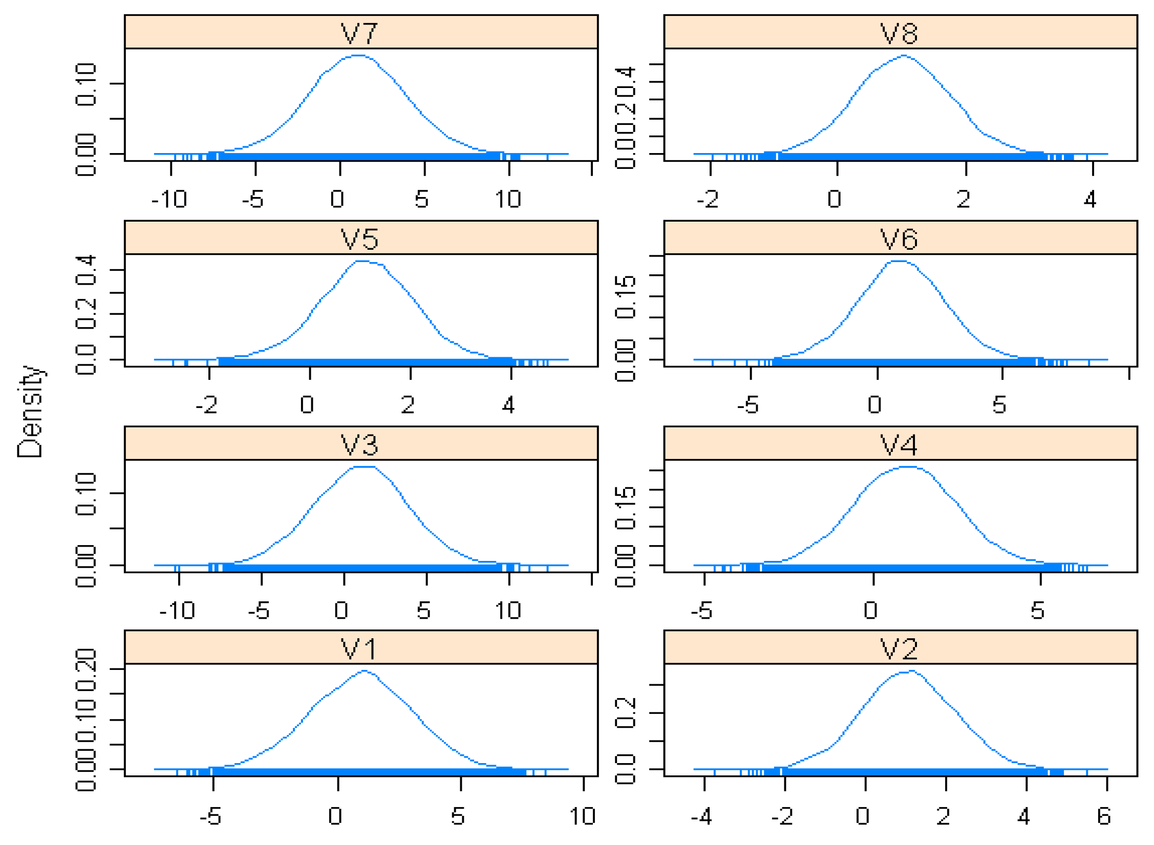
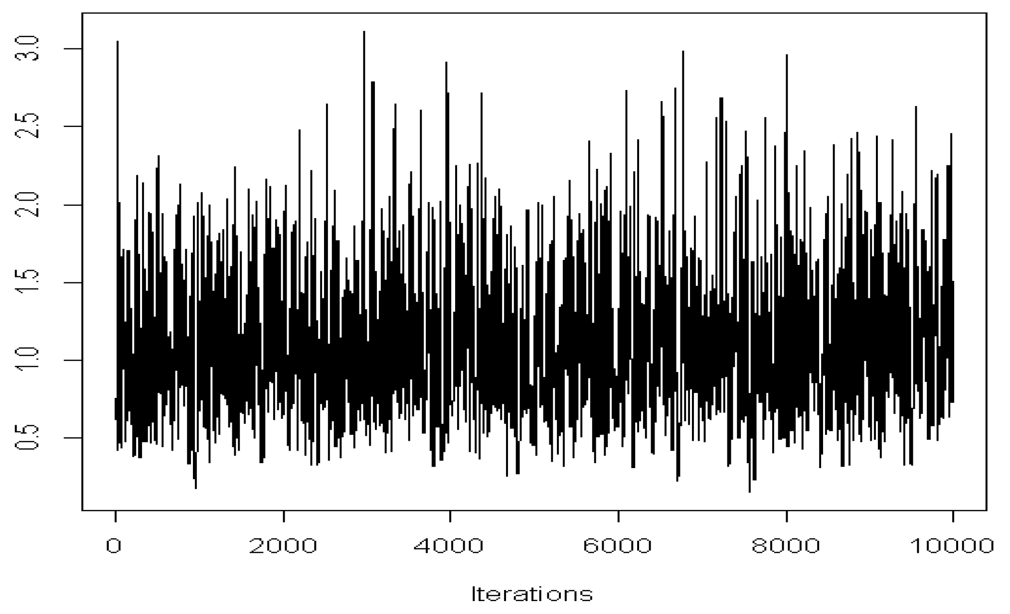
4.1.1. Estimation of Parameters

The parameters for the HBLD model, which were estimated using the simulated data $({\tilde{\theta }}_1, \dots , {\tilde{\theta }}_{30})$, are given in Table 1. It is expected that the estimated values would be close to the true values. The Gibbs sampler formulation is used to approximate the joint posterior distribution of parameters for the HBLD model. A cycle of 50,000 iterations is executed, but only the last 10,000 iterations are of use in determining the convergence of the chains of parameters.

The Geweke test [31], the Heidelberger and Welch test (H–W) [32], and the Raftery and Lewis test (R–L) [33] are the diagnostic tests used to determine whether the chains of parameters in the HBLD model have converged. The results of the MCMC convergence diagnostics using CODA and the values of the estimated parameters are presented in

Table 2. The MCMC convergence diagnostics for ${\tau }^2$, ${\beta }_0,\dots ,{\beta }_7$ using the Geweke, H–W, and R–L tests (the simulated effect sizes).

Test Variable	Geweke	H–W	R–L
${\tau }^2$	z-score −0.348	Stationarity test: passed p-value: 0.867 Half-width test: passed Half-width: 0.021	Dependence factor (I) 1.49
${\beta }_0$	z-score −0.2721	Stationarity test: passed p-value: 0.8316 Half-width test: passed Half-width: 0.0641	Dependence factor (I) 1.28
${\beta }_1$	z-score −1.0362	Stationarity test: passed p-value: 0.3383 Half-width test: passed Half-width: 0.0486	Dependence factor (I) 1.65
${\beta }_2$	z-score −1.0351	Stationarity test: passed p-value: 0.0643 Half-width test: passed Half-width: 0.0706	Dependence factor (I) 1.08
${\beta }_3$	z-score −0.4734	Stationarity test: passed p-value: 0.1425 Half-width test: passed Half-width: 0.0623	Dependence factor (I) 1.77
${\beta }_4$	z-score 0.5459	Stationarity test: passed p-value: 0.5384 Half-width test: passed Half-width: 0.0391	Dependence factor (I) 1.68
${\beta }_5$	z-score 0.5796	Stationarity test: passed p-value: 0.5736 Half-width test: passed Half-width: 0.0744	Dependence factor (I) 2.56
${\beta }_6$	z-score −0.5616	Stationarity test: passed p-value: 0.5231 Half-width test: passed Half-width: 0.0751	Dependence factor (I) 1.08
${\beta }_7$	z-score −0.7367	Stationarity test: passed p-value: 0.7495 Half-width test: passed Half-width: 0.0352	Dependence factor (I) 2.84

.

The z-score for ${\tau }^2$ is −0.348 for the Geweke test. As this value is between −2 and 2, it could be concluded that the chains of parameters have reached convergence at a 5% significance level. The stationarity test for ${\tau }^2$ is passed with a p-value of 0.867 for the H–W diagnostic test, under the null hypothesis that the MCMC chain is stationary. Furthermore, the half-width test is passed as the ratio between the half-width and the mean is lower than eps = 0.1 for the H–W test. This also suggested that the chains of parameters have reached convergence. The R–L test shows that the dependence factor (I) for ${\tau }^2$ is lower than 5.0, indicating that the sample is less correlated, confirming the convergence. The z-scores for ${\beta }_0,\dots ,{\beta }_7$ are all between −2 and 2 for the Geweke diagnostic test. The stationarity tests for ${\beta }_0,\dots ,{\beta }_7$ are passed with p-values greater than 0.05, suggesting that the null hypothesis of being stationary is not rejected for each parameter. The half-width tests of all parameters are passed as their values are less than the product of eps (0.1) with the corresponding sample mean for each parameter. The dependence factors (I) for the R–L diagnostic test are all below 5.0, which suggests that the sample is less correlated. All of these results together suggest that the chains of parameters have converged.

4.1.2. Estimation Results

Having confirmed the convergence of MCMC, the estimated values of ${\tau }^2$, ${\beta }_0,\dots ,{\beta }_7$ and ${\theta }_1^{\prime }$, …, ${\theta }_{30}^{\prime },$ together with corresponding 95% credible intervals (CI) and standard deviations (SD) are presented below. This data will be used to draw conclusions about the parameters for the model.

Table 3. Estimated parameters for the HBLD model using the Gibbs sampler algorithm (simulated data).

True Value	$\mathbf{Estimated} \mathbf{Value} \mathbf{of} {\tau }^2\mathbf{with} \mathbf{the} 95\% \mathbf{CI} \mathbf{and} \mathbf{SD}$
${\tau }^2$ = 1.2	${\widehat{\tau }}^2$ = 1.17 with (0.4911, 2.4756) and 0.5304
	Estimated value of ${\beta }_0, \dots , {\beta }_7$ with the 95% CI and SD
	Parameter estimates	95 % CI	SD
${\beta }_0$ = 1.0275	${\widehat{\beta }}_0$ = 0.9488	(−3.0529, 5.086)	2.0928
${\beta }_1$ = 0.9212	${\widehat{\beta }}_1$ = 1.0829	(−1.3224, 3.461)	1.2063
${\beta }_2$ = 0.8836	${\widehat{\beta }}_2 =$1.0041	(−4.7594, 6.696)	2.9126
${\beta }_3$ = 1.0701	${\widehat{\beta }}_3 =$1.0365	(−1.8536, 3.911)	1.4685
${\beta }_4$ = 1.1283	${\widehat{\beta }}_4$ = 1.1428	(−0.6644, 2.947)	0.9185
${\beta }_5$ = 1.0231	${\widehat{\beta }}_5$ = 1.0100	(−2.4272, 4.338)	1.7186
${\beta }_6$ = 0.8390	${\widehat{\beta }}_6$ = 1.0321	(−4.6317, 6.568)	2.8615
${\beta }_7$ = 1.0911	${\widehat{\beta }}_7 =$1.0252	(−0.4668, 2.517)	0.7603
${\theta }_1^{\prime }$, …, ${\theta }_{30}^{\prime }$	Estimated value of ${\theta }_1^{\prime }, \dots , {\theta }_{30}^{\prime }$ with the 95% CI and SD
${\theta }_1^{\prime }$ = 4.3449	${\widehat{\theta }}_1^{\prime }$ = 4.349	(2.145, 6.535)	1.1095
${\theta }_2^{\prime }$ = 6.1647	${\widehat{\theta }}_2^{\prime }$ = 6.081	(3.563, 8.586)	1.2684
${\theta }_3^{\prime }$ = 4.3748	${\widehat{\theta }}_3^{\prime }$ = 4.385	(2.491, 6.223)	0.9371
${\tilde{\theta }}_4 =$4.8439	${\widehat{\theta }}_4^{\prime } =$4. 864	(3.012, 6.739)	0.9396
${\theta }_5^{\prime }$ = 8.5522	${\widehat{\theta }}_5^{\prime }$ = 8.641	(6.578, 10.646)	1.0190
${\theta }_6^{\prime }$ = 8.6170	${\widehat{\theta }}_6^{\prime }$ = 8.641	(7.221, 10.046)	0.7154
${\theta }_7^{\prime }$ = 7.6657	${\widehat{\theta }}_7^{\prime }$ = 7.624	(5.763, 9.500)	0.9375
${\theta }_8^{\prime }$ = 4.4449	${\widehat{\theta }}_8^{\prime }$ = 4.453	(2.000, 6.997)	1.2566
${\theta }_9^{\prime }$ = 6.8181	${\widehat{\theta }}_9^{\prime }$ = 6.754	(3.823, 9.767)	1.5146
${\theta }_{10}^{\prime }$ = 5.0117	${\widehat{\theta }}_{10}^{\prime }$ = 5.050	(2.739, 7.391)	1.1675
${\theta }_{11}^{\prime }$ = 5.1228	${\widehat{\theta }}_{11}^{\prime }$ = 5.170	(3.609, 6.710)	0.7923
${\theta }_{12}^{\prime }$ = 6.9209	${\widehat{\theta }}_{12}^{\prime }$ = 6.948	(5.237, 8.691)	0.8780
${\theta }_{13}^{\prime }$ = 4.3826	${\widehat{\theta }}_{13}^{\prime }$ = 4.416	(2.316, 6.545)	1.0711
${\theta }_{14}^{\prime }$ = 4.8544	${\widehat{\theta }}_{14}^{\prime }$ = 4.816	(2.480, 7.086)	1.1663
${\theta }_{15 }^{\prime }$ = 8.0901	${\widehat{\theta }}_{15}^{\prime }$ = 8.004	(5.467, 10.610)	1.2948
${\theta }_{16 }^{\prime }$ = 7.9717	${\widehat{\theta }}_{16}^{\prime }$ = 7.895	(5.233, 10.560)	1.3355
${\theta }_{17}^{\prime }$ = 7.7095	${\widehat{\theta }}_{17}^{\prime }$ = 7.655	(5.507, 9.779)	1.0880
${\theta }_{18}^{\prime }$ = 4.3726	${\widehat{\theta }}_{18}^{\prime }$ = 4.362	(2.355, 6.352)	1.0209
${\theta }_{19}^{\prime }$ = 5.0682	${\widehat{\theta }}_{19}^{\prime }$ = 5.105	(3.413, 6.857)	0.8603
${\theta }_{20 }^{\prime }$ = 4.9958	${\widehat{\theta }}_{20}^{\prime }$ = 5.046	(3.191, 6.888)	0.9230
${\theta }_{21}^{\prime }$ = 4.4190	${\widehat{\theta }}_{21}^{\prime }$ = 4.396	(3.105, 5.717)	0.6644
${\theta }_{22}^{\prime }$ = 4.3480	${\widehat{\theta }}_{22}^{\prime }$ = 4.388	(2.714, 6.050)	0.8451
${\theta }_{23}^{\prime }$ = 4.3539	${\widehat{\theta }}_{23}^{\prime }$ = 4.367	(2.161, 6.559)	1.1104
${\theta }_{24 }^{\prime }$ = 4.8056	${\widehat{\theta }}_{24}^{\prime }$ = 4.875	(2.543, 7.324)	1.1895
${\theta }_{25 }^{\prime }$ = 8.6786	${\widehat{\theta }}_{25}^{\prime }$ = 8.621	(6.908,10.327)	0.8661
${\theta }_{26 }^{\prime }$ = 8.6407	${\widehat{\theta }}_{26}^{\prime }$ = 8.614	(7.219, 9.975)	0.7026
${\theta }_{27}^{\prime }$ = 7.6830	${\widehat{\theta }}_{27}^{\prime }$ = 7.634	(6.102, 9.158)	0.7738
${\theta }_{28 }^{\prime }$ = 4.4835	${\widehat{\theta }}_{28}^{\prime }$ = 4.480	(1.850, 7.127)	1.3389
${\theta }_{29}^{\prime }$ = 5.0045	${\widehat{\theta }}_{29}^{\prime }$ = 5.033	(3.023, 7.089)	1.0234
${\theta }_{30}^{\prime }$ = 5.0403	${\widehat{\theta }}_{30}^{\prime }$ = 5.017	(3.610, 6.440)	0.7170

shows the results of parameter estimates obtained using the Gibbs sampler algorithm under the assumption of a dependence structure on the model.

As can be seen from Table 3, the estimated value of ${\tau }^2$ is close to the true value. This indicates that the point estimate for ${\tau }^2$ is consistent. Moreover, from the first and second columns of Table 3, the estimated values of some parameters ${\beta }^{\prime }s$ are not very close to the true values. Some standard deviations are quite large compared to their point estimates. This indicated that the data is spread out over a large range of values. However, all of the estimated values of $\beta s$ and their corresponding true values lay within their credible interval. This indicated that 95% of the true value will lie within the range. For example, the estimated value of ${\tau }^2$ is 1.17, associated with the 95% CI (0.4911, 2.4756). This is close to the true value of ${\tau }^2$ (1.2). The estimated value of the intercept (${\widehat{\beta }}_0$) is 0.9488, associated with its 95% CI (−3.0529, 5.086). This shows that the true value of the intercept, ${\beta }_0$ (1.0275), lay within the 95% credible interval of ${\widehat{\beta }}_0$. From Table 3, the CIs for the estimated parameter $\beta s$ all include zero, which suggests that there is no significant difference between the means of the two covariates which is fixed in the simulation study.

The marginal posterior densities of ${\beta }_0$, ${\beta }_1$, ${\beta }_2$, ${\beta }_3$, ${\beta }_4$, ${\beta }_5$, ${\beta }_6$, and ${\beta }_7$, which are shown in Figure 1 and labelled V1, V2, V3, V4, V5, V6, V7, and V8, respectively, are unimodal and symmetric. Figure 2 displays the trace plots of ${\beta }_0,\dots ,{\beta }_7$. These figures show that the final 10,000 iterations for the chains of parameters are relatively stable with very small fluctuations only, confirming convergence.

Figure 3 shows that the density of ${\tau }^2$ is right-skewed with a mean value of 1.17 as ${\tau }^2$ is an inverse gamma distribution. The trace plot of ${\tau }^2$ is displayed in Figure 4. This figure shows that the chains of ${\tau }^2$ mixed relatively well with small fluctuations, confirming the convergence.

4.2. Case Study: Application of the HBLD Model to the Native Language Vocabulary Data

The HBLD model is applied to data obtained by [5]. The parameters for the models are approximated using the algorithm formulas given in Section 3.2. The dependence assumption is imposed on the variance–covariance matrix, $V$, at the sampling level of the model due to the use of the same data by two or more studies. A similar code to that used to estimate the parameters for the simulated data in Section 4.1 is executed. The results obtained using the Gibbs sampler algorithm are compared to the results obtained by [5] in order to assess the consistency of the parameters. The effect size of each study is calculated using the formula given by [5]. A dependence assumption is imposed at the sampling level of the model. This causes several off-diagonal entries of the variance–covariance matrix $V$ to be non-zero.

4.2.1. Estimation of Parameters

A total of 50,000 iterations are executed, but only the last 10,000 iterations are used to determine the convergence of parameters. The MCMC convergence diagnostics using CODA are performed to test for the convergence of each parameter. A side by side comparison of the values of the intercept $\left({\beta }_0\right)$ and ${\tau }^2$ obtained using the Gibbs sampler algorithm with the results obtained by [5] can be made using

Table 4. MCMC convergence diagnostics for values of ${\tau }^2$, ${\beta }_0,\dots ,{\beta }_5$ obtained by using the Gibbs sampler algorithm. Tests used included Geweke, H–W, and R–L tests.

Test Variable	Geweke	H-W	R-L
${\tau }^2$	z-score −1.527	Stationarity test: passed p-value: 0.204 Half-width test: passed Half-width: 0.0086	Dependence factor (I) 3.4
${\beta }_0$	z-score 0.2917	Stationarity test: passed p-value: 0.483 Half-width test: passed Half-width: 0.0012	Dependence factor (I) 1.23
${\beta }_1$	z-score −0.2912	Stationarity test: passed p-value: 0.834 Half-width test: passed Half-width: 0.0066	Dependence factor (I) 1.14
${\beta }_2$	z-score −0.8820	Stationarity test: passed p-value: 0.465 Half-width test: passed Half-width: 0.0039	Dependence factor (I) 2.21
${\beta }_3$	z-score −0.3594	Stationarity test: passed p-value: 0.720 Half-width test: passed Half-width: 0.0048	Dependence factor (I) 1.21
${\beta }_4$	z-score 0.1667	Stationarity test: passed p-value: 0.804 Half-width test: passed Half-width: 0.0034	Dependence factor (I) 1.17
${\beta }_5$	z-score −0.3995	Stationarity test: passed p-value: 0.769 Half-width test: passed Half-width: 0.0047	Dependence factor (I) 1.18

.

In this section, the convergence diagnostic tests for ${\tau }^2$, ${\beta }_0,\dots ,{\beta }_5$ are presented. This is followed by the estimation results for the parameters. ${\beta }_0$, the intercept parameter, is referred to as the estimation of the population mean effect size. The estimation of this parameter of interest is the primary objective of this case study.

The Geweke, H–W, and R–L tests are the MCMC diagnostic tests performed to determine the convergence of the parameters. The results of these tests of convergence for the parameters are given in Table 4 and are used to conclude whether the parameters achieved convergence.

Table 4 shows that the z-score of ${\tau }^2$ is −1.527. As this value lay between −2 and 2, it could be concluded that ${\tau }^2$ has reached convergence. The p-value of ${\tau }^2$ is 0.42. This confirms that the null hypothesis of ${\tau }^2$ is not rejected. The stationarity and half-width tests are passed for the H–W diagnostic. The dependence factor (I) for the R–L test is 3.4 lower than 5, indicating less correlated samples. It is likely that the convergence of the chains for ${\tau }^2$ has been achieved. The z-scores of parameters (${\beta }_0,\dots ,{\beta }_5$) are between −2 and 2 for the Geweke diagnostic tests, confirming that the chains of parameters reached convergence at a 5% significance level. The p-value of the $\beta s$ are less than 0.95, indicating that the null hypothesis is not rejected. Moreover, the stationarity tests for all parameters are passed after discarding 50% of the chains. The half-width tests are also passed. The dependence factors (I) of all variables are lower than 5 for the R–L diagnostic test, suggesting that the sample is less correlated. Together, all of these diagnostic tests indicate that the chains for ${\beta }_0,\dots ,{\beta }_5$ have converged.

4.2.2. Estimation Results

The parameter estimates for ${\tau }^2 {\beta }_0,\dots ,{\beta }_5$, and their associated credible intervals and standard deviations are presented in

Table 5. Parameter estimates for the HBLD model using the Gibbs sampler for the case study.

$\mathbf{Estimate} \mathbf{Result} \mathbf{of} {\tau }^2 \mathbf{with} \mathbf{the} 95\% \mathbf{CI} \mathbf{and} \mathbf{SD}$
${\widehat{\tau }}^2$ = 0.3106, CI (0.0764, 0.8201), SD = 0.207 (Gibbs sampler) ${\widehat{\tau }}^2$ = 0.3054, CI (−0.0643, 0.6750), SD = 0.1848 ([5])
Estimates results of ${\beta }_0,\dots , {\beta }_5$ with the 95% CI and SD
Parameter estimates	95 % CI	SD
${\widehat{\beta }}_0$ = 0.5756 (G-S) ${\widehat{\beta }}_0$ = 0.5769 ([5])	(0.4037, 0.7444) (G-S) (0.2659, 0.8879) (Stevens [5])	0.0866 (G-S) 0.1555 ([5])
${\widehat{\beta }}_1$ = −0.9469	(−1.9459, 0.1328)	0.5264
${\widehat{\beta }}_2=$−0.2432	(−0.7733, 0.2608)	0.2623
${\widehat{\beta }}_3=$0.2985	(−0.3606, 0.9554)	0.3347
${\widehat{\beta }}_4$ = 0.3710	(−0.1175, 0.8474)	0.2442
${\widehat{\beta }}_5$ = 0.5545	(−0.0827, 1.2247)	0.3329

. The point estimate of ${\tau }^2$ obtained by [5] is 0.3054, associated with a 95% credible interval of (−0.0643, 0.6750). This is relatively close to the value obtained using the Gibbs sampler algorithm (0.3106), and its 95% credible interval (0.0764, 0.8201). The width of the credible interval given by [5] is 0.7393. This is similar to the credible interval obtained using the Gibbs sampler algorithm (0.7437). The credible interval for ${\tau }^2$ obtained by [5] includes zero. This indicates that there is no significant difference between the means of the effect sizes ${\theta }^{\prime }$ in the data set. Moreover, the credible interval for ${\tau }^2$ obtained by the use of the Gibbs sampler does not include zero. This is reasonable because ${\tau }^2$ has an inverse gamma distribution whose scale is greater than zero. The standard deviation for ${\tau }^2$ obtained by [5] is 0.1848, which is smaller than the standard deviation obtained using the Gibbs sampler (0.207). This shows that Stevens and Taylor’s data is less spread out and more precise.

The point estimate of the intercepts (${\beta }_0$) obtained using the Gibbs sampler algorithm is similar to the result obtained by [5]. However, its credible interval is narrower than Steven’s results. This indicates that the more precise results are obtained for the population mean effect size (intercepts) when the Gibbs sampler algorithm is applied. From the application of the model to the data, it could be concluded that (${\beta }_0$ = 58%) the native-language vocabulary aids are effective as second language reading comprehension aids. From Table 5, the CIs for estimated parameters ${\beta }_1,\dots ,{\beta }_5$ are wider and all included the null value of a difference of 0%. We will not exclude the possibility that the covariates have any effect on the native-language (L1) vocabulary aids on second-language (L2) reading comprehension.

The density plot displayed in Figure 5a shows that the marginal posterior density of ${\beta }_0$ (intercept) is symmetric. This indicates that ${\beta }_0$ is normally distributed. Moreover, the trace plot displayed in panel (b) of Figure 5 shows that the last 10,000 iterations in the estimation of ${\beta }_0$ have relatively good mixing, suggesting that the chains have converged.

Figure 6 shows that the density plot of ${\tau }^2$ (panel a) is a right-skewed distribution. This potentially occurs since the conditional posterior distribution of ${\tau }^2$ is the inverse gamma distribution. In addition, the trace plot of ${\tau }^2$ (panel b) does not show good mixing. This suggests that the chains converged slowly.

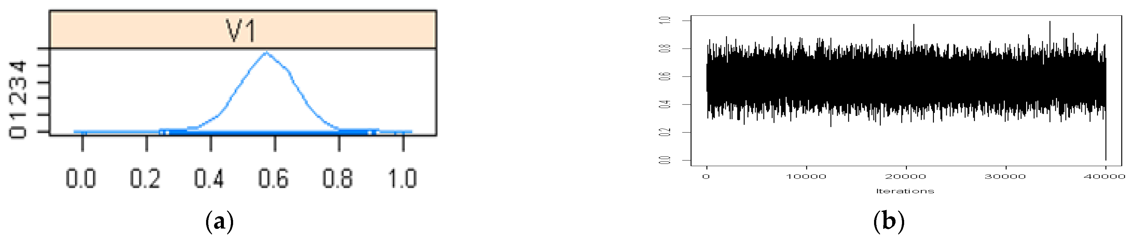
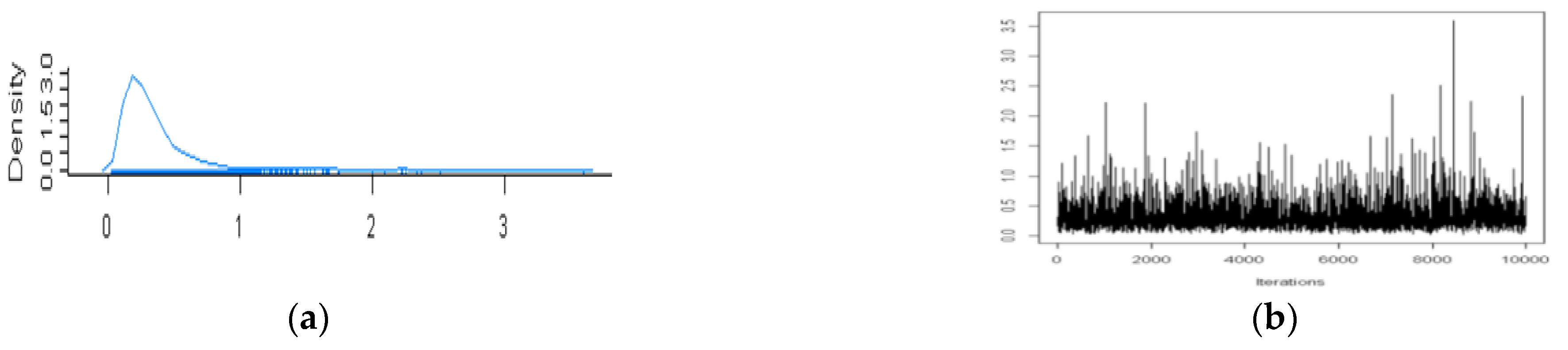
5. Prior Sensitivity Analysis

The sensitivity analysis of the HBLD model is conducted by changing the prior distribution of the model. The inverse gamma distribution on the variance of the model will be replaced using the log-logistic distribution.

5.1. Sensitivity Analysis of the HBLD Model

The authors of [34,35] stated that the results obtained using Bayesian models are potentially sensitive to the choice of prior distributions and hence a sensitivity analysis should always be performed to assess the robustness of models. This section presents an estimation of parameters for the HBLD model obtained using a different prior distribution on the variance component (${\tau }^2$) of the effect size (${\theta }^{\prime }$) for the model. The use of a different prior distribution allowed an assessment of the sensitivity of the model. One possible prior distribution that can be placed on ${\tau }^2$ is the log-logistic distribution [5,35].

Rewriting (1) using the log-logistic distribution as the prior ${\tau }^2$ gives:

$$\tilde{\theta }\sim MVN\left({\theta }^{\prime },V\right)$$

$$\epsilon \sim N \left(0, V\right)$$

$${\theta }^{\prime }\sim MVN \left(X\beta ,{\tau }^{2}I\right)$$

$${\delta }^2\sim N\left(0,{\tau }^{2}I\right)$$

$$\beta \sim MVN \left(b,D\right)$$

$${\tau }^2 \sim \mathrm{log-logistic} (c_0,\gamma )$$

(17)

where $c_0$ and $\gamma$ are the median and shape of ${\tau }^2,$ respectively. In Equation (17), the log-logistic distribution used for $p\left({\tau }^2\right)$ is defined by:

$$P\left({\tau }^2\right)=\frac{c_0}{{(c_0+{\tau }^2)}^2}, {\tau }^2 > 0$$

(18)

where $c_0=\sqrt{\frac{N}{tr\left\{{\left[\mathrm{diag}\left(\mathrm{V}\right)\right]}^{-1}\right\}}}$, N is the number of studies (or sub-studies) and $\gamma =1$.

This particular selection was used by [36] and [5]. Using (3)–(5) and (18), it can be seen that the joint posterior distribution of all parameters for the current HBLD model is given by:

$$P({\theta }^{\prime }, \beta , {\tau }^2 \left|{\tilde{\theta }}_{\left(l\right)})\right.={\left(2\pi \right)}^{-\frac{n}{2}}{\left|V_{\left(l\right)}\right|}^{-\frac{1}{2}}exp\left\{-\frac{1}{2}{\left({\tilde{\theta }}_{\left(l\right)}-{\theta }^{\prime }\right)}^T{V}_{\left(l\right)}^{-1}\left({\tilde{\theta }}_{\left(l\right)}-{\theta }^{\prime }\right)\right\}$$

$$\times {\left(2\pi \right)}^{-\frac{n}{2}}{\left|{\tau }^{2}I\right|}^{-\frac{1}{2}}exp\left\{-\frac{1}{2}{\left({\theta }^{\prime }-X\beta \right)}^T{\left({\tau }^{2}I\right)}^{-1}\left({\theta }^{\prime }-X\beta \right)\right\}$$

$$\times {\left(2\pi \right)}^{-\frac{p}{2}}{\left|D\right|}^{-\frac{1}{2}}exp\left\{-\frac{1}{2}{\left(\beta -b\right)}^T{D}^{-1}\left(\beta -b\right)\right\}$$

$$\times \frac{c_0}{{(c_0+{\tau }^2)}^2}$$

(19)

Using Equation (19), the conditional posterior distributions of ${\theta }^{\prime },$ given $\beta$ and ${\tau }^2$, $f({\theta }^{\prime }\left|\beta \right.,{\tau }^2),$ and $\beta ,$ given ${\theta }^{\prime }$ and ${\tau }^2$, $f(\beta \left|{\theta }^{\prime },{\tau }^2)\right.$, are obtained using a similar mathematical procedure to the one presented in Section 4.1. This approach allows the Gibbs sampler to be used to approximate $f({\theta }^{\prime }\left|\beta \right.,{\tau }^2)$ and $f(\beta \left|{\theta }^{\prime },{\tau }^2)\right.$ by iteratively sampling from the full conditional distributions, as given in Equations (8) and (16). Unfortunately, the conditional posterior distribution for ${\tau }^2$ could not be simplified for this model. This is due to the fact that the product of the prior distributions of $p(\beta \left|{\tau }^2)\right.$ and $p\left({\tau }^2\right)$ is in a non-standard form. This suggests that it is not possible to apply the Gibbs sampler algorithm to estimate ${\tau }^2$.

The authors of [11,28] stated that for complex models, conditional distributions are often available for some parameters, but not for others. In this situation, a combination of the Gibbs sampler and Metropolis–Hastings algorithms offers an alternative approach that can be used to generate a Markov Chain for the estimation of the joint posterior distribution of all parameters for the models. More generally, [12] stated that when the conditional posterior distributions of parameters are in non-standard form, it is enough to sample each full conditional by using a Metropolis–Hastings step. This approach is known as Metropolis within Gibbs, or, alternatively, as single-component Metropolis–Hastings sampling [11].

5.1.1. Posterior Analysis of the HBLD Model Using Metropolis within Gibbs

The Metropolis within Gibbs [11,12] is used to approximate the joint posterior distribution of all parameters for the HBLD model given in Equation (19). The Gibbs sampler has already been used to approximate $f({\theta }^{\prime }\left|\beta ,{\tau }^2\right.)$ and $f\left(\beta \left|{\theta }^{\prime },{\tau }^2\right.\right)$ (see the conditional posterior of ${\theta }^{\prime }$ given $\beta$ and $\tau$ and conditional posterior of $\beta$ given ${\theta }^{\prime }$ and ${\tau }^2$). This section describes the use of the Metropolis–Hastings algorithm to estimate ${\tau }^2$, $f\left({\tau }^2 \left|{\theta }^{\prime },\right. \beta \right)$.

Similar steps to those used with the Gibbs sampler algorithm (steps 1, 2, and 3 but not 4), are used to approximate the joint posterior distribution of all parameters for the HBLD model given in (19), as follows:

Steps 1, 2, and 3 are similar to the steps given in Section 3.2.

Step 4:

${{\tau }^2}^{\left(j\right)}$ given ${\theta }_1^{\prime \left(j\right)},\dots ,{\theta }_n^{\prime \left(j\right)},{\beta }_0^{\left(j\right)},\dots ,{\beta }_{p-1}^{\left(j\right)}$ is generated using the Metropolis–Hastings algorithm by implementing the following steps:

(a)

It is proposed that ${{\tau }^2}^{\ast }$ ~Gamma ($\delta +{{\tau }^2}^{\left(j-1\right)},\omega +{{\tau }^2}^{\left(j-1\right)}$).

The proposed distribution for ${{\tau }^2}^{\ast }$ is:

$$J_{\tau }\left({{\tau }^2}^{\ast }\right)= \frac{1}{{\left(\omega +{{\tau }^2}^{\left(j-1\right)}\right)}^{\left(\delta {+}^2{\tau }^{\left(j-1\right)}\right)}/\left(\delta +{{\tau }^2}^{\left(j-1\right)}\right)}{\left({{\tau }^2}^{\ast }\right)}^{\left(\delta +{{\tau }^2}^{\left(j-1\right)}-1\right)}exp\left(-\frac{{{\tau }^2}^{\ast }}{\omega +{{\tau }^2}^{\left(j-1\right)}}\right),$$

(20)

where $\delta +{{\tau }^2}^{\left(j-1\right)}$ > 0 and $\omega +{{\tau }^2}^{\left(j-1\right)}$ > 0 are shape and scale, respectively, and ${{\tau }^2}^{\ast }$ ϵ (0, ∞).

(b)

The acceptance ratio for the parameter ${\tau }^2$ is as follows:

$$r_{\tau }=\frac{P\left({\theta }^{\prime \left(j\right)},{\beta }^{\left(j\right)}{{\tau }^2}^{\ast }|{\tilde{\theta }}_{\left(l\right)}\right)}{P\left({\theta }^{\prime \left(j\right)},{\beta }^{\left(j\right)},{2\tau }^{\left(j-1\right)}|{\tilde{\theta }}_{\left(l\right)}\right)} \times \frac{J_{\tau }\left({{\tau }^2}^{\left(j-1\right)}\right)}{J_{\tau }\left({{\tau }^2}^{\ast }\right)}$$

$$r_{\tau }\propto \frac{{\left(2\pi \right)}^{-\frac{n}{2}}{\left|{\tau }^{2\ast }I\right|}^{-\frac{1}{2}}exp\left\{-\frac{1}{2}{\left({\theta }^{\prime \left(j\right)}-X{\beta }^{\left(j\right)}\right)}^T{\left({\tau }^{2\ast }I\right)}^{-1}\left({\theta }^{\prime \left(j\right)}-X{\beta }^{\left(j\right)}\right)\right\}}{{\left(2\pi \right)}^{-\frac{n}{2}}{\left|{\tau }^{2\left(j-1\right)}I\right|}^{-\frac{1}{2}}exp\left\{-\frac{1}{2}{\left({\theta }^{\prime \left(j\right)}-X{\beta }^{\left(j\right)}\right)}^T{\left({\tau }^{2\left(j-1\right)}I\right)}^{-1}\left({\theta }^{\prime \left(j\right)}-X{\beta }^{\left(j\right)}\right)\right\}}$$

$$\times \frac{\frac{c_0}{{\left(c_0+{{\tau }^2}^{\ast }\right)}^2}}{\frac{c_0}{{\left(c_0+{{\tau }^2}^{\left(j-1\right)}\right)}^2}}\times \frac{\frac{1}{{\left({\omega +{\tau }^2}^{\left(j-1\right)}\right)}^{\left(\delta +{{\tau }^2}^{\left(j-1\right)}\right)}\Gamma \left(\delta +{{\tau }^2}^{\left(j-1\right)}\right)}{\left({{\tau }^2}^{\left(j-1\right)}\right)}^{\left(\delta +{{\tau }^2}^{\left(j-1\right)}-1\right)}exp\left(-\frac{{{\tau }^2}^{\left(j-1\right)}}{{\omega +{\tau }^2}^{\left(j-1\right)}}\right)}{\frac{1}{{\left({\omega +{\tau }^2}^{\left(j-1\right)}\right)}^{\left(\delta +{{\tau }^2}^{\left(j-1\right)}\right)}\Gamma \left(\delta +{{\tau }^2}^{\left(j-1\right)}\right)}{\left({{\tau }^2}^{\ast }\right)}^{\left(\delta +{{\tau }^2}^{\left(j-1\right)}-1\right)}exp\left(-\frac{{{\tau }^2}^{\ast }}{{\omega +{\tau }^2}^{\left(j-1\right)}}\right)}$$

$$r_{\tau }=\frac{{\left(2\pi \right)}^{-\frac{n}{2}}{\left|{\tau }^{2\ast }I\right|}^{-\frac{1}{2}}exp \left\{-\frac{1}{2}{\left({\theta }^{\prime \left(j\right)}-X{\beta }^{\left(j\right)}\right)}^T{\left({\tau }^{2\ast }I\right)}^{-1}\left({\theta }^{\prime \left(j\right)}-X{\beta }^{\left(j\right)}\right)\right\}}{{\left(2\pi \right)}^{-\frac{n}{2}}{\left|{\tau }^{2\left(j-1\right)}I\right|}^{-\frac{1}{2}}exp \left\{-\frac{1}{2}{\left({\theta }^{\prime \left(j\right)}-X{\beta }^{\left(j\right)}\right)}^T{\left({\tau }^{2\left(j-1\right)}I\right)}^{-1}\left({\theta }^{\prime \left(j\right)}-X{\beta }^{\left(j\right)}\right)\right\}} \times \frac{\frac{c_0}{{\left(c_0+{\tau }^{2\ast }\right)}^2}}{\frac{c_0}{{\left(c_0+{\tau }^{2\left(j-1\right)}\right)}^2}}$$

$$\times \frac{{\left({{\tau }^2}^{\left(j-1\right)}\right)}^{\left(\delta +{\tau }^{2\left(j-1\right)}-1\right)}exp\left(-\frac{{{\tau }^2}^{\left(j-1\right)}}{\omega +{\tau }^{2\left(j-1\right)}}\right)}{{\left({{\tau }^2}^{\ast }\right)}^{\left(\delta +{\tau }^{2\left(j-1\right)}-1\right)}exp\left(-\frac{{{\tau }^2}^{\ast }}{\omega +{\tau }^{2\left(j-1\right)}}\right)}$$

(21)

(c)

The parameter U is sampled from $U\sim \mathrm{Uniform} \left(0,1\right)$.

$$\mathrm{If} r_{\tau }>U, \mathrm{then} {{\tau }^2}^{\left(j\right)}={{\tau }^2}^{\ast } \mathrm{otherwise} {{\tau }^2}^{\left(j\right)}={{\tau }^2}^{\left(j-1\right)}.$$

Step 5. Steps 2, 3, and 4 are repeated until the chains reach convergence.

A sensitivity analysis is conducted using the simulated data given in Section 4.1. The proposed MCMC algorithm, namely the Metropolis within Gibbs algorithm as formulated above, is used to estimate the parameters for the current HBLD model. The estimates obtained using the Metropolis within Gibbs algorithm are compared to the results obtained using the Gibbs sampler algorithm to determine the sensitivity of the model when the prior distribution for ${\tau }^2$ is performed.

5.1.2. Estimation of Parameters

In order to determine the sensitivity of the model, the parameters are estimated using the simulated data ${\tilde{\theta }}_1,\dots ,{\tilde{\theta }}_{30}$, as presented in Table 1. The formulation obtained using the Metropolis within Gibbs algorithm for the HBLD model is used to estimate these parameters. A cycle of 60,000 iterations is executed, but the only last 10,000 iterations are used to determine the convergence of the parameters.

The results of the MCMC convergence diagnostics using CODA and the point estimates found for all parameters are discussed in

Table 6. The MCMC convergence diagnostics for ${\tau }^2$, ${\beta }_0,\dots ,{\beta }_7$ using the Geweke, H–W, and R–L tests (the simulated effect sizes) by using log-logistic distribution for ${\tau }^2$.

Test Variable	Geweke	H-W	R-L
${\tau }^2$	z-score −1.702	Stationarity test: passed p-value: 0.29 Half-width test: passed Half-width: 0.0275	Dependence factor (I) 26.9
${\beta }_0$	z-score −0.0771	Stationarity test: passed p-value: 0.479 Half-width test: passed Half-width: 0.0658	Dependence factor (I) 1.23
${\beta }_1$	z-score 0.4396	Stationarity test: passed p-value: 0.266 Half-width test: passed Half-width: 0.0492	Dependence factor (I) 2.92
${\beta }_2$	z-score 1.38061	Stationarity test: passed p-value: 0.968 Half-width test: passed Half-width: 0.0700	Dependence factor (I) 1.12
${\beta }_3$	z-score −0.9961	Stationarity test: passed p-value: 0.536 Half-width test: passed Half-width: 0.0701	Dependence factor (I) 2.96
${\beta }_4$	z-score −0.3347	Stationarity test: passed p-value: 0.469 Half-width test: passed Half-width: 0.0415	Dependence factor (I) 2.73
${\beta }_5$	z-score −0.5931	Stationarity test: passed p-value: 0.435 Half-width test: passed Half-width: 0.0708	Dependence factor (I) 1.64
${\beta }_6$	z-score 0.5017	Stationarity test: passed p-value: 0.488 Half-width test: passed Half-width: 0.0766	Dependence factor (I) 1.16
${\beta }_7$	z-score 0.2488	Stationarity test: passed p-value: 0.143 Half-width test: passed Half-width: 0.0356	Dependence factor (I) 2.63

.

The R–L diagnostic test shows that the dependence factor (I) for ${\tau }^2$ is higher than 5.0, indicating that the sample is highly correlated. However, the z-score for ${\tau }^2$ (−1.702) is between −2 to 2 for the Geweke test, confirming the convergence at a 5% significance level. The p-value of ${\tau }^2$ is 0.29 for the H–W diagnostic test, indicating that the null hypothesis of the MCMC chain is not rejected. The half-width test is also passed for the H–W test. This suggests that the chains of parameters have reached convergence. The z-scores for ${\beta }_0,\dots ,{\beta }_7$ are between −2 and 2 for the Geweke diagnostic tests. The stationarity tests for ${\beta }_0,\dots ,{\beta }_7$ are passed with p-values greater than 0.05, indicating that the null hypothesis of the MCMC chains being stationary is not rejected. The half-width tests of all parameters are passed as their values are less than the product of eps (0.1) with the corresponding sample mean for each parameter. The dependence factors (I) for the R–L diagnostic test are below 5.0, which indicates that the samples are less correlated. All of these results together confirm that the chains of parameters have converged.

5.1.3. Estimation Results

The estimated values of ${\tau }^2$, ${\beta }_0,\dots ,{\beta }_7$, and ${\theta }_1^{\prime }$, …, ${\theta }_{30}^{\prime }$, with their corresponding 95% credible intervals (CI) and standard deviations (SD), are given below. This data is used to describe conclusions about the parameters for the model.

Table 7. Estimated parameters for the HBLD model using the Metropolis within Gibbs algorithm (simulated data).

True Value	$\mathbf{Estimated} \mathbf{Value} \mathbf{of} {\tau }^2\mathbf{with} \mathbf{the} 95\% \mathbf{CI} \mathbf{and} \mathbf{SD}$
${\tau }^2$ = 1.2	${\widehat{\tau }}^2$ = 1.03 with (0.3366, 2.0239) and 0.4416
	Estimated value of ${\beta }_0, \dots , {\beta }_7$ with the 95% CI and SD
	Parameter estimates	95 % CI	SD
${\beta }_0$ = 1.0275	${\widehat{\beta }}_0$ = 0.9752	(−3.2394, 5.074)	2.1101
${\beta }_1$ = 0.9212	${\widehat{\beta }}_1$ = 1.0745	(−1.2130, 3.387)	1.1644
${\beta }_2$ = 0.8836	${\widehat{\beta }}_2 =$1.0145	(−4.5127, 6.652)	2.8453
${\beta }_3$ = 1.0701	${\widehat{\beta }}_3 =$0.9565	(−1.9272, 3.881)	1.4831
${\beta }_4$ = 1.1283	${\widehat{\beta }}_4$ = 1.1468	(−0.6747, 2.914)	0.9084
${\beta }_5$ = 1.0231	${\widehat{\beta }}_5$ = 0.9792	(−2.3408, 4.316)	1.6892
${\beta }_6$ = 0.8390	${\widehat{\beta }}_6$ = 1.0569	(−4.5968, 6.699)	2.8607
${\beta }_7$ = 1.0911	${\widehat{\beta }}_7 =$1.0242	(−0.3861, 2.477)	0.7322
${\theta }_1^{\prime }$, …, ${\theta }_{30}^{\prime }$	Estimated value of ${\theta }_1^{\prime } , \dots , {\theta }_{30}^{\prime }$ with the 95% CI and SD
${\theta }_1^{\prime }$ = 4.3449	${\widehat{\theta }}_1^{\prime }$ = 4.352	(2.330, 6.390)	1.0198
${\theta }_2^{\prime }$ = 6.1647	${\widehat{\theta }}_2^{\prime }$ = 6.088	(3.744, 8.465)	1.2088
${\theta }_3^{\prime }$ = 4.3748	${\widehat{\theta }}_3^{\prime }$ = 4.404	(2.634, 6.233)	0.8922
${\tilde{\theta }}_4 =$4.8439	${\widehat{\theta }}_4^{\prime }$ = 4. 834	(3.080, 6.598)	0.8933
${\theta }_5^{\prime }$ = 8.5522	${\widehat{\theta }}_5^{\prime }$ = 8.591	(6.633, 10.528)	1.9829
${\theta }_6^{\prime }$ = 8.6170	${\widehat{\theta }}_6^{\prime }$ = 8.628	(7.243, 9.985)	0.7009
${\theta }_7^{\prime }$ = 7.6657	${\widehat{\theta }}_7^{\prime }$ = 7.644	(5.842,9.400)	0.9081
${\theta }_8^{\prime }$ = 4.4449	${\widehat{\theta }}_8^{\prime }$ = 4.461	(2.073, 6.826)	1.1911
${\theta }_9^{\prime }$ = 6.8181	${\widehat{\theta }}_9^{\prime }$ = 6.742	(3.762, 9.671)	1.4920
${\theta }_{10}^{\prime }$ = 5.0117	${\widehat{\theta }}_{10}^{\prime }$ = 5.021	(2.895, 7.151)	1.0734
${\theta }_{11}^{\prime }$ = 5.1228	${\widehat{\theta }}_{11}^{\prime }$ = 5.159	(3.649, 6.688)	0.7769
${\theta }_{12}^{\prime }$ = 6.9209	${\widehat{\theta }}_{12}^{\prime }$ = 6.950	(5.280, 8.637)	0.8628
${\theta }_{13}^{\prime }$ = 4.3826	${\widehat{\theta }}_{13}^{\prime }$ = 4.407	(2.388, 6.413)	1.0017
${\theta }_{14}^{\prime }$ = 4.8544	${\widehat{\theta }}_{14}^{\prime }$ = 4.759	(2.567 6.922)	1.0826
${\theta }_{15 }^{\prime }$ = 8.0901	${\widehat{\theta }}_{15}^{\prime }$ = 8.003	(5.578, 10.464)	1.2199
${\theta }_{16 }^{\prime }$ = 7.9717	${\widehat{\theta }}_{16}^{\prime }$ = 7.865	(5.360, 10.309)	1.2489
${\theta }_{17}^{\prime }$ = 7.7095	${\widehat{\theta }}_{17}^{\prime }$ = 7.682	(5.671, 9.710)	1.0331
${\theta }_{18}^{\prime }$ = 4.3726	${\widehat{\theta }}_{18}^{\prime }$ = 4.361	(2.423, 6.267)	0.9815
${\theta }_{19}^{\prime }$ = 5.0682	${\widehat{\theta }}_{19}^{\prime }$ = 5.068	(3.473, 6.697)	0.8142
${\theta }_{20 }^{\prime }$ = 4.9958	${\widehat{\theta }}_{20}^{\prime }$ = 5.024	(3.243, 6.827)	0.8984
${\theta }_{21}^{\prime }$ = 4.4190	${\widehat{\theta }}_{21}^{\prime }$ = 4.383	(3.127, 5.644)	0.6412
${\theta }_{22}^{\prime }$ = 4.3480	${\widehat{\theta }}_{22}^{\prime }$ = 4.380	(2.802, 5.975)	0.8066
${\theta }_{23}^{\prime }$ = 4.3539	${\widehat{\theta }}_{23}^{\prime }$ = 4.358	(2.217, 6.440)	1.0441
${\theta }_{24 }^{\prime }$ = 4.8056	${\widehat{\theta }}_{24}^{\prime }$ = 4.824	(2.593, 7.017)	1.0996
${\theta }_{25 }^{\prime }$ = 8.6786	${\widehat{\theta }}_{25}^{\prime }$ = 8.629	(6.993,10.270)	0.8288
${\theta }_{26 }^{\prime }$ = 8.6407	${\widehat{\theta }}_{26}^{\prime }$ = 8.609	(7.258, 9.958)	0.6854
${\theta }_{27}^{\prime }$ = 7.6830	${\widehat{\theta }}_{27}^{\prime }$ = 7.645	(6.147, 9.132)	0.7550
${\theta }_{28 }^{\prime }$ = 4.4835	${\widehat{\theta }}_{28}^{\prime }$ = 4.459	(1.893, 6.928)	1.2707
${\theta }_{29}^{\prime }$ = 5.0045	${\widehat{\theta }}_{29}^{\prime }$ = 5.018	(3.117, 6.941)	0.9602
${\theta }_{30}^{\prime }$ = 5.0403	${\widehat{\theta }}_{30}^{\prime }$ = 5.008	(3.655, 6.379)	0.6928

shows the results of the parameter estimates obtained by using a log-logistic distribution for ${\tau }^2$ on the model.

As can be seen from Table 7, the estimated value of ${\tau }^2$ is 1.03, corresponding with its standard deviation (0.4416), which is close to the true values. This indicates that 95% of the true value will lie within the range. In the first and second columns of Table 7, the estimated values of some parameters $\beta s$ are not very close to the true values. Some standard deviations are quite big compared to their point estimates. This indicates that the data is spread out over a large range of values. However, all of the estimated values of $\beta s$ and their corresponding true values lay within their credible intervals, indicating the consistency of the parameters. For example, the estimated value of the intercept (${\widehat{\beta }}_0$) is 0.9752, associated with its 95% CI (−3.2394, 5.074). This shows that the true value of the intercept, ${\beta }_0$ (1.0275), lay within the 95% credible interval of ${\widehat{\beta }}_0$. From Table 7, the CI’s for estimated parameter $\beta s$ all include zero, which suggests that there is no significant difference between $\beta s$.

The marginal posterior densities of ${\beta }_0$, ${\beta }_1$, ${\beta }_2$, ${\beta }_3$, ${\beta }_4$, ${\beta }_5$, ${\beta }_6$, and ${\beta }_7$, which are shown in Figure 7 and labelled V1, V2, V3, V4, V5, V6, V7, and V8, respectively, are unimodal and symmetric. Figure 8 displays the trace plots of ${\beta }_0$, …, ${\beta }_7$. These figures show that the final 10,000 iterations for the chains of parameters were relatively stable with very small fluctuations only, confirming convergence.

Figure 9 shows that the density of ${\tau }^2$ is right-skewed with a mean value of 1.03 as ${\tau }^2$ is a log-logistic distribution. The trace plot of ${\tau }^2$ is displayed in Figure 10. This figure shows that the chains of ${\tau }^2$ mixed relatively well with small fluctuations, confirming the convergence. In addition, the acceptance rate for ${\tau }^2$ is 44%, indicating that the chain moves rapidly across the whole distribution without getting stuck in any one place.

Comparison values of the intercept (${\beta }_0$) and ${\tau }^2$ obtained by using different prior distributions for ${\tau }^2$ are shown in

Table 8. Comparison of parameter estimates ${\beta }_0$ (intercept) and ${\tau }^2$ between the use of the Gibbs sampler algorithm and the Metropolis within Gibbs (simulated data).

Parameters	True Value	Gibbs Sampler Algorithm (Inverse Gamma)		Metropolis within Gibbs (Log-Logistic)
		Mean with CI	SD	Mean with CI	SD
${\beta }_0$(intercept)	1.0275	0.9488 (−3.0529, 5.086)	2.09	0.9752 (−3.2394, 5.074)	2.11
${\tau }^2$	1.2	1.17 (0.4911, 2.4756)	0.53	1.03 (0.3366, 2.0239)	0.44

. The standard deviation for the intercept (${\beta }_0$) obtained by the use of the log-logistic distribution is similar to the standard deviation obtained by the use of the inverse gamma distribution (2.09). This indicates that the use of different prior distributions for ${\tau }^2$ on the model is insensitive to the intercept (${\beta }_0$). Furthermore, the standard deviation obtained by using the inverse gamma distribution for the parameter ${\tau }^2$ is 0.53 when the log-logistic distribution is smaller (0.44). The lower standard deviation obtained by the use of the log-logistic distribution indicates the precision of the estimated parameter. It can also be concluded that the parameter of ${\tau }^2$ is insensitive by the use of different prior distributions.

5.2. Application of the HBLD Model to the Native Language Vocabulary Data: Metropolis within Gibbs

The native language vocabulary data is applied for the HBLD model which is developed using the Metropolis within Gibbs Bayesian technique.

5.2.1. Estimation of Parameters

The Metropolis within Gibbs algorithm in Section 5.1 is used to estimate parameters for the HBLD model using the native language vocabulary data that was previously analyzed using the Gibbs sampler algorithm. In the following sections, the results of the application of the MCMC convergence diagnostics using CODA and the estimation of parameters are given. Moreover, the point estimates obtained using the Metropolis within Gibbs algorithm will be compared with the results obtained using the Gibbs sampler algorithm and the results from [5]. The results of the convergence diagnostic tests for ${\tau }^2,{\beta }_0,\dots ,{\beta }_5$ are given in

Table 9. MCMC convergence diagnostics for the values of ${\tau }^2$, ${\beta }_0,\dots ,{\beta }_5$ found for the case study using the Metropolis within Gibbs algorithm. Tests performed included Geweke, H–W, and R–L tests.

Test Variable	Geweke	H-W	R-L
${\tau }^2$	z-score 1.242	Stationarity test: passed p-value: 0.343 Half-width test: passed Half-width: 0.0139	Dependence factor (I) 24.5
${\beta }_0$	z-score 0.065	Stationarity test: passed p-value: 0.4156 Half-width test: passed Half-width: 0.0027	Dependence factor (I) 1.16
${\beta }_1$	z-score −0.4372	Stationarity test: passed p-value: 0.0903 Half-width test: passed Half-width: 0.0133	Dependence factor (I) 1.14
${\beta }_2$	z-score 1.0128	Stationarity test: passed p-value: 0.6255 Half-width test: passed Half-width: 0.008	Dependence factor (I) 1.15
${\beta }_3$	z-score −0.9468	Stationarity test: passed p-value: 0.3958 Half-width test: passed Half-width: 0.0097	Dependence factor (I) 1.29
${\beta }_4$	z-score −0.1164	Stationarity test: passed p-value: 0.5035 Half-width test: passed Half-width: 0.0068	Dependence factor (I) 1.20
${\beta }_5$	z-score −0.6779	Stationarity test: passed p-value: 0.5048 Half-width test: passed Half-width: 0.0095	Dependence factor (I) 1.18

.

As in Section 4.1, it could be concluded that the chains of parameter ${\tau }^2$ have converged because some of the results of the diagnostic tests satisfy the conditions for convergence. Even though the dependence factor (I) found for the R–L diagnostic is greater than 5, indicating that the sample is highly correlated, the z-score found for the Geweke diagnostic test is between −2 and 2. Thus, it could be concluded that ${\tau }^2$ is converged at a 5% significance level. Moreover, the p-value is less than 0.95, suggesting the null hypothesis is not rejected. The conclusion that the chains of parameters have converged is also supported by the fact that the stationarity test and half-width test are passed. The z-scores of parameters ${\beta }_0,\dots ,{\beta }_5$ for the Geweke diagnostic are between −2 and 2, suggesting the convergence at a 5% significance level. For the H–W test, after discarding the 50% chain, the stationarity tests are passed for all of these parameters. As all of the p-values are lower than 0.95, the null hypothesis is not rejected for all of these parameters.

The half-width tests are also passed for all of these parameters. The dependence factors (I) found using the R–L diagnostic test for all of these parameters are lower than 5, indicating that the sample is less correlated. It could therefore be concluded that the chains have converged.

5.2.2. Estimation Results

The parameter estimates obtained using the formulation of the proposed MCMC to assess the sensitivity of the HBLD model are given in

Table 10. Parameter estimates for the HBLM using the Metropolis within Gibbs (case study).

$\mathbf{Estimate} \mathbf{Result} \mathbf{of} {\tau }^2\mathbf{with} \mathbf{the} 95\% \mathbf{CI} \mathbf{and} \mathbf{SD}$
${\widehat{\tau }}^2$ = 0.3044, CI (0.0817, 0.7446), SD = 0.1743 (Metropolis within Gibbs) ${\widehat{\tau }}^2$ = 0.3054, CI (−0.0643, 0.6750), SD = 0.1848 ([5])
Estimates results of ${\beta }_0, \dots , {\beta }_5$ with the 95% CI and SD
Parameter estimates	95 % CI	SD
${\widehat{\beta }}_0$ = 0.5758 (MwG) ${\widehat{\beta }}_0$ = 0.5769 ([17])	(0.4025, 0.7481) (MwG) (0.2659, 0.8879) ([17])	0.0877 (MwG) 0.1555 ([17])
${\widehat{\beta }}_1$ = −0.9445	(−1.9556, 0.1406)	0.5206
${\widehat{\beta }}_2 =$−0.2432	(−0.7781, 0.2676)	0.2635
${\widehat{\beta }}_3 =$0.3000	(−0.3740, 0.9483)	0.3324
${\widehat{\beta }}_4$ = 0.3714	(−0.1107, 0.8357)	0.2427
${\widehat{\beta }}_5$ = 0.5590	(−0.0702, 1.2309)	0.3301

. The value of the estimated intercept (${\beta }_0$) is 0.5758, and the associated credible interval (0.4025, 0.7481). This point estimate is similar to the results from [5] (${\beta }_0$ = 0.5769). However, the standard deviation is smaller (0.0877) than the standard deviation found by [5] (0.1555). This indicates that the estimated population mean effect size (intercepts) obtained using the Metropolis within Gibbs (MwG) is more precise.

The Metropolis within Gibbs algorithm is used to calculate the joint posterior distribution of all parameters for the model when the log-logistic distribution is imposed on the variance, ${\tau }^2$. The resulting estimated parameter of ${\tau }^2$ is similar to that found by [5]. This indicates that the result is consistent after changing the prior distribution and that the Metropolis within Gibbs algorithm is a useful approach for calculating the joint posterior distribution of the model. The resulting estimated parameters also indicate that the standard deviation obtained by this algorithm is lower, confirming the more precise result. It can be concluded that the model is insensitive to the imposition of different prior distributions on the variance component of ${\tau }^2$. Furthermore, the acceptance rate for ${\tau }^2$ is 36%. This indicates that the chain moves rapidly across the whole distribution, without getting stuck in any one place.

The density and trace plots for ${\beta }_0$ are given in Figure 11a,b, respectively. The marginal posterior density of ${\beta }_0$, shown in panel (a), is symmetric. The trace plot displayed in panel (b) shows that the chains of parameters mixed well, indicating that the chains of parameters have converged.

The density plot for ${\tau }^2$ is given in Figure 12a, which shows that the marginal posterior distribution of ${\tau }^2$ is skewed to the right. The trace plot of ${\tau }^2$ in Figure 12b shows that the chains have slowly converged.

The values for the intercept (${\beta }_0$) and ${\tau }^2$ were obtained using the three approaches given in

Table 11. Parameter estimates ${\beta }_0$ (intercept) and ${\tau }^2$ given by Stevens and Taylor [5]; obtained by the use of the Gibbs sampler algorithm and by the use of the Metropolis within Gibbs (case study).

Parameter	Steven and Taylor [5]		Gibbs Sampler Algorithm (Inverse Gamma)		Metropolis within Gibbs (Log-Logistic)
	Mean with CI	SD	Mean with CI	SD	Mean with CI	SD
${\beta }_0$ (intercept)	0.5769 (0.2659, 0.8879)	0.1555	0.5756 (0.4036, 0.7444)	0.0866	0.5758 (0.4025, 0.7481)	0.0877
${\tau }^2$	0.3054 (−0.0643, 0.6750)	0.1848	0.3106 (0.0764, 0.8201)	0.207	0.3044 (0.0817, 0.744)	0.1743

. This shows that the values of the population mean effect size (intercept) and ${\tau }^2$ which are obtained from these approaches, are very close to each other. The standard deviation of ${\tau }^2$, which is obtained using the Metropolis within Gibbs, is smaller than two other approaches, suggesting that the use of this algorithm provided the more precise results.

6. Conclusions

This paper discussed the hierarchical Bayesian linear dependence (HBLD) model. This model was used to obtain overall conclusions in a meta-analysis by combining results from several studies. This model could accommodate heterogeneity that arose in the meta-analysis due to the different outcomes or treatments occurring in each study under consideration. The existence of correlations within studies and between studies arising due to the dependence structure was assumed in the model.

The validity of the programming to estimate parameters for the HBLD model was confirmed using the simulated data. The joint posterior distributions of all parameters for the model were derived using the Gibbs sampler or the Metropolis within Gibbs algorithm. Even though the formulas for the posterior distributions were implemented in R and the resulting code was executed in order to estimate the parameters for the model, the developed R code—directly for the Gibbs sampler and Metropolis within Gibbs algorithms instead of employing any of the Bayesian and MCMC package available—needs to be considered in this study. The advantage of the MCMC algorithm utilizing the Gibbs sampler is its ease in implementation using the Bayesian software BUGS.

The MCMC convergence diagnostics using CODA were applied to determine whether the chains of parameters had converged. The Geweke, Heidelberger and Welch (H–W), and Raftery and Lewis (R–L) diagnostic tests showed that the chains of estimated parameters for the models had converged. The estimation of parameters using the R code confirmed the consistency of the parameters for the models. Although several of the point estimates were not really close to their corresponding target values, they were still inside their corresponding credible intervals. The true values of the parameters also lay inside the credible intervals, indicating that the parameters were consistent. Furthermore, the trace and density plots showed that the parameters were stable and symmetric.

A sensitivity analysis was conducted for the HBLD model to assess the robustness of this model. This showed that most of the parameter estimates for the model were unchanged by the use of different prior distributions, showing the robustness of the HBLD model. However, we cannot justify that the HBLD model generally is not sensitive in this study. This is due to the use of only one prior distribution for the model.

As an application, the HBLD model was applied to data from a meta-analysis conducted by [5] concerning the impact of native-language vocabulary aids on second-language reading comprehension. The point estimate of the intercept obtained using the Gibbs sampler algorithm was 58%, indicating that the native-language vocabulary aids were effective in increasing second language reading comprehension.

For future research, applying the non-normal distributions [37,38] in a model of meta-analysis will be worthwhile to extend the work. This approach could be chosen to obtain a more flexible and accurate model.

References

1. Cheung, M.W.L. Modeling Dependent Effects Sizes with Three-Level Meta-Analysis: A Structural Equation Modeling Approach. Psychol. Methods 2014, 19, 211–229. [Google Scholar] [CrossRef] [PubMed] [Green Version]
2. Noortgate, W.F.; Lopez, J.A.L.; Martinez, F.M.; Meca, J.S. Three Level Meta-Analysis of Dependent Effects Sizes. Behav. Res. 2013, 36, 576–594. [Google Scholar] [CrossRef] [PubMed] [Green Version]
3. Graziani, R.; Venturini, S. A Bayesian Approach to Discrete Multiple Outcome Network Meta-Analysis. PLoS ONE 2020, 15, 1–17. [Google Scholar] [CrossRef] [PubMed]
4. Junaidi; Nur, D.; Hudson, I.; Stojanovski, E. Bayesian Analysis of Meta-Analytic Models Incorporating Dependency: New Approaches for the Hierarchical Bayesian Delta-Splitting Model. Heliyon 2020, 6, e04835. [Google Scholar] [CrossRef]
5. Stevens, J.R.; Taylor, A.M. Hierarchical Dependence in Meta-Analysis. J. Educ. Behav. Stat. 2009, 34, 46–73. [Google Scholar] [CrossRef]
6. Stevens, J.R.; Nicholas, G. metahdep: Meta-analysis of hierarchically dependent gene expression studies. Appl. Note 2009, 25, 2. [Google Scholar] [CrossRef] [Green Version]
7. Chib, S.; Greenberg, J. Understanding the Metropolis-Hasting algorithm. Infect. Genet. Evol. 2005, 9, 1356–1363. [Google Scholar]
8. Gelman, A.; Carlin, J.B.; Stern, H.S.; Rubin, D. Bayesian Data Analysis; Chapman & Hall: London, UK, 1995. [Google Scholar]
9. Junaidi; Nur, D.; Stojanovski, E. Bayesian Estimation of a Meta-analysis model using Gibbs sampler. In Proceedings of the Fifth Annual ASEARC Conference, 2–3 February 2012, Wollongong, NSW, Australia; University of Wollongong: Wollongong, NSW, Australia, 2012; Available online: http://ro.uow.edu.au/asearc/6 (accessed on 3 March 2022).
10. Gilks, W.R.; Richardson, S.; Spiegelhalter, D.J. Markov Chain Monte Carlo in Practice; Chapman & Hall: London, UK, 1996. [Google Scholar]
11. Hoff, P.D. A First Course in Bayesian Statistical Methods; Springer: Dordrecht, The Netherlands; Heidelberg, Germany; London, UK; New York, NY, USA, 2009. [Google Scholar]
12. Millar, R.B.; Meyer, R. Non-linear state modelling of fisheries biomass dynamics by using Metropolis-Hasting within-Gibbs sampling. Appl. Statist. 2000, 49, 327–342. [Google Scholar] [CrossRef]
13. Abrams, K.R.; Gillies, C.L.; Lambert, P.C. Meta-Analysis of Heterogeneously Reported Trials Assessing Change from Baseline. Stat. Med. 2005, 24, 3823–3844. [Google Scholar] [CrossRef]
14. Chen, Y.; Pei, J. An assessment of a TNF polymorphic marker for the risk of HCV infection: Meta-analysis and a new clinical study design. Am. Stat. 2009, 49, 327–335. [Google Scholar] [CrossRef]
15. Dohoo, I.; Stryhn, H. Evaluation of underlying risk as a source of heterogeneity in meta-analyses: A simulation study of Bayesian and frequentist implementations of three models. Prev. Vet. Med. 2007, 81, 38–55. [Google Scholar] [CrossRef]
16. Kühnisch, J.; Mansmann, U.; Heinrich-Weltzien, R.; Hickel, R. Longevity of materials for pit and fissure sealing-Results from a meta-analysis. Dent. Mater. 2012, 28, 298–303. [Google Scholar] [CrossRef]
17. Philibert, A.; Loyce, C.; Makowski, D. Assessment of the quality of meta-analysis in agronomy. Agric. Ecosyst. Environ. 2012, 148, 72–82. [Google Scholar] [CrossRef]
18. Mengersen, K.L.; Tweedie, R.L.; Biggerstaff, B. The impact of method choice in meta-analysis. Aust. J. Stat. 1995, 37, 19–44. [Google Scholar] [CrossRef]
19. Robinson, J.G.; Wang, S.; Smith, B.J.; Jacobson, T.A. Meta-Analysis of the Relationship Between Non-High-Density Lipoprotein Cholesterol Reduction and Coronary Heart Disese Risk. J. Am. Coll. Cardiol. 2009, 53, 316–322. [Google Scholar] [CrossRef] [Green Version]
20. Blackwood, J.M.; Gurian, P.L.; Lee, R.; Thran, B. Variance In Bacillus Anthracis Virulance Assessed Through Bayesian Hierarchical Dose-Response Modelling. J. Appl. Microbiol. 2012, 113, 265–275. [Google Scholar] [CrossRef] [Green Version]
21. Gilbert-Norton, L.; Wilson, R.; Stevens, J.R.; Beard, K.H. A Meta-Analytic Review of Corridor Effectiveness. Conserv. Biol. 2010, 24, 660–668. [Google Scholar] [CrossRef]
22. Lunn, D.; Barrett, J.; Sweeting, M.; Thompson, S. Fully Bayesian hierarchical modelling in two stages, with application to meta-analysis. Appl. Statist. 2013, 62, 551–572. [Google Scholar] [CrossRef]
23. Stevens, J.R. Meta-Analytic Approaches for Microarray Data. Ph.D. Thesis, Purdue University, West Lafayette, IN, USA, 2005. [Google Scholar]
24. Besag, J.; Green, D.; Higdon, D.; Mengersen, K.L. Bayesian Computation and Stochastic System. Stat. Med. 1995, 14, 395–411. [Google Scholar] [CrossRef]
25. Congdon, P. Bayesian Statistical Modelling; John Wiley & Sons: Chichester, UK, 2006. [Google Scholar]
26. Dumouchel, W.H.; Harris, J.E. Bayesian methods for combining the results of cancer studies in humans and other species. Bayesian Stat. 1983, 4, 338–341. [Google Scholar]
27. Glickman, M.E.; Van Dyk, D.A. Basic Bayesian methods. Methods Mol. Biol. 2007, 404, 319–338. [Google Scholar]
28. Newcombe, P.J.; Reck, B.H.; Sun, J.; Platek, G.T.; Verzilli, C.; Kader, A.K.; Kim, S.T.; Hsu, F.C.; Zhang, Z.; Zheng, S.L.; et al. A Comparison of Bayesian and Frequentist Approaches to Incorporating External Information for the Prediction of Prostate Cancer Risk. Genet. Epidemiol. 2012, 36, 71–83. [Google Scholar] [CrossRef] [Green Version]
29. Roberts, C.P.; Casella, G. Monte Carlo Statistical Methods; Springer: New York, NY, USA, 1999. [Google Scholar]
30. Flury, B. A First Course in Multivariarte Statistics; Springer: New York, NY, USA, 1997. [Google Scholar]
31. Geweke, J. Evaluating the accuracy of sampling based approaches to the calculation of posterior moments. In Bayesian Statistics 4; Bernando, J.M., Berger, J.O., Dawid, A.P., Smith, A.F.M., Eds.; Oxford University Press: Oxford, UK, 1992; pp. 169–193. [Google Scholar]
32. Heidelberger, P.; Welch, P.D. Simulation run length control in the presence of an initial transient. Oper. Res. 1983, 31, 1109–1144. [Google Scholar] [CrossRef]
33. Raftery, A.E.; Lewis, S.M. How many iterations in the Gibss sampler? In Bayesian Statistics 4; Bernando, J.M., Berger, J.O., Dawid, A.P., Smith, A.F.M., Eds.; Oxford University Press: Oxford, UK, 1992; pp. 763–773. [Google Scholar]
34. Junaidi; Nur, D.; Stojanovski, E. Prior Sensitivity Analysis for a Hierarchical Model. In Proceedings of the Fourth Annual ASEARC Conference, 17–18 February 2011, Parramatta, NSW, Australia; Paper 13; University of Western Sydney: Parramatta, NSW, Australia, 2011; Available online: http://ro.uow.edu.au/asearc/24 (accessed on 3 March 2022).
35. Lambert, P.C.; Sutton, A.J.; Burton, P.R.; Abrams, K.R.; Jones, D.R. How vague is vague? A simulation study of the impact of the use of vague prior distribution in MCMC using WinBUGS. Stat. Med. 2005, 24, 2401–2428. [Google Scholar] [CrossRef] [PubMed]
36. Dumouchel, W.H.; Normand, S.L. Computer-modelling and graphical strategies for meta-analysis. In Statistical Methodology in the Pharmeceutical Sciences; Dumouchel, W.H., Berry, D.A., Eds.; Dekker: New York, NY, USA, 2000; pp. 127–178. [Google Scholar]
37. Böhning, D.; Hennig, C.; McLachlan, G.J.; McNicholas, P.D. The 2nd special issue on advances in mixture models. Comput. Stat. Data Anal. 2014, 71, 1–2. [Google Scholar] [CrossRef]
38. Kontopantelis, E.; Reeves, D. Performance of statistical methods for meta-analysis when true study effects are non-normally distributed: A simulation study. Stat. Methods Med. Res. 2012, 21, 409–426. [Google Scholar] [CrossRef]
Figure 1. Density plots of β 0 , …, β 7 for the HBLD model.
Computation 10 00071 g001
Figure 2. Trace plots of β 0 , …, β 7 for the HBLD model.
Computation 10 00071 g002
Figure 3. Density plot of τ 2 for the HBLD model.
Computation 10 00071 g003
Figure 4. Trace plot of τ 2 for the HBLD model.
Computation 10 00071 g004
Figure 5. (a) Density plot of β 0 and (b) trace plot of β 0 (case study).
Computation 10 00071 g005
Figure 6. (a) Density plot of τ 2 and (b) trace plot of τ 2 (case study).
Computation 10 00071 g006
Figure 7. Density plots of β 0 , …, β 7 for the HBLD model.
Computation 10 00071 g007
Figure 8. Trace plots of β 0 , …, β 7 for the HBLD model using a log-logistic distribution.
Computation 10 00071 g008
Figure 9. Density plot of τ 2 for the HBLD model using a log-logistic distribution.
Computation 10 00071 g009
Figure 10. Trace plot of τ 2 for the HBLD model using a log-logistic distribution.
Computation 10 00071 g010
Figure 11. (a) Density and (b) trace plot of β 0 (case study).
Computation 10 00071 g011
Figure 12. (a) Density plot and (b) trace plot of τ 2 (case study).
Computation 10 00071 g012