
A Data-Driven Framework for Probabilistic Estimates in Oil and Gas Project Cost Management: A Benchmark Experiment on Natural Gas Pipeline Projects


Abstract
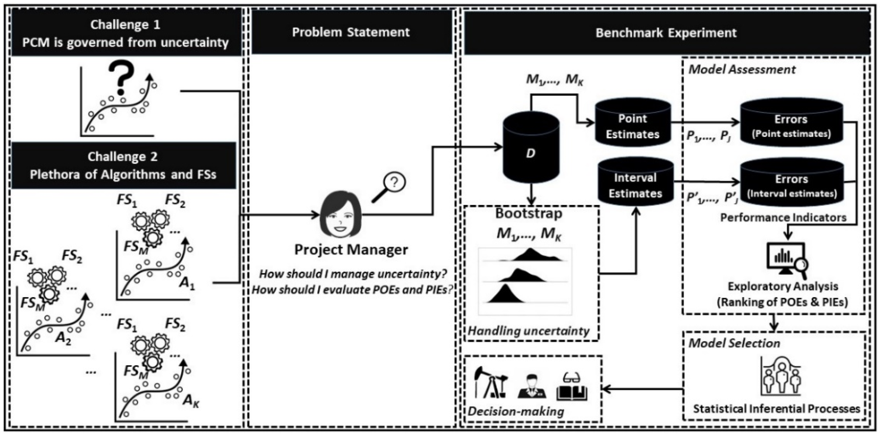
:1. Introduction
2. Background Information
2.1. Prediction System and Probabilistic Uncertainty
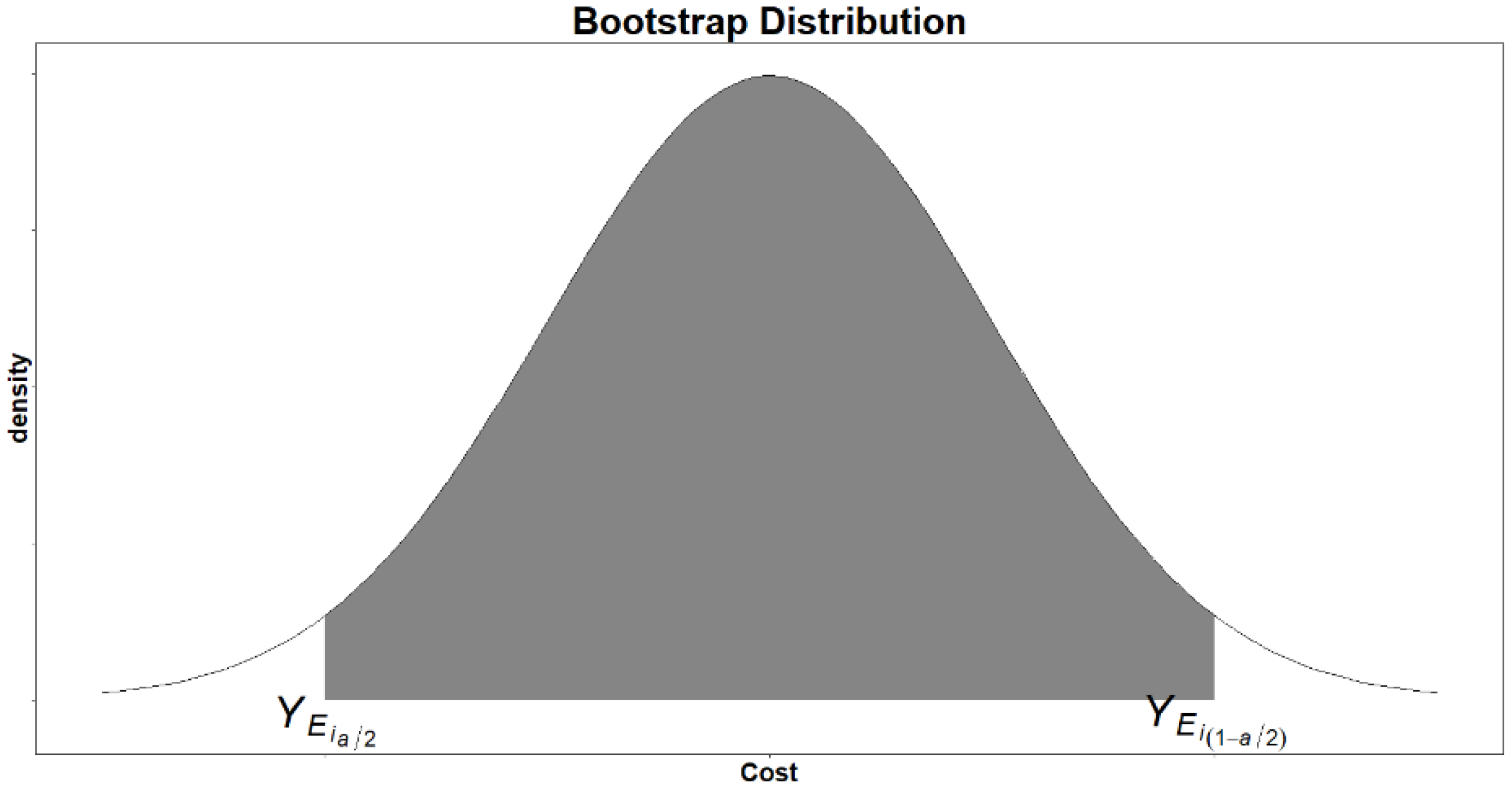
2.2. Non-Parametric Booststrap Resampling
- Obtain a large number of equal-sized samples drawn randomly with replacement from the original random sample .
- For each bootstrap sample , , evaluate an estimate for the unknown parameter of interest .
- The bootstrap estimates form an approximation of the empirical distribution of .
- 1.
- For project
- i.
- Partition the dataset into training and test sets (LOOCV).
- a.
- For each iteration , where denotes a large number of iterations:
- From the set of the projects of the training set , draw randomly with replacement of a set of indices of size .
- Evaluate the cost of the project belonging to the test set, based on the model fitted on the training set.
- b.
- Construct the bootstrap empirical distribution through the estimated values of the project.
- ii.
- Evaluate the PI of the project through the following formula:
- 2.
- Repeat steps (1-i)–(1-ii) for the total number of projects .
2.3. Performance Evaluation and Model Selection
2.3.1. Cost Performance Metrics for Prediction Interval Estimators
2.3.2. Model Selection
3. Research Objectives and Research Questions
4. Experimental Study Design
4.1. Candidate Models
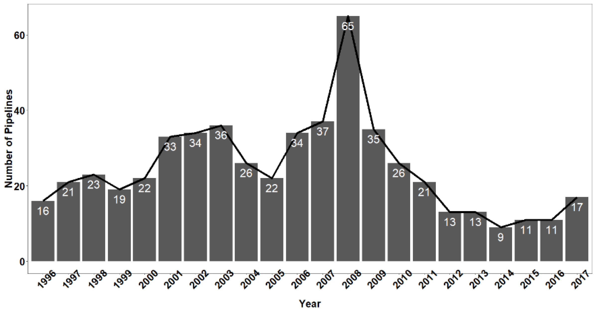
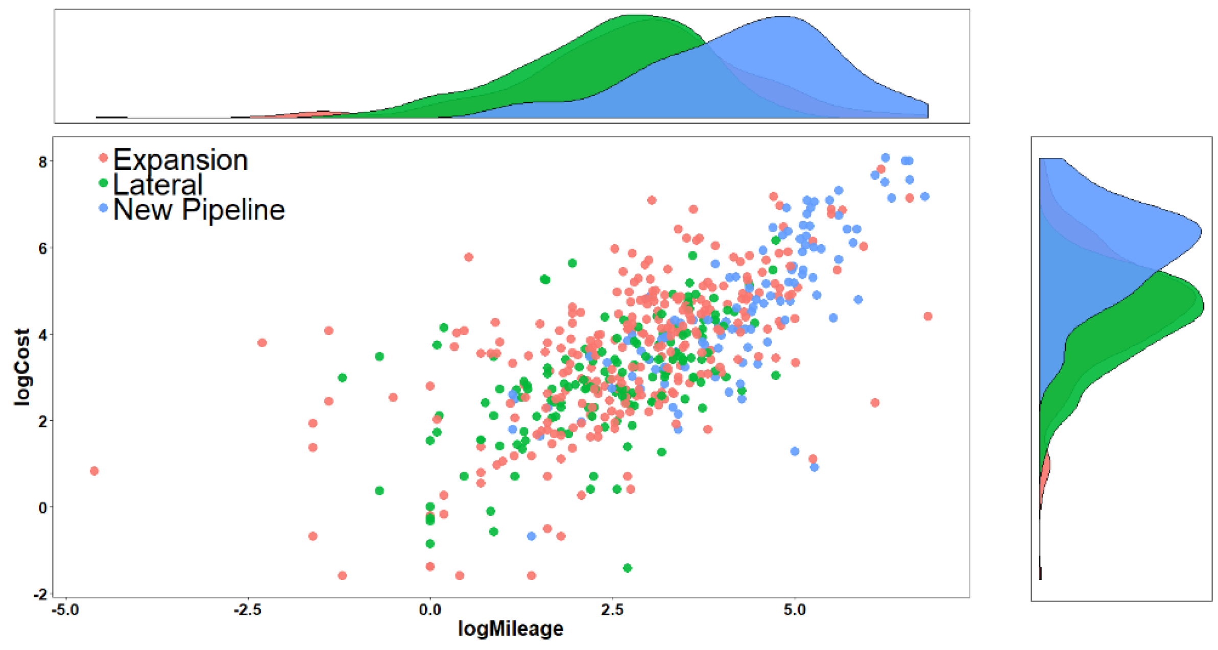
4.2. Dataset
5. Results
5.1. [RQ1] Does the Performance of an Algorithm Providing Point Estimates Depend on the Type of the Applied FSM?
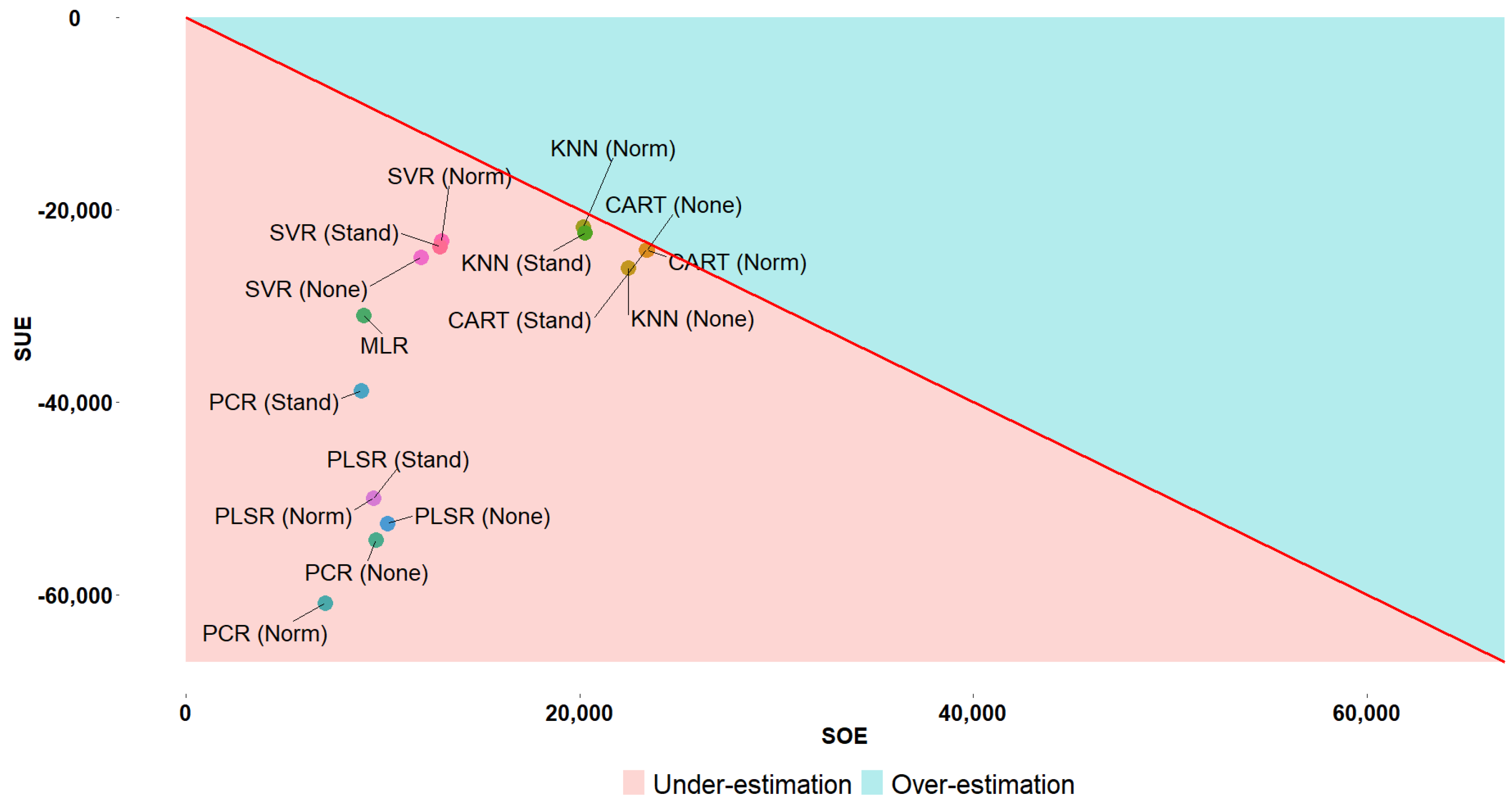
5.2. [RQ2] Is There a Candidate Model (Combination of Algorithm and FSM) Outperforming the Rest in Terms of Point Estimates?
5.3. [RQ3] Does the Performance of an Algorithm Providing Interval Estimates Depend on the Type of the Applied FSM?
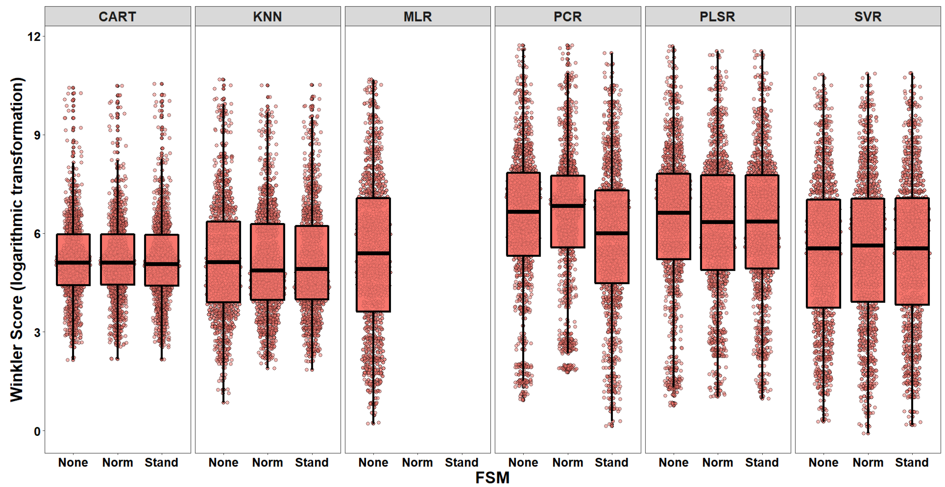
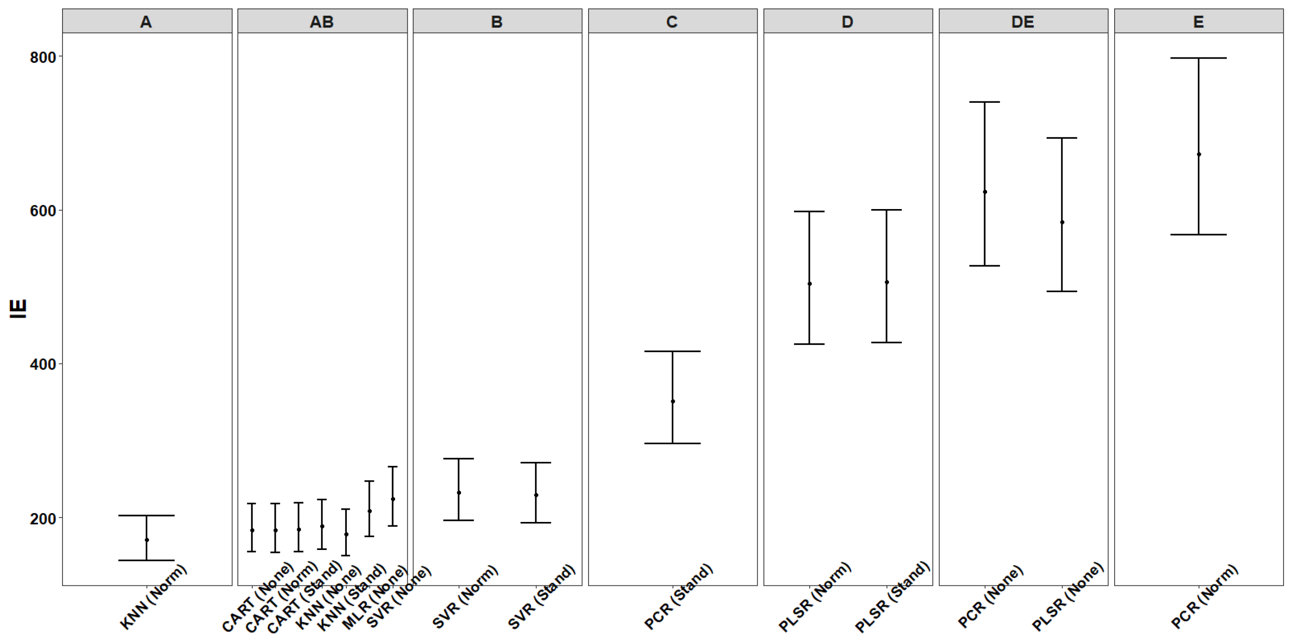
5.4. [RQ4] Is there a Candidate Model (Combination of Algorithm and FSM) Outperforming the Rest in Terms of Interval Estimates? Does the Performance Evaluation in Terms of Point and Interval Estimates Result in a Consistent Ranking of Candidate Models?
6. Threats to Validity
7. Discussion
Author Contributions
Funding
Institutional Review Board Statement
Informed Consent Statement
Data Availability Statement
Conflicts of Interest
References
- Green, J.; Hadden, J.; Hale, T.; Mahdavi, P. Transition, hedge, or resist? Understanding political and economic behavior toward decarbonization in the oil and gas industry. Rev. Int. Polit. Econ. 2021, 1–28. [Google Scholar] [CrossRef]
- Altawell, N. Project management in oil and gas. In Rural Electrification; Altawell, N., Ed.; Academic Press: Cambridge, MA, USA, 2021; pp. 91–107. [Google Scholar]
- Badiru, A.; Osisanya, S. Project Management for the Oil and Gas Industry: A World System Approach; CRC Press: Boca Raton, FL, USA, 2016. [Google Scholar]
- Rui, Z.; Li, C.; Peng, F.; Ling, K.; Chen, G.; Zhou, X.; Chang, H. Development of industry performance metrics for offshore oil and gas project. J. Nat. Gas. Sci. Eng. 2017, 39, 44–53. [Google Scholar] [CrossRef]
- Rui, Z.; Peng, F.; Ling, K.; Chang, H.; Chen, G.; Zhou, X. Investigation into the performance of oil and gas projects. J. Nat. Gas Sci. Eng. 2017, 38, 12–20. [Google Scholar] [CrossRef]
- Rui, Z.; Metz, P.; Reynolds, D.; Chen, G.; Zhou, X. Historical pipeline construction cost analysis. Int. J. Oil Gas Coal Technol. 2011, 4, 244–263. [Google Scholar] [CrossRef]
- Rui, Z.; Metz, P.; Reynolds, D.; Chen, G.; Zhou, X. Regression models estimate pipeline construction costs. Oil Gas J. 2011, 109, 120. [Google Scholar]
- Merrow, E. Oil and gas industry megaprojects: Our recent track record. Oil Gas Facil. 2012, 1, 38–42. [Google Scholar] [CrossRef]
- Rui, Z.; Metz, P.; Chen, G. An analysis of inaccuracy in pipeline construction cost estimation. Int. J. Oil Gas. Coal Technol. 2012, 5, 29–46. [Google Scholar] [CrossRef]
- Rui, Z.; Metz, P.; Chen, G.; Zhou, X.; Wang, X. Regressions allow development of compressor cost estimation models. Oil Gas J. 2012, 110, 110–115. [Google Scholar]
- Rui, Z.; Metz, P.; Wang, X.; Chen, G.; Zhou, X.; Reynolds, D. Inaccuracy in pipeline compressor station construction cost estimation. Oil Gas Facil. 2013, 2, 71–79. [Google Scholar] [CrossRef]
- Rui, Z.; Cui, K.; Wang, X.; Chun, J.H.; Li, Y.; Zhang, Z.; Lu, J.; Chen, G.; Zhou, X.; Patil, S. A comprehensive investigation on performance of oil and gas development in Nigeria: Technical and non-technical analyses. Energy 2018, 158, 666–680. [Google Scholar] [CrossRef]
- Garvin, J. A Guide to Project Management Body of Knowledge; Project Management Institute: Newton Square, PA, USA, 2000. [Google Scholar]
- Stamelos, I.; Angelis, L. Managing uncertainty in project portfolio cost estimation. Inf. Softw. Technol. 2001, 43, 759–768. [Google Scholar] [CrossRef]
- Trendowicz, A.; Jeffery, R. Software Project Effort Estimation. Foundations and Best Practice Guidelines for Success; Springer: Berlin/Heidelberg, Germany, 2014. [Google Scholar]
- Chatfield, C. Calculating interval forecasts. J. Bus. Econ. Stat. 1993, 11, 121–135. [Google Scholar]
- Klassen, R.D.; Flores, B.E. Forecasting practices of Canadian firms: Survey results and comparisons. Int. J. Prod. Econ. 2001, 70, 163–174. [Google Scholar] [CrossRef]
- Goodwin, P.; Önkal, D.; Thomson, M. Do forecasts expressed as prediction intervals improve production planning decisions? Eur. J. Oper. Res. 2010, 205, 195–201. [Google Scholar] [CrossRef]
- Angelis, L.; Stamelos, I. A simulation tool for efficient analogy based cost estimation. Empir. Softw. Eng. 2000, 5, 35–68. [Google Scholar] [CrossRef]
- Christoffersen, P.F. Evaluating interval forecasts. Int. Econ. Rev. 1998, 39, 841–862. [Google Scholar] [CrossRef]
- Solingen, V.R.; Basili, V.; Caldiera, G.; Rombach, H. Goal question metric (GQM) approach. In Encyclopedia of Software Engineering; John and Wiley and Sons: Hoboken, NJ, USA, 2002. [Google Scholar]
- Efron, B.; Tibshirani, R. An Introduction to the Bootstrap; CRC Press: Boca Raton, FL, USA, 1994. [Google Scholar]
- Jochen, V.A.; Spivey, J.P. Probabilistic reserves estimation using decline curve analysis with the bootstrap method. In SPE Annual Technical Conference and Exhibition; OnePetro: Richardson, TX, USA, 1996. [Google Scholar]
- Attanasi, E.D.; Coburn, T.C. A bootstrap approach to computing uncertainty in inferred oil and gas reserve estimates. Nat. Resour. Res. 2004, 13, 45–52. [Google Scholar] [CrossRef]
- Chang, T.; Chen, W.Y.; Gupta, R.; Nguyen, D.K. Are stock prices related to the political uncertainty index in OECD countries? Evidence from the bootstrap panel causality test. Econ. Syst. 2015, 39, 288–300. [Google Scholar] [CrossRef] [Green Version]
- Li, X.L.; Balcilar, M.; Gupta, R.; Chang, T. The causal relationship between economic policy uncertainty and stock returns in China and India: Evidence from a bootstrap rolling window approach. Emerg. Mark. Financ. Trade 2016, 52, 674–689. [Google Scholar] [CrossRef] [Green Version]
- Kondash, A.J.; Albright, E.; Vengosh, A. Quantity of flowback and produced waters from unconventional oil and gas exploration. Sci. Total Environ. 2017, 574, 314–321. [Google Scholar] [CrossRef] [Green Version]
- Kang, W.; De Gracia, F.P.; Ratti, R.A. Oil price shocks, policy uncertainty, and stock returns of oil and gas corporations. J. Int. Money Financ. 2017, 70, 344–359. [Google Scholar] [CrossRef]
- Abumunshar, M.; Aga, M.; Samour, A. Oil price, energy consumption, and CO2 emissions in Turkey. New evidence from a bootstrap ARDL test. Energies 2020, 13, 5588. [Google Scholar] [CrossRef]
- James, G.; Witten, D.; Hastie, T.; Tibshirani, R. An Introduction to Statistical Learning; Springer: Berlin/Heidelberg, Germany, 2013; Volume 112, p. 18. [Google Scholar]
- Hastie, T.; Tibshirani, R.; Friedman, J. The Elements of Statistical Learning: Data Mining Inference and Prediction; Springer: Berlin/Heidelberg, Germany, 2009. [Google Scholar]
- Murphy, K. Machine Learning: A Probabilistic Perspective; MIT Press: Cambridge, MA, USA, 2012. [Google Scholar]
- Kitchenham, B.; Linkman, S. Estimates, uncertainty, and risk. IEEE Softw. 1997, 14, 69–74. [Google Scholar] [CrossRef]
- Kläs, M.; Vollmer, A.M. Uncertainty in machine learning applications: A practice-driven classification of uncertainty. In International Conference on Computer Safety, Reliability, and Security; Springer: Berlin/Heidelberg, Germany, 2018; pp. 431–438. [Google Scholar]
- Ross, S.M. Introduction to Probability and Statistics for Engineers and Scientists; Academic Press: Cambridge, MA, USA, 2020. [Google Scholar]
- Jawad, S.; Ledwith, A. Analyzing enablers and barriers to successfully project control system implementation in petroleum and chemical projects. Int. J. Energy Sect. Manag. 2020, 15, 789–819. [Google Scholar] [CrossRef]
- Hegde, C.M.; Wallace, S.P.; Gray, K.E. Use of regression and bootstrapping in drilling inference and prediction. In SPE Middle East Intelligent Oil and Gas Conference and Exhibition; OnePetro: Richardson, TX, USA, 2015. [Google Scholar]
- Liu, K.; Zhang, Y.; Wang, X. Applications of bootstrap method for drilling site noise analysis and evaluation. J. Pet. Sci. Eng. 2019, 180, 96–104. [Google Scholar] [CrossRef]
- Mittas, N.; Angelis, L. Bootstrap prediction intervals for a semi-parametric software cost estimation model. In Proceedings of the 2009 35th Euromicro Conference on Software Engineering and Advanced Applications, Patras, Greece, 27–29 August 2009; pp. 293–299. [Google Scholar]
- Mittas, N.; Angelis, L. Comparing cost prediction models by resampling techniques. J. Syst. Softw. 2008, 81, 616–632. [Google Scholar] [CrossRef]
- Mittas, N.; Athanasiades, M.; Angelis, L. Improving analogy-based software cost estimation by a resampling method. Inf. Softw. Technol. 2008, 50, 221–230. [Google Scholar] [CrossRef]
- Song, L.; Minku, L.L.; Yao, X. Software effort interval prediction via Bayesian inference and synthetic bootstrap resampling. ACM Trans. Softw. Eng. Methodol. 2019, 28, 1–46. [Google Scholar] [CrossRef]
- Hothorn, T.; Leisch, F.; Zeileis, A.; Hornik, K. The design and analysis of benchmark experiments. J. Comput. Graph. Stat. 2005, 14, 675–699. [Google Scholar] [CrossRef] [Green Version]
- Botchkarev, A. A new typology design of performance metrics to measure errors in machine learning regression algorithms. Interdiscip. J. Inf. Knowl. Manag. 2019, 14, 45. [Google Scholar] [CrossRef] [Green Version]
- Foss, T.; Stensrud, E.; Kitchenham, B.; Myrtveit, I. A simulation study of the model evaluation criterion MMRE. IEEE Trans. Softw. Eng. 2003, 29, 985–995. [Google Scholar] [CrossRef] [Green Version]
- Pal, R. Validation methodologies. In Predictive Modeling of Drug Sensitivity; Academic Press: Cambridge, MA, USA, 2017; pp. 83–107. [Google Scholar]
- Hernández-Orallo, J. ROC curves for regression. Pattern Recognit. 2013, 46, 3395–3411. [Google Scholar] [CrossRef] [Green Version]
- Tripathy, D.; Prusty, R. Forecasting of renewable generation for applications in smart grid power systems. In Advances in Smart Grid Power System; Academic Press: Cambridge, MA, USA, 2021; pp. 265–298. [Google Scholar]
- Casella, G.; Hwang, J. Evaluating confidence sets using loss functions. Stat. Sin. 1991, 1, 159–173. [Google Scholar]
- Troccoli, A.; Harrison, M.; Anderson, D.L.; Mason, S.J. Seasonal Climate: Forecasting and Managing Risk; Springer: Berlin/Heidelberg, Germany, 2008; Volume 82. [Google Scholar]
- Gneiting, T.; Raftery, A. Strictly proper scoring rules, prediction, and estimation. J. Am. Stat. Assoc. 2007, 102, 359–378. [Google Scholar] [CrossRef]
- Wang, H. Closed form prediction intervals applied for disease counts. Am. Stat. 2010, 64, 250–256. [Google Scholar] [CrossRef] [Green Version]
- Khosravi, A.; Nahavandi, S.; Creighton, D. Construction of optimal prediction intervals for load forecasting problems. IEEE Trans. Power Syst. 2010, 25, 1496–1503. [Google Scholar] [CrossRef] [Green Version]
- Landon, J.; Singpurwalla, N.D. Choosing a coverage probability for prediction intervals. Am. Stat. 2008, 62, 120–124. [Google Scholar] [CrossRef]
- Winkler, R.L. A decision-theoretic approach to interval estimation. J. Am. Stat. Assoc. 1972, 67, 187–191. [Google Scholar] [CrossRef]
- Dietterich, T. Approximate statistical tests for comparing supervised classification learning algorithms. Neural Comp. 1998, 10, 1895–1923. [Google Scholar] [CrossRef] [Green Version]
- Demšar, J. Statistical comparisons of classifiers over multiple data sets. J. Mach. Learn. Res. 2006, 7, 1–30. [Google Scholar]
- Garcia, S.; Herrera, F. An extension on “statistical comparisons of classifiers over multiple data sets” for all pairwise comparisons. J. Mach. Learn. Res. 2008, 9, 2677–2694. [Google Scholar]
- Mittas, N.; Angelis, L. Ranking and clustering software cost estimation models through a multiple comparisons algorithm. IEEE Trans. Softw. Eng. 2013, 39, 537–551. [Google Scholar] [CrossRef]
- Jiang, J. Linear and Generalized Linear Mixed Models and Their Applications; Springer: Berlin/Heidelberg, Germany, 2007. [Google Scholar]
- Pinheiro, J.; Bates, D. Mixed-Effects Models in S and S-PLUS; Springer: Berlin/Heidelberg, Germany, 2006. [Google Scholar]
- Millar, R.B.; Anderson, M.J. Remedies for pseudoreplication. Fish. Res. 2004, 70, 397–407. [Google Scholar] [CrossRef]
- Guyon, I.; Gunn, S.; Nikravesh, M.; Zadeh, L. Feature Extraction: Foundations and Applications; Springer: Berlin/Heidelberg, Germany, 2008; Volume 207. [Google Scholar]
- Zuur, A.; Ieno, E.; Walker, N.; Saveliev, A.; Smith, G. Mixed Effects Models and Extensions in Ecology with R; Springer: Berlin/Heidelberg, Germany, 2009. [Google Scholar]
- Breiman, L.; Friedman, J.; Stone, C.; Olshen, R.A. Classification and Regression Trees; Taylor & Francis: Abingdon, UK, 1984. [Google Scholar]
- Härdle, W. Applied Non-Parametric Regression; Cambridge University Press: Cambridge, UK, 1990. [Google Scholar]
- Jolliffe, I. Principal Component Analysis; Springer: Berlin/Heidelberg, Germany, 2011. [Google Scholar]
- Vapnik, V.; Golowich, S.; Smola, A. Support vector method for function approximation, regression estimation and signal processing. In Advances in Neural Information Processing Systems; MIT Press: Cambridge, MA, USA, 1997; pp. 281–287. [Google Scholar]
- Kuhn, M. Building predictive models in R using the caret package. J. Stat. Softw. 2008, 28, 1–26. [Google Scholar] [CrossRef] [Green Version]
- R Core Team. R: A Language and Environment for Statistical Computing; R Foundation for Statistical Computing: Vienna, Austria, 2014. [Google Scholar]
- International Energy Agency. World Energy Investment, Executive Summary; International Energy Agency: Paris, France, 2018. [Google Scholar]
- García, S.; Fernández, A.; Luengo, J.; Herrera, F. Advanced nonparametric tests for multiple comparisons in the design of experiments in computational intelligence and data mining: Experimental analysis of power. Inf. Sci. 2010, 180, 2044–2064. [Google Scholar] [CrossRef]
- Hornik, K.; Meyer, D. Deriving consensus rankings from benchmarking experiments. In Advances in Data Analysis; Springer: Berlin/Heidelberg, Germany, 2007; pp. 163–170. [Google Scholar]
- Lenth, R. Using lsmeans. J. Stat. Softw. 2017, 9, 1–33. [Google Scholar]
- Sheskin, D. Handbook of Parametric and Nonparametric Statistical Procedures; CRC Press: Boca Raton, FL, USA, 2003. [Google Scholar]
- Krippendorff, K. Estimating the reliability, systematic error and random error of interval data. Educ. Psychol. Meas. 1970, 30, 61–70. [Google Scholar] [CrossRef]
- Calder, B.; Phillips, L.; Tybout, A. The concept of external validity. J. Consum. Res. 1982, 9, 240–244. [Google Scholar] [CrossRef]


| Approach | Component | Scope |
|---|---|---|
| Non-parametric bootstrap [19,22,39,42] | Handling of uncertainty | Production of interval estimates of cost |
| Loss functions for point estimators [44] | Model Assessment | Performance evaluation of point estimators |
| Regression Receiver Operating Curves (RROC) space [47] | Model Assessment | Graphical investigation of the tendency of point estimators to under- or over-estimate the actual cost |
| Loss functions for interval estimators [20,48,55] | Model Assessment | Performance evaluation of interval estimators |
| Linear Mixed Effects models [61] | Model Selection | Modeling the fixed and random effects on the distributions evaluated by continuous loss functions (AE, Width, Winkler Score) |
| Generalized Linear Mixed Models (with logit link function) [61] | Model Selection | Modeling the fixed and random effects on the distributions of the indicator variable expressing whether the actual cost lies within the produced interval |
| Model (Combination of Algorithm and FSM) | Tuning Parameters | Best Value | R Function (Package) |
|---|---|---|---|
| MLR (None) | No tuning parameters | - | lm (stats) |
| CART (None) | complexity parameter cp = {0.0001, 0.001, 0.01, 0.1, 0.5} | 0.0001 | rpart (rpart) |
| CART (Norm) | 0.0001 | ||
| CART (Stand) | 0.0001 | ||
| KNN (None) | number of nearest neighbors nn = {1:20} | 4 | knnreg (caret) |
| KNN (Norm) | 3 | ||
| KNN (Stand) | 4 | ||
| PCR (None) | number of components nc = {1:(#predictors-1)} | 3 | pcr (pls) |
| PCR (Norm) | 3 | ||
| PCR (Stand) | 3 | ||
| PLSR (None) | 5 | plsr (pls) | |
| PLSR (Norm) | 5 | ||
| PLSR (Stand) | 5 | ||
| SVR (None) | Cost of constraint violation C = {21, 22, 23, 24, 25, 26} epsilon insensitive-loss epsilon = {0.1:1, by 0.01} | C = 4, epsilon = 0.30 | ksvm (kernlab) |
| SVR (Norm) | C = 4, epsilon = 0.15 | ||
| SVR (Stand) | C = 4, epsilon = 0.25 |
| Name | Definition | Type | Levels |
|---|---|---|---|
| Cost ($M) | Projects estimated cost based on companies’ press releases or applications | Continuous | |
| Mileage (Miles) | Projects estimated mileage based on companies’ press releases or applications | Continuous | |
| Capacity (MMcf/d) | Projects estimated additional capacity based on companies’ press releases or applications | Continuous | |
| Diameter (Inches) | Pipeline estimated diameter based on companies’ press releases or applications | Continuous | |
| Project Type | Type of project | Categorical | Expansion, Lateral, New Pipeline |
| Pipeline Type | Type of pipeline | Categorical | Interstate, Intrastate |
| Year | The date when the projects were completed or put in service | Discrete |
| Variable (Continuous) | M | SD | Mdn | min | max |
|---|---|---|---|---|---|
| Cost ($M) | 144.28 | 352.86 | 36.00 | 0.20 | 3200 |
| Mileage (Miles) | 55.88 | 107.52 | 20.95 | 0.01 | 922 |
| Capacity (MMcf/d) | 330.30 | 426.36 | 180.00 | 1.70 | 2600 |
| Diameter (Inches) | 25.69 | 10.06 | 24.00 | 4.00 | 48 |
| Variable (Categorical) | Level | N | % | ||
| Project Type | Expansion | 276 | 50.7 | ||
| Lateral | 158 | 29.0 | |||
| New Pipeline | 110 | 20.2 | |||
| Pipeline Type | Interstate | 446 | 82.0 | ||
| Intrastate | 98 | 18.0 | |||
| Model | Performance Metrics | |||||||
|---|---|---|---|---|---|---|---|---|
| Point Estimators | Prediction Interval Estimators | |||||||
| Algorithm | FSM | MAE | MdAE | CP (%) | MWidth | MdWidth | MWS | MdWS |
| CART | None | 87.51 | 21.37 | 73.35 | 253.88 | 118.96 | 759.63 | 164.51 |
| Norm | 87.51 | 21.37 | 74.63 | 255.65 | 118.86 | 748.84 | 165.41 | |
| Stand | 87.45 | 21.18 | 74.26 | 254.27 | 117.60 | 772.73 | 158.23 | |
| KNN | None | 89.23 | 22.20 | 63.42 | 202.48 | 75.23 | 1236.84 | 166.67 |
| Norm | 77.15 | 21.59 | 66.91 | 197.59 | 72.56 | 918.80 | 130.51 | |
| Stand | 78.50 | 23.85 | 63.24 | 183.83 | 72.47 | 996.03 | 136.27 | |
| MLR | None | 73.54 | 13.20 | 27.39 | 55.16 | 14.27 | 2034.15 | 218.61 |
| PCR | None | 117.67 | 27.35 | 11.03 | 25.33 | 7.23 | 4254.13 | 766.89 |
| Norm | 124.93 | 30.59 | 14.71 | 23.06 | 14.39 | 4583.58 | 919.33 | |
| Stand | 87.73 | 18.18 | 17.83 | 39.11 | 9.96 | 2822.88 | 402.76 | |
| PLSR | None | 115.51 | 25.16 | 12.13 | 26.04 | 7.10 | 4149.49 | 750.25 |
| Norm | 109.47 | 23.71 | 15.26 | 40.23 | 13.75 | 3645.41 | 565.40 | |
| Stand | 109.47 | 23.71 | 15.26 | 40.21 | 13.88 | 3643.54 | 568.97 | |
| SVR | None | 67.84 | 14.04 | 23.90 | 48.07 | 13.94 | 1911.85 | 252.26 |
| Norm | 66.67 | 13.06 | 22.98 | 45.75 | 12.96 | 1901.21 | 278.06 | |
| Stand | 67.56 | 14.66 | 24.45 | 45.80 | 13.40 | 1921.40 | 252.16 | |
| Performance Metric | MEM | Fixed Component Structure | df | AIC | Comparison |
|---|---|---|---|---|---|
| AE | LMEM A | 18 | 27219 | Model A vs. Model B | |
| LMEM B | 10 | 27284 | |||
| Indicator variable of Coverage | GLMM A | 17 | 7799.0 | Model A vs. Model B | |
| GLMM B | 9 | 7799.2 | |||
| GLMM C | Algorithm | 7 | 7796.1 | Model B vs. Model C | |
| Width | LMEM A | 18 | 18248 | Model A vs. Model B | |
| LMEM B | 10 | 18429 | |||
| WS | LMEM A | 18 | 30928 | Model A vs. Model B | |
| LMEM B | 10 | 30980 |
| AE | Indicator Variable of Coverage | Width | WS | |||||||
|---|---|---|---|---|---|---|---|---|---|---|
| Algorithm | FSM | Group | Algorithm | Group | Algorithm | FSM | Group | Algorithm | FSM | Group |
| MLR | None | A | CART | A | PLSR | None | A | KNN | Norm | A |
| SVR | Norm | A | KNN | B | PCR | None | A | KNN | Stand | AB |
| SVR | None | AB | MLR | C | PCR | Stand | AB | CART | None | AB |
| SVR | Stand | AB | SVR | C | SVR | Norm | BC | CART | Norm | AB |
| PCR | Stand | B | PCR | D | SVR | Stand | CD | CART | Stand | AB |
| CART | Stand | C | PLSR | D | SVR | None | CDE | KNN | None | AB |
| CART | None | C | MLR | None | DE | MRL | None | AB | ||
| CART | Norm | C | PCR | Norm | DE | SVR | None | AB | ||
| KNN | Norm | C | PLSR | Stand | E | SVR | Stand | B | ||
| KNN | None | C | PLSR | Norm | E | SVR | Norm | B | ||
| KNN | Stand | C | KNN | Stand | F | PCR | Stand | C | ||
| PLSR | None | C | KNN | None | F | PLSR | Norm | D | ||
| PCR | None | C | KNN | Norm | F | PLSR | Stand | D | ||
| PLSR | Norm | CD | CART | Stand | G | PLSR | None | DE | ||
| PLSR | Stand | CD | CART | None | G | PCR | None | DE | ||
| PCR | Norm | D | CART | Norm | G | PCR | Norm | E | ||
Publisher’s Note: MDPI stays neutral with regard to jurisdictional claims in published maps and institutional affiliations. |
© 2022 by the authors. Licensee MDPI, Basel, Switzerland. This article is an open access article distributed under the terms and conditions of the Creative Commons Attribution (CC BY) license (https://creativecommons.org/licenses/by/4.0/).
Share and Cite
Mittas, N.; Mitropoulos, A. A Data-Driven Framework for Probabilistic Estimates in Oil and Gas Project Cost Management: A Benchmark Experiment on Natural Gas Pipeline Projects. Computation 2022, 10, 75. https://0-doi-org.brum.beds.ac.uk/10.3390/computation10050075
Mittas N, Mitropoulos A. A Data-Driven Framework for Probabilistic Estimates in Oil and Gas Project Cost Management: A Benchmark Experiment on Natural Gas Pipeline Projects. Computation. 2022; 10(5):75. https://0-doi-org.brum.beds.ac.uk/10.3390/computation10050075
Chicago/Turabian StyleMittas, Nikolaos, and Athanasios Mitropoulos. 2022. "A Data-Driven Framework for Probabilistic Estimates in Oil and Gas Project Cost Management: A Benchmark Experiment on Natural Gas Pipeline Projects" Computation 10, no. 5: 75. https://0-doi-org.brum.beds.ac.uk/10.3390/computation10050075