
A Mathematical and Numerical Framework for Traffic-Induced Air Pollution Simulation in Bamako


Département d’Enseignement et de Recherche en Mathématique et Informatique, Faculté des Sciences et Techniques, Université des Sciences, des Techniques et des Technologies de Bamako, Bamako BPE 423, Mali
*
Author to whom correspondence should be addressed.
Computation 2022, 10(5), 76; https://0-doi-org.brum.beds.ac.uk/10.3390/computation10050076
Submission received: 18 March 2022
/
Revised: 15 April 2022
/
Accepted: 6 May 2022
/
Published: 17 May 2022
Abstract
:We present a mathematical and numerical framework for the simulation of traffic-induced air pollution in Bamako. We consider a deterministic modeling approach where the spatio-temporal dynamics of the concentrations of air pollutants are governed by a so-called chemical transport model. The time integration and spatial discretization of the model are achieved using the forward Euler algorithm and the finite-element method, respectively. The traffic emissions are estimated using a road traffic simulation package called SUMO. The numerical results for two road traffic-induced air pollutants, namely the carbon monoxide (CO) and the fine particulate matter (PM), support that the proposed framework is suited for reproducing the dynamics of the pollutants specified.
1. Introduction
Air pollution is nowadays a major risk factor for human health and a global environmental concern. It is even more worrying in urban areas because of a high concentration of population and a sustained increase in the road transport fleet [1]. There are two principal types of air pollutants: primary pollutants and secondary pollutants. The primary pollutants are directly emitted into the atmosphere from natural sources, including wildfires and volcanic eruptions, or anthropogenic sources, including industries and road traffic. As for secondary pollutants, they are formed within the atmosphere as the result of chemical reactions of primary pollutants. The most common acute and chronic illnesses associated with air pollution include lung cancer, nose and throat (ENT) disorders, chronic obstructive pulmonary disease (COPD), and cardiovascular diseases. The World Health Organization (WHO) reports that the ambient air pollution is responsible for 4.2 million premature deaths worldwide every year [2]. The outdoor air pollution has been classified as carcinogenic to humans [3] by the International Agency for Research on Cancer (IARC), the specialized cancer agency of the WHO. Faced with this serious public health and environmental issues, policies have been implemented at local and international scales for regulating and monitoring air pollution. A strategy commonly adopted, mainly in advanced countries, consists of monitoring the concentrations of the pollutants of interest on a network of fixed monitoring stations using air quality sensors. This approach is not always viable since these monitors are often expensive, especially for developing countries.
Thanks to the fast acceleration in computational power and continuous progress in robust numerical algorithms, the modeling and simulation of air pollution are alternatives that work well [4]. Air pollution modeling is a complex scientific problem that involves the transport and dispersion of the air pollutants [5] as well as the processes related to the deposition and chemical reactions.
In the literature [6], there are two main types of mathematical methods that express air pollution processes: statistical models and deterministic models. The statistical models are based on the semi-empirical statistical relationships between various data and available measurement. As for deterministic models, they focused on the mathematical description of the physical and chemical processes in the atmosphere. The deterministic models are most suitable for practical applications and are, in general, more accurate and flexible. There are currently two fundamental methods [7] that address the turbulent diffusion: the Eulerian scheme and the Lagrangian approach. The main idea in the Eulerian models is to numerically solve the atmospheric transport equation in a fixed coordinate frame, while the Lagrangian models calculate the trajectories of air pollutants driven by deterministic and stochastic effects.
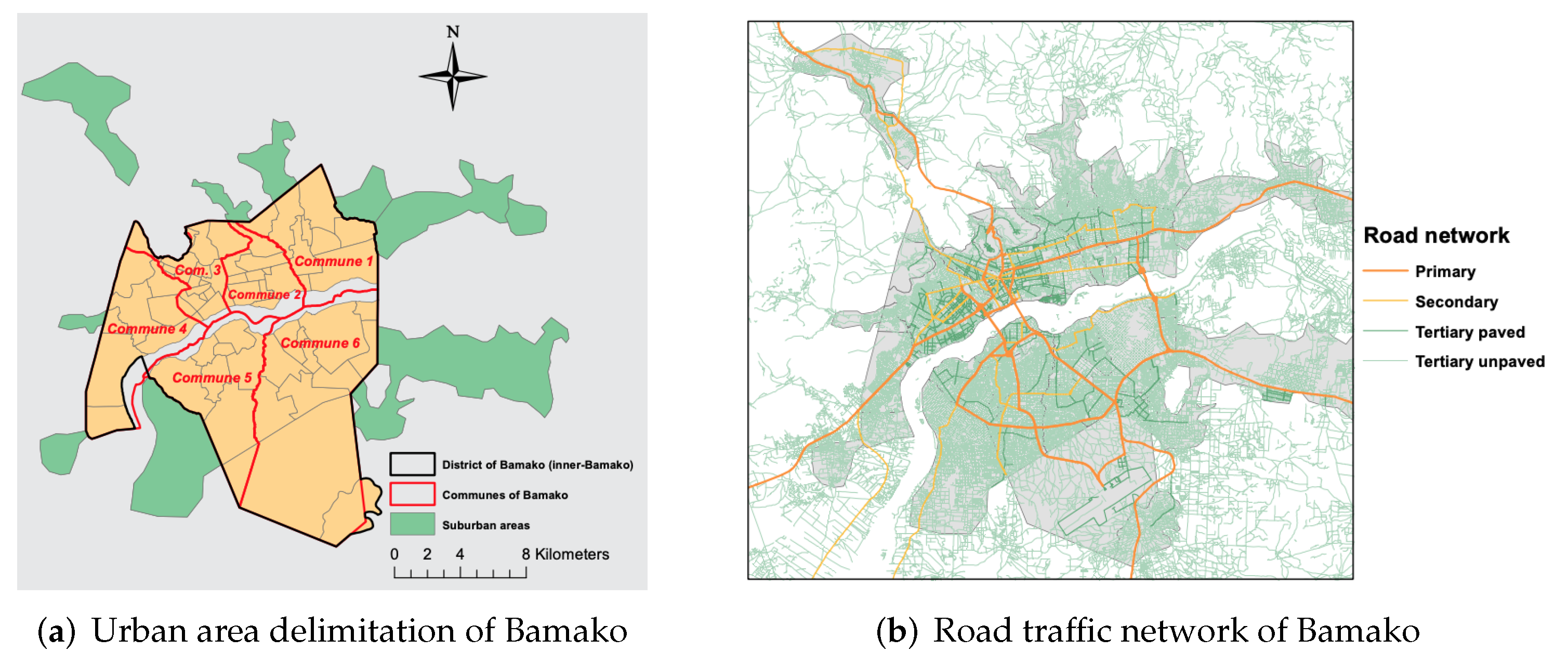
The City of Bamako, which is the political and economic capital of Mali, is located at latitude 12°38′21″ N and longitude 8°0′10″ W and straddles the Niger River in the southwestern part of Mali, see Figure 1. It represents only about 0.02% of the total area of the country but is home to nearly 12.46% of the Malian population. The population density in this city is estimated to 9062 people per km [8]. Bamako represents the most important commercial crossroads of Mali since it concentrates about 70% of the economic activities of the country. These robust economic activities, coupled with a fast population increase, are factors that amplify the effects of pollution in Bamako. Despite recent advances in engine technology, the traffic flow continues to be the principal source of air pollution in urban areas [9], especially in Bamako, where the obsolescence of the transport infrastructure, see Figure 2, and the aging of the transport fleet make the pollution worse.
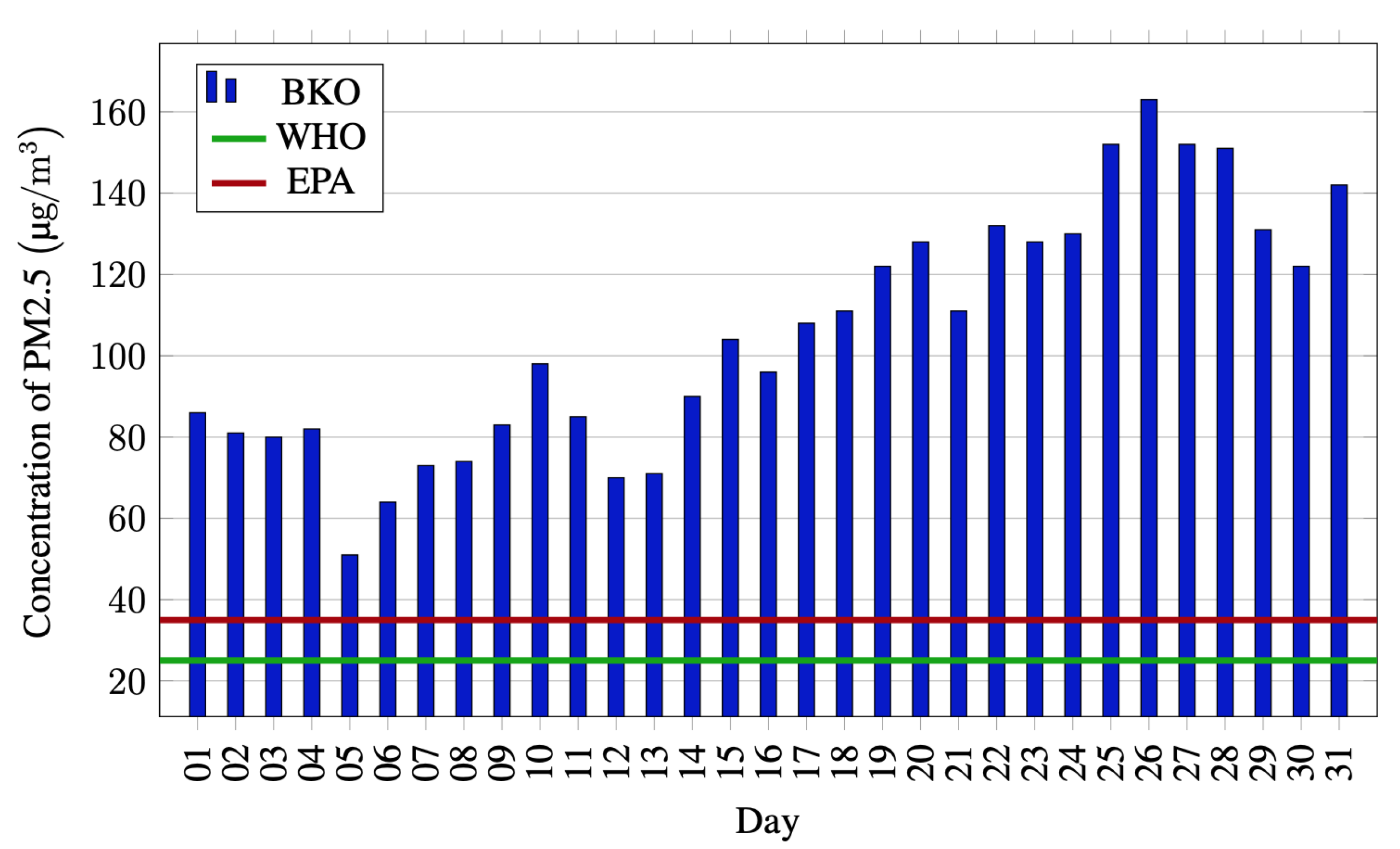
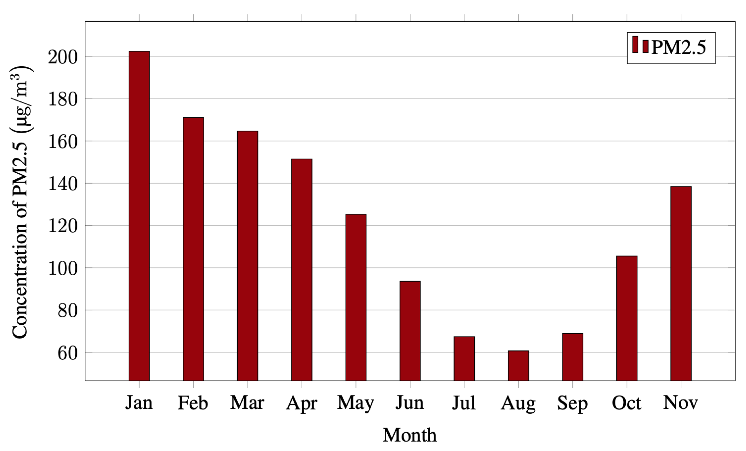
We focus on two primary pollutants widely used in the study and in the forecast of air pollution, namely the inhalable particulate matter less than 10 in aerodynamic diameter called PM and the fine particulate matter less than in aerodynamic diameter called PM. In Bamako, the daily averaged PM concentration can reach a peak of 600 /m3 [10] while the daily maximum limit recommended by the WHO guideline is 45 /m3. On the other hand, the daily and monthly mean PM concentrations over the month of October 2020 are reported in the Figure 3 and Figure 4, respectively. As shown in Figure 3, the daily PM concentrations reach a peak of 165 /m3 while the daily maximum limit recommended by the WHO is fixed 15 /m3 [11].
These factors mentioned above support that the air pollution level in Bamako is very worrying. It is therefore essential to implement control and monitoring mechanisms for reducing the health and environmental impacts of the air pollution. For this purpose, we introduced in this paper a non-trivial application of the modeling and simulation of air pollution in Bamako in order to contribute to a better understanding of the dispersion pattern of road traffic-related air pollutants and to help in the decision-making process for a better regulation of the traffic emissions. It will thus make it possible to more precisely assess a possible correlation between the level of air pollution in Bamako and the frequency of diagnosis of certain diseases whose causes are still not identified. In terms of specific contribution to the current literature, this paper provides the scientific community interested in air pollution issues with a practical application based on new robust advanced numerical tools. To this end, it could serve as kernel for the implementation of eventual pollution models in other large African cities highly impacted by the effects of air pollution.
As the statistical models are in general not accurate enough for long term air pollution simulations, we consider in this framework a deterministic and Eulerian-based modeling approach. Although mathematical modeling and simulation are key tools for urban air pollution assessment, they are often challenging to implement and require high computational costs. In this work, the numerical simulations were performed using a scalable parallel computational framework proposed in [12]. The traffic emissions data required for running air pollution simulations were estimated using a useful road traffic simulation package called SUMO.
The paper is organized as follows. Section 2 describes the mathematical model and the initial and boundary conditions. In Section 3, we present the computational mesh generation processes. Section 4 details the traffic simulation modeling and emissions. In Section 5, we present the numerical results and discuss their interpretations. Section 6 focuses on the validation of the numerical results using observational data. The main conclusions are recapped in Section 7.
2. Model Description
Let be a bounded domain of , see Figure 5. Let the boundary of . We denote by c the vector field of concentrations, where the component represents the scalar concentration field of the air pollutant labeled i. The spatial and temporal dynamics of the concentration in the computational domain over the time interval are governed by the following atmospheric chemical transport model:
where
- (i)
- : concentration of pollutant labeled i;
- (ii)
- : diffusion coefficient;
- (iii)
- : wind flow speed;
- (iv)
- : sources of chemical reactions;
- (v)
- : scavenging coefficient;
- (vi)
- : source terms;
- (vii)
- : spatial variables, where z represents the altitude;
- (viii)
- t: model time.
Table 1 summarizes the parameters and physical fields presented above and their units.
In model (1), we neglect the feedback between the pollutants and the flow fields. The flow is supposed to be incompressible and the urban terrain is assumed to be homogeneous. The wind velocity is traditionally provided by meteorological models [15]. We focus on a maximum altitude H included in the atmospheric boundary layer [16].
2.1. Initial and Boundary Conditions
Equation (1) is supplemented by initial and boundary conditions. We suppose that the region of interest, i.e., the computational domain, is free of pollution at the beginning of the emission, i.e., . The boundary of shown in Figure 5a is decomposed as:
where denotes the ground boundary of and is the upper limit of . The subsets , , and are lateral boundaries. The boundary conditions on the ground surface are given by a contribution of deposits and emissions. They are the following form:
where is the surface emissions of the species labeled i emitted from road traffic, denotes the unit outward vector normal to the boundary . The field refers to the dry deposition velocity [6], see Section 2.2 for more details. On the upper limit boundary , the boundary conditions are given by a zero diffusive pollution flow:
On the lateral boundaries, no pollution sources outside the domain are considered, i.e., the advective pollution flow is assumed to be zero:
2.2. Dry Deposition and Scavenging Processes
The dry deposition refers to the direct transfer of species to the ground without the aid of precipitation [17]. It constitutes a loss term and its intensity depends on the pollutants, meteorological conditions and season. The dry deposition flux [18] related to the species labeled i is computed as follows:
The dry deposition velocity is parameterized by chemical species. It is a function of the meteorological conditions in the surface boundary layer and the type of soil characterized by the land use coverage (LUC) and the specific roughness parameter ([15], [Table 3.5]). Some typical values of as a function of LUC are reported in ([19], [Table 3]). An illustration of the evolution of as a function of the size of particles for some specific values of the wind velocity is presented in ([15], [Figure 3.24]).
The loss due to the mass transfers with the aqueous phase (clouds or rain) is called wet deposition or wet scavenging. The soluble pollutants can penetrate raindrops when they fall; thus, they are precipitated on the ground. This type of deposit is known as below-cloud scavenging (BCS). Another form of wet scavenging takes place in the clouds where the soluble pollutants interacts (mass transfers) with the drops of water. This type of deposit is known as in-cloud scavenging (ICS). The wet scavenging plays a major role for gas-phase soluble species and aerosols since it governs their residence time in the atmosphere. Although the rainfall are a key process in pollution models, they generally focus on BCS wet scavenging since there is insufficient data on ICS wet deposition [20]. The scavenged concentrations satisfy the following time evolution:
The coefficient , called scavenging coefficient, is the parametrization of all processes that result in scavenging. It is a function depending on the rain properties and the scavenged matter. Through numerous observational data, it follows that the scavenging coefficient for the aerosols can be configured as follows ([15], [Chapter 5, Section 5.3.2]):
where (in mm h) is the rainfall intensity. The coefficients and are specific constants that depend on aerosols. For the coarse fraction of aerosols distribution (diameters greater than 1 m), typical values of and are: and . For the submicronic fraction of aerosols distribution (diameters less than 1 m), we have: and .
Some tables presented in [19] report typical values of and , sometimes obtained from experimental data, as a function of the size of the aerosols. An illustration of the scavenging coefficient as a function of the size of the aerosols for different intensities of the rain is presented in ([19], [Figure 3]).
2.3. Chemical Kinetics
The temporal evolution of the concentrations of pollutants due to the chemical kinetics in the reactive dispersion Equation (1) is described by the following system of ordinary differential equations:
where n is the number of species. This time integration of chemical kinetics is very challenging [21]. The first difficulty is related to the size of of the system (9), which can be very large (). The second issue is associated with the non-linearity of the system (9) since the species are coupled together through chemical reactions. Many explicit or quasi-explicit methods devoted to the solution of this system are available in the literature [21]. Among them, the class of methods known as QSSA (quasi steady state assumption) [22] is still widely used. It is based on the so-called production-consumption form of the chemical reaction:
where and represents the production and loss term, respectively. If we consider the first-order chemical reaction, then and are constants and the concentration is expressed in the form:
with a characteristic timescale of . By extension, the characteristic timescale of the pollutant labeled i is computed as:
The characteristic timescale for the species labeled i is computed from the dry deposition velocity and the maximum altitude H as follows:
3. Computational Mesh Processing
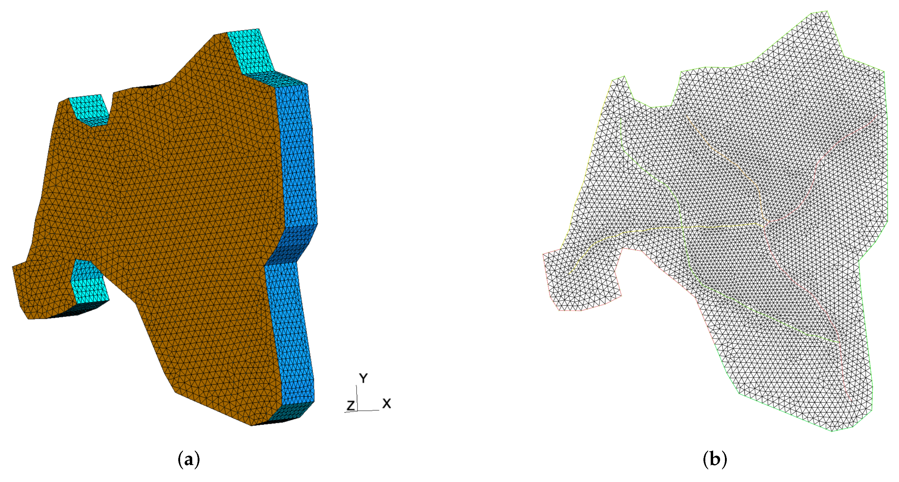
We start this step by extracting a map of Bamako from the OpenStreetMap (OSM) [23], a collaborative project for a free editable map of the world. This map contains, among others, the information on buildings, road networks and geospatial data initially expressed in the World Geodetic System 1984 (WGS 84). It has been processed and edited using an extensible editor for OSM data called JOSM [24]. For reasons of simplification, we have only considered the road networks and other useful information associated with them. Then, the map was imported into an open-source geographic information system called QGIS [25], from which, a geometry input file for the mesh generator Gmsh [26] was created using an external plugin. We exported the built geometry file according to the Universal Transverse Mercator (UTM) Coordinate System, zone 29N. Finally, a three-dimensional (3D) computational mesh over the region of interest was generated from the geometry file using Gmsh. This three-dimensional computational mesh and the ground boundary mesh extracted from it are plotted in Figure 6a,b, respectively.
4. Traffic Simulation Model
The emissions data are required for initializing a simulation of air pollution. Since experiments with traffic networks in real-life environment are often difficult, even impractical, the traffic flow simulation models [27] are common tools used to analyze traffic operations, assess traffic management strategies and report emission rates of pollutants. The traffic-induced emissions studied in this framework were estimated using SUMO [28]—Simulation of Urban MObility. SUMO is an open-source, microscopic and continuous multi-modal road traffic simulation package dedicated to handle large and complex road networks [29]. We carried out traffic simulations on the main and most frequented roads of the city of Bamako, see Figure 5b. These roads are susceptible to severe traffic congestion over peak hours, mainly from 7 a.m. to 11 a.m. on working days. The main data required for traffic simulations using SUMO were obtained from the Malian department of transport and infrastructure.
5. Numerical Experiments
In this framework, we are interested in two traffic-induced primary pollutants, namely carbon monoxide (CO) and fine particulate matter (PM). The CO is an odorless, colorless and tasteless gas emitted in the city mainly by motor vehicles, far ahead of the concentration emitted during combustion processes. The choice of this pollutant is motivated by the fact that its exposure remains one of the leading causes of unintentional poisonings worldwide [30]. Regarding the widespread air pollutant PM, its choice is inspired by the fact that the short-term exposures to these loads have been associated with several respiratory diseases.
We consider a first-order chemical reaction, see Section 2.3; therefore the balance of the physico-chemical transformations is written in the form , where denotes the rate of the reaction. The losses due to the deposit and scavenging are assumed to be negligible, which results in . The physico-chemical parameters corresponding to CO are m s and s . The physico-chemical parameters for PM are given by: m s and s . We consider a maximum altitude m. The dry deposition velocity is computed as . The time step is set to 60 . The three-dimensional mesh used for the simulations and the two-dimensional mesh of the ground boundary are presented in Figure 6. The wind data used for the simulations have a resolution of 10 and were obtained from the European Centre for Medium-Range Weather Forecasts (ECMWF). The first-order finite-element approximation is used for the spatial discretization of the model.
The simulations were carried out on the “Centre de Calcul, Modélisation et Simulation” (CCMS) of the Faculty of Sciences and Technologies (FST) of Bamako using the parallel and scalable computational framework presented in [12]. The configurations of the cluster CCMS are also described in [12].
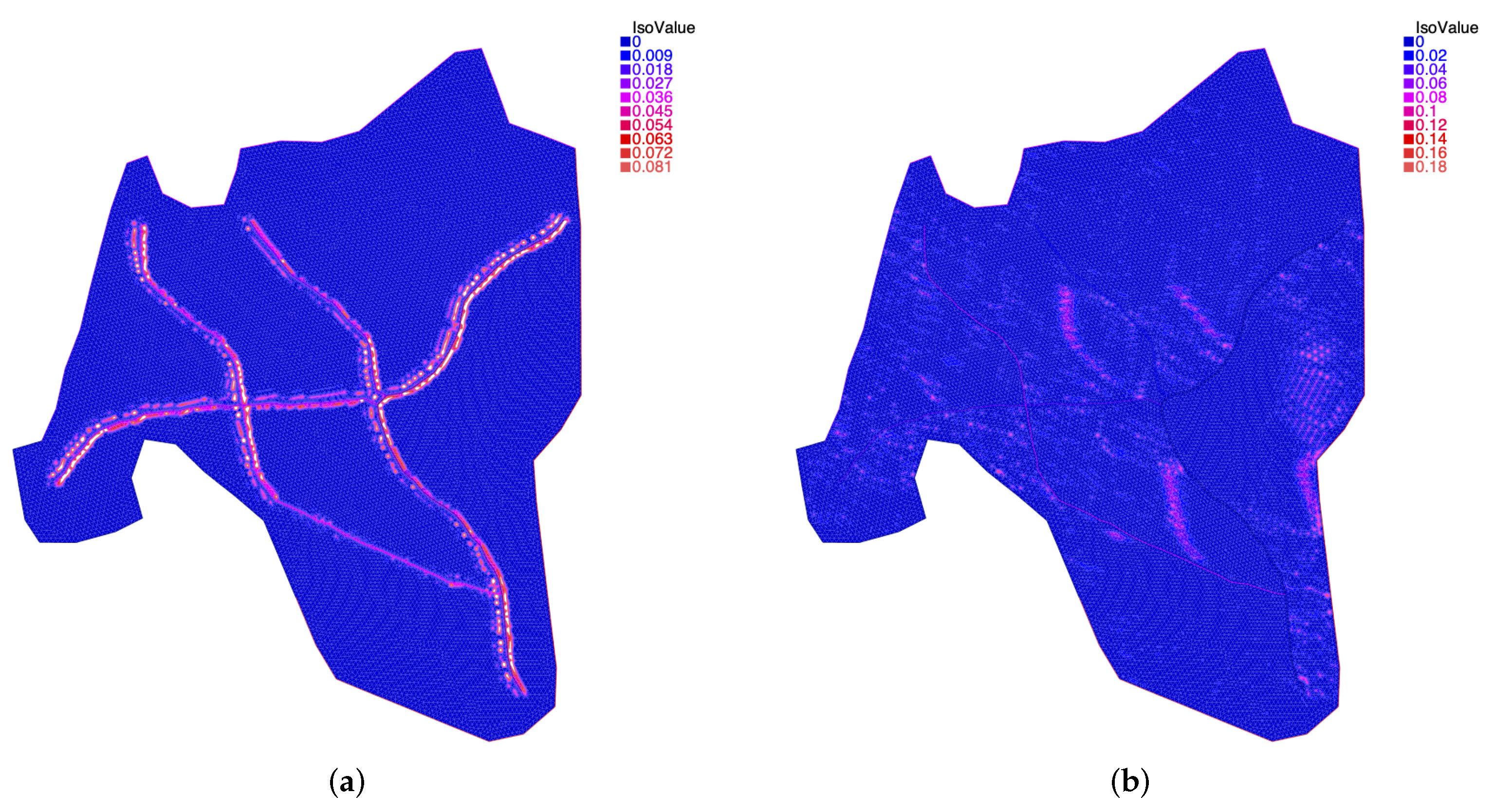
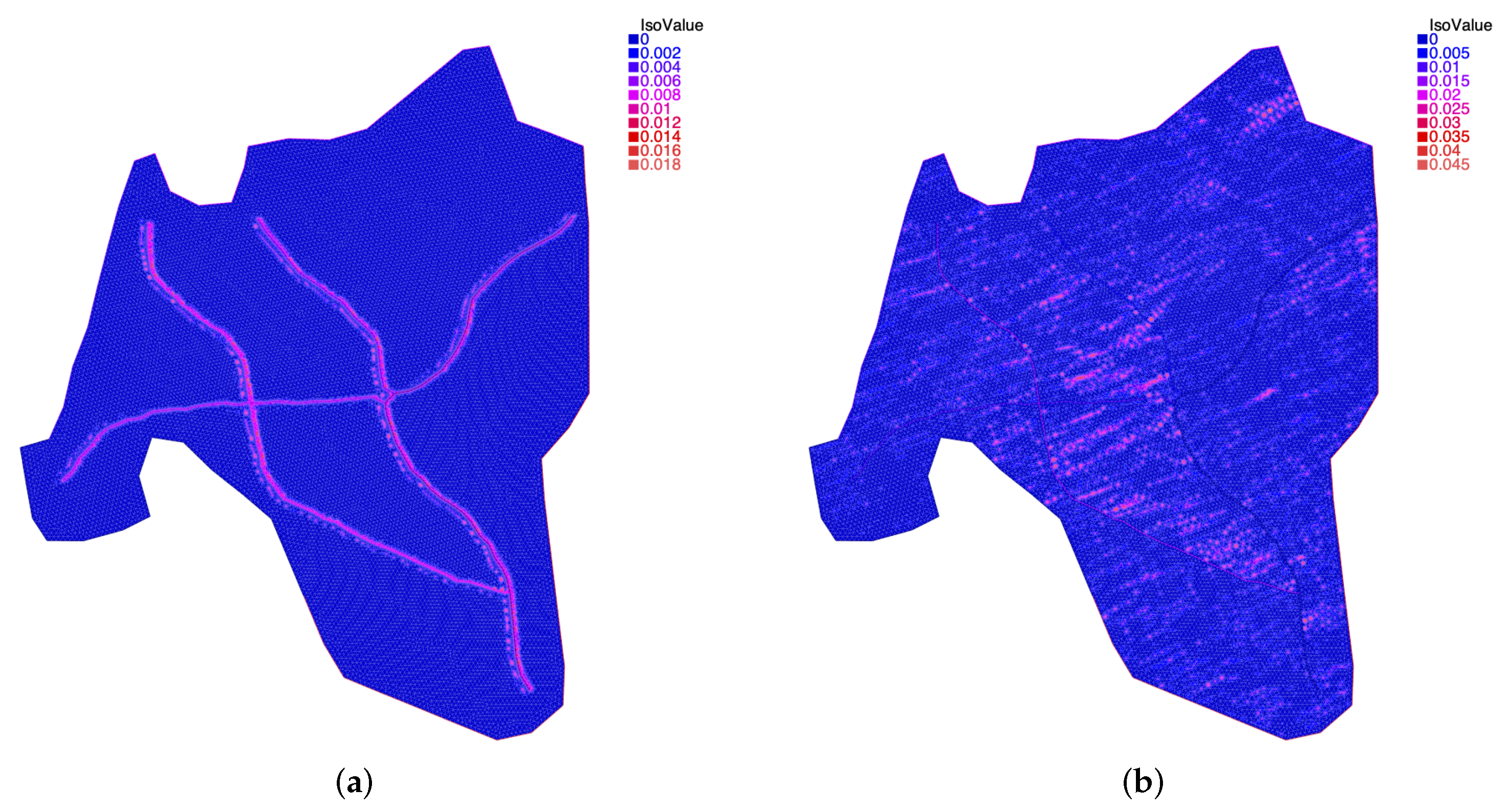
The partial concentrations of CO and PM obtained from numerical simulations from 7 a.m. to 11 a.m. of 15 May 2020 are plotted in Figure 7 and Figure 8, respectively.
In Figure 7a and Figure 8a, we observe that the CO and PM are clearly concentrated around the main traffic roads. This is due to the fact that the wind advection and diffusion are not yet sufficiently concretized since the simulation had just started. In contrast, after four hours of simulation, we observe in Figure 7b and Figure 8b a continuous propagation of CO and PM in the computational domain. This is the result of a sustained wind action and a constant increase in the number of vehicles in the traffic.
These results support that, despite the area of Bamako (about 267 km) and the low diffusion coefficients of the air pollutants studied in this framework, it only took an average of four hours during peak-period traffic congestion for these pollutants to spread over a large part of the city depending on the meteorological conditions.
The results presented in the Figures above appear promising; however, comparison studies with the data from the observations are needed for their validation, see Section 6.
6. Numerical Validation
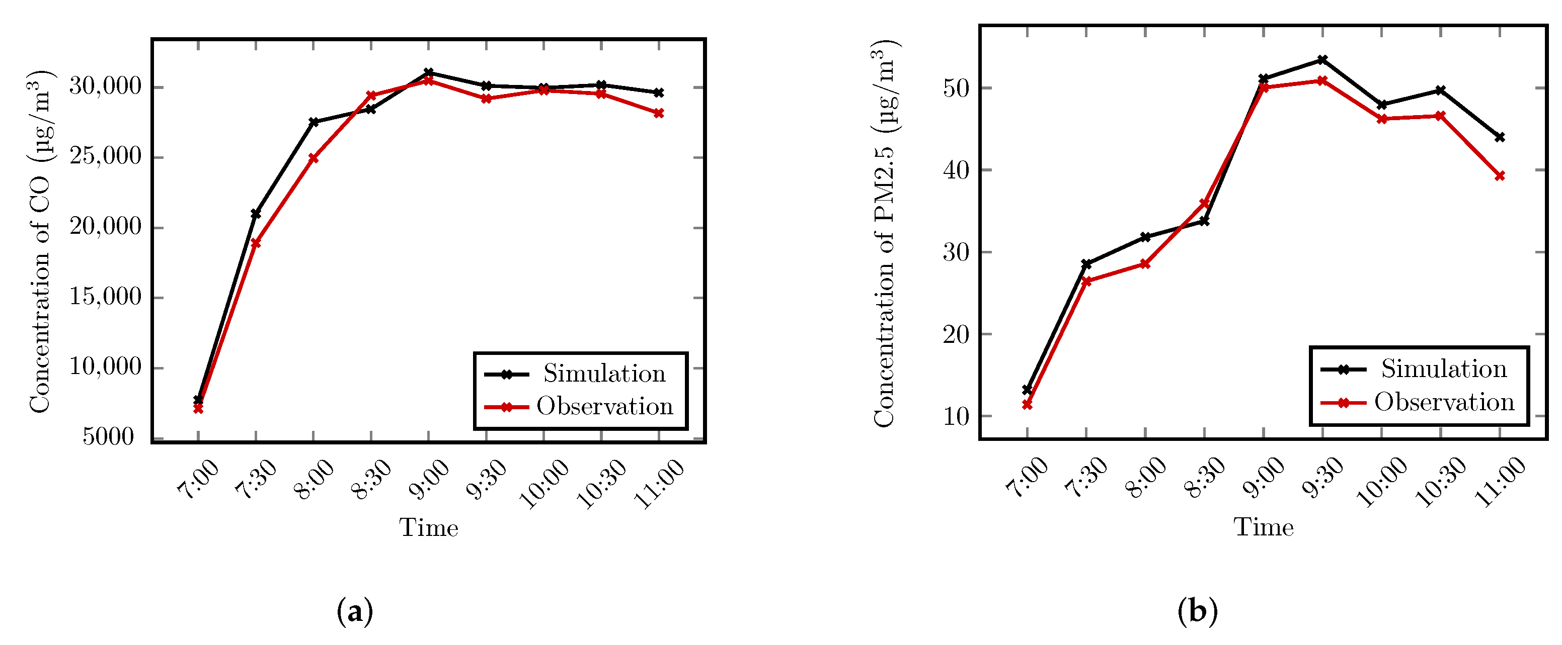
This section aims to evaluate the accuracy and validity of the numerical simulation results presented in Figure 7a and Figure 8a using observational data. For this purpose, we focused on one of the most frequented traffic roundabouts of Bamako, commonly called “independence monument”, during peak hours. The concentrations of the pollutants of interest were sampled and recorded every thirty minutes at this discrete point of the computational domain using a mobile air quality sensor. The concentrations of CO and PM from numerical simulation and observations on 15 May 2020 for the period from 7 a.m. to 11 a.m. are plotted in Figure 9a,b, respectively. Through a qualitative analysis of these figures, we can observe that, despite some simplifying assumptions in the continuous model, the simulation results are consistent with observational data since the trends of the different concentrations are similar over the period we considered.
7. Conclusions
In this paper, we presented a mathematical and numerical framework for traffic-induced air pollution simulation in Bamako, the capital of Mali. The chemical transport model that governs the spatio-temporal dynamics of the concentrations of air pollutants has been described. The initial and boundary conditions, the deposits and the chemical kinetics of the pollutants have also been presented. The traffic simulations on the main and most frequented roads of the city of Bamako were carried out using a road traffic simulation package called SUMO. The numerical simulations have been focused on the carbon monoxide (CO) and the fine particulate matter (PM). The numerical results presented here are being promising and consistent with the observational data as evidenced by the numerical validation study. These results support that the proposed framework is well suited for reproducing the spatio-temporal dynamics of the pollutants specified.
The numerical results presented in this framework were obtained using wind data of 10 spatial resolution from the European Centre for Medium-Range Weather Forecasts (ECMWF). In order to improve the model accuracy and capture more spatial information, it would be important to perform numerical simulations at higher spatial resolution, i.e., 5 or less. For that purpose, the meteorological data, especially the wind velocity fields, of similar resolution will be required. Unfortunately, we have not been able to obtain data at such a resolution from the meteorological data sources we used so far, including the ECMWF. To overcome these difficulties related to accessing high-resolution wind data, two approaches could be explored in the future. The first one involves computing the wind velocity as solution of the Reynolds-averaged Navier–Stokes (RANS) equations, which will be coupled with the reactive dispersion equation. The second approach focuses on the use of a downscaling technique to capture finer-scaled wind velocity.
The extension of this work to secondary pollutants and the processing of the chemical reactions resulting from the interactions between them in the atmosphere will be considered in the near future.
Author Contributions
Conceptualization, A.S. and A.M.; methodology, A.S., A.M. and M.A.; software, A.S., A.M. and M.A.; validation, A.S., A.M., M.A. and O.D.; writing—original draft preparation, A.S.; writing—review and editing, A.S.; supervision, O.D.; project administration, O.D.; funding acquisition, A.S, A.M., M.A. and O.D. All authors have read and agreed to the published version of the manuscript.
Funding
This work was Partially funded by the Rectorate of the University of Sciences, Techniques and Technologies of Bamako (USTTB).
Institutional Review Board Statement
Not applicable.
Informed Consent Statement
Not applicable.
Data Availability Statement
The wind data used in the article are obtained from the European Centre for Medium-Range Weather Forecasts (ECMWF). They can be made available upon request.
Acknowledgments
The authors would like to acknowledge the high-performance computing support from the “Centre de Calcul, Modélisation et Simulation” (CCMS) of the Faculty of Sciences and Technology (FST) of Bamako.
Conflicts of Interest
The authors declare no conflict of interest.
References
- Jorquera, H.; Montoya, L.D.; Rojas, N.Y. Urban Air Pollution. In Urban Climates in Latin America; Henríquez, C., Romero, H., Eds.; Springer International Publishing: Cham, Switzerland, 2019; pp. 137–165. [Google Scholar] [CrossRef]
- World Health Organization. Air pollution. 2020. [Google Scholar]
- World Health Organization. Outdoor air pollution a leading environmental cause of cancer deaths. IARC Sci Publ 2013, 161, 1–177. [Google Scholar]
- Karroum, K.; Lin, Y.; Chiang, Y.Y.; Ben Maissa, Y.; El Haziti, M.; Sokolov, A.; Delbarre, H. A review of air quality modeling. MAPAN 2020, 35, 287–300. [Google Scholar] [CrossRef]
- Leelossy, Á.; Molnár, F.; Izsák, F.; Havasi, Á.; Lagzi, I.; Mészáros, R. Dispersion modeling of air pollutants in the atmosphere: A review. Open Geosci. 2014, 6, 257–278. [Google Scholar] [CrossRef]
- Mallet, V.; Sportisse, B. Air quality modeling: From deterministic to stochastic approaches. Comput. Math. Appl. 2008, 55, 2329–2337. [Google Scholar] [CrossRef]
- Leelossy, Á.; Mona, T.; Mészáros, R.; Lagzi, I.; Havasi, Á. Eulerian and Lagrangian approaches for modelling of air quality. In Mathematical Problems in Meteorological Modelling; Springer: Cham, Switzerland, 2016; pp. 73–85. [Google Scholar]
- INSTAT-ML. Annuaire Statistique du Mali; Technical Report; Institut National de la Statistique (MALI): Bamako, Mali, 2018. [Google Scholar]
- Fallah-Shorshani, M.; Shekarrizfard, M.; Hatzopoulou, M. Evaluation of regional and local atmospheric dispersion models for the analysis of traffic-related air pollution in urban areas. Atmos. Environ. 2017, 167, 270–282. [Google Scholar] [CrossRef]
- AGRECO, C. Révision du Profil Environnemental du Mali; Technical Report; European Union: Brussels, Belgium, 2014. [Google Scholar]
- World Health Organization. WHO Global Air Quality Guidelines: Particulate Matter (PM2.5 and PM10), Ozone, Nitroge n Dioxide, Sulfur Dioxide and Carbon Monoxide; World Health Organization: Geneva, Switzerland, 2021. [Google Scholar]
- Samaké, A.; Mahamane, A.; Diallo, O. Parallel Implementation and Scalability Results of a Local-scale Air Quality Model: Application to Bamako Urban City. J. Appl. Math. 2022, 2022, 9463537. [Google Scholar] [CrossRef]
- Keïta, M. Typologie urbaine et accessibilité géographique potentielle des établissements de santé dits «modernes» dans le district de Bamako (Mali). Espace Popul. Soc. 2018, 2018, 1–2. [Google Scholar] [CrossRef]
- Mukim, M. Bamako Urban Sector Review: An Engine of Growth and Service Delivery; Technical Report; The World Bank: Washington, DC, USA, 2018. [Google Scholar]
- Sportisse, B. Fundamentals in Air Pollution: From Processes to Modelling; Springer Science & Business Media: Dordrecht, The Netherlands, 2009. [Google Scholar]
- Hu, X.M. Boundary Layer (Atmospheric) and Air Pollution | Air Pollution Meteorology. In Encyclopedia of Atmospheric Sciences, 2nd ed.; North, G.R., Pyle, J., Zhang, F., Eds.; Academic Press: Oxford, UK, 2015; pp. 227–236. [Google Scholar] [CrossRef]
- Seinfeld, J.H.; Pandis, S.N. Atmospheric Chemistry and Physics: From Air Pollution to Climate Change; John Wiley & Sons: Hoboken, NJ, USA, 2016. [Google Scholar]
- Giardina, M.; Buffa, P. A new approach for modeling dry deposition velocity of particles. Atmos. Environ. 2018, 180, 11–22. [Google Scholar] [CrossRef]
- Sportisse, B. A review of parameterizations for modelling dry deposition and scavenging of radionuclides. Atmos. Environ. 2007, 41, 2683–2698. [Google Scholar] [CrossRef]
- Youngseob, K. Modélisation de la Qualité de l’Air: Évaluation des Paramétrisations Chimiques et Météorologiques. Ph.D. Thesis, Université Paris-Est, Marne-la-Vallée, France, 2011. [Google Scholar]
- Sportisse, B. A review of current issues in air pollution modeling and simulation. Comput. Geosci. 2007, 11, 159–181. [Google Scholar] [CrossRef]
- Goeke, A.; Walcher, S. A constructive approach to quasi-steady state reductions. J. Math. Chem. 2014, 52, 2596–2626. [Google Scholar] [CrossRef]
- Mooney, P. An Outlook for OpenStreetMap. In OpenStreetMap in GIScience: Experiences, Research, and Applications; Jokar Arsanjani, J., Zipf, A., Mooney, P., Helbich, M., Eds.; Springer International Publishing: Cham, Switzerland, 2015; pp. 319–324. [Google Scholar] [CrossRef]
- Vandecasteele, A.; Devillers, R. Improving Volunteered Geographic Information Quality Using a Tag Recommender System: The Case of OpenStreetMap. In OpenStreetMap in GIScience: Experiences, Research, and Applications; Jokar Arsanjani, J., Zipf, A., Mooney, P., Helbich, M., Eds.; Springer International Publishing: Cham, Switzerland, 2015; pp. 59–80. [Google Scholar] [CrossRef]
- QGIS Development Team. QGIS Geographic Information System; QGIS Association: Zurich, Switzerland, 2022. [Google Scholar]
- Geuzaine, C.; Remacle, J.F. Gmsh: A 3-D finite element mesh generator with built-in pre-and post-processing facilities. Int. J. Numer. Methods Eng. 2009, 79, 1309–1331. [Google Scholar] [CrossRef]
- Barceló, J. Fundamentals of traffic simulation; Springer: New York, NY, USA, 2010; Volume 145. [Google Scholar]
- Lopez, P.A.; Behrisch, M.; Bieker-Walz, L.; Erdmann, J.; Flötteröd, Y.P.; Hilbrich, R.; Lücken, L.; Rummel, J.; Wagner, P.; WieBner, E. Microscopic traffic simulation using sumo. In Proceedings of the 2018 21st International Conference on Intelligent Transportation Systems (ITSC), Maui, HI, USA, 4–7 November 2018; IEEE: Maui, HI, USA, 2018; pp. 2575–2582. [Google Scholar] [CrossRef] [Green Version]
- Behrisch, M.; Weber, M. Simulating Urban Traffic Scenarios; Springer: Cham, Switzerland, 2018. [Google Scholar]
- Chen, T.M.; Kuschner, W.G.; Gokhale, J.; Shofer, S. Outdoor air pollution: Nitrogen dioxide, sulfur dioxide, and carbon monoxide health effects. Am. J. Med. Sci. 2007, 333, 249–256. [Google Scholar] [CrossRef] [PubMed]
Figure 1.
Geographical location and politico-administrative division of Bamako. Source: [13].
Figure 1.
Geographical location and politico-administrative division of Bamako. Source: [13].

Figure 2.
Urban area delimitation and road traffic network of Bamako. Source: [14].
Figure 2.
Urban area delimitation and road traffic network of Bamako. Source: [14].

Figure 3.
Daily mean PM concentration in Bamako over October 2020. Data source: World Air Quality Index (WAQI) Project database 2020—U.S. Environmental Protection Agency.
Figure 3.
Daily mean PM concentration in Bamako over October 2020. Data source: World Air Quality Index (WAQI) Project database 2020—U.S. Environmental Protection Agency.

Figure 4.
Monthly mean PM concentration in Bamako over the period from January to November 2020. Data source: World Air Quality Index (WAQI) Project database 2020—U.S. Environmental Protection Agency.
Figure 4.
Monthly mean PM concentration in Bamako over the period from January to November 2020. Data source: World Air Quality Index (WAQI) Project database 2020—U.S. Environmental Protection Agency.

Figure 5.
Three-dimensional computational domain of Bamako and traffic roads. (a) Three-dimensional domain of Bamako. View on upper limit and lateral boundaries. (b) Three-dimensional domain of Bamako. View on the ground boundary with roads. Source: [12].
Figure 5.
Three-dimensional computational domain of Bamako and traffic roads. (a) Three-dimensional domain of Bamako. View on upper limit and lateral boundaries. (b) Three-dimensional domain of Bamako. View on the ground boundary with roads. Source: [12].

Figure 6.
Three-dimensional computational mesh and two-dimensional mesh of the ground. (a) Three-dimensional mesh from the computational domain Figure 5a. (b) Mesh of the ground boundary extracted from three-dimensional mesh. Source: [12].

Figure 7.
Spatial concentrations of CO in Bamako on 15 May 2020 at 7 a.m. and 11 a.m. (a) Spatial concentration of CO (g/m) from the road traffic on 15 May 2020 at 7 a.m. (b) Spatial concentration of CO (g/m) from the road traffic on 15 May 2020 at 11 a.m.
Figure 7.
Spatial concentrations of CO in Bamako on 15 May 2020 at 7 a.m. and 11 a.m. (a) Spatial concentration of CO (g/m) from the road traffic on 15 May 2020 at 7 a.m. (b) Spatial concentration of CO (g/m) from the road traffic on 15 May 2020 at 11 a.m.

Figure 8.
Spatial distribution of PM in Bamako on 15 May 2020 at 7 a.m. and 11 a.m. (a) Spatial distribution of PM (mg/m) from the road traffic on 15 May 2020 at 7 a.m. (b) Spatial distribution of PM (mg/m) from the road traffic on 15 May 2020 at 11 a.m.
Figure 8.
Spatial distribution of PM in Bamako on 15 May 2020 at 7 a.m. and 11 a.m. (a) Spatial distribution of PM (mg/m) from the road traffic on 15 May 2020 at 7 a.m. (b) Spatial distribution of PM (mg/m) from the road traffic on 15 May 2020 at 11 a.m.

Figure 9.
Concentration of CO and PM from simulation and observation on 15 May 2020. (a) Concentration of CO from simulation and observation on 15 May 2020. (b) Concentration of PM from simulation and observation on 15 May 2020.
Figure 9.
Concentration of CO and PM from simulation and observation on 15 May 2020. (a) Concentration of CO from simulation and observation on 15 May 2020. (b) Concentration of PM from simulation and observation on 15 May 2020.


| Symbol | Name | Unit |
|---|---|---|
| c | concentration | kg m |
| wind velocity | m s | |
| diffusion coefficient | m s | |
| deposition velocity | m s | |
| scavenging coefficient | s | |
| chemical sources | kg m s | |
| S | volume emissions | kg m s |
| E | surface emissions | kg m s |
| H | maximum altitude | m |
| characteristic time | s |
Publisher’s Note: MDPI stays neutral with regard to jurisdictional claims in published maps and institutional affiliations. |
© 2022 by the authors. Licensee MDPI, Basel, Switzerland. This article is an open access article distributed under the terms and conditions of the Creative Commons Attribution (CC BY) license (https://creativecommons.org/licenses/by/4.0/).
Share and Cite
MDPI and ACS Style
Samaké, A.; Mahamane, A.; Alassane, M.; Diallo, O. A Mathematical and Numerical Framework for Traffic-Induced Air Pollution Simulation in Bamako. Computation 2022, 10, 76. https://0-doi-org.brum.beds.ac.uk/10.3390/computation10050076
AMA Style
Samaké A, Mahamane A, Alassane M, Diallo O. A Mathematical and Numerical Framework for Traffic-Induced Air Pollution Simulation in Bamako. Computation. 2022; 10(5):76. https://0-doi-org.brum.beds.ac.uk/10.3390/computation10050076
Chicago/Turabian StyleSamaké, Abdoulaye, Amadou Mahamane, Mahamadou Alassane, and Ouaténi Diallo. 2022. "A Mathematical and Numerical Framework for Traffic-Induced Air Pollution Simulation in Bamako" Computation 10, no. 5: 76. https://0-doi-org.brum.beds.ac.uk/10.3390/computation10050076
Note that from the first issue of 2016, this journal uses article numbers instead of page numbers. See further details here.