Bullet Frangibility Factor Quantification by Using Explicit Dynamic Simulation Method

Abstract

Frangible bullets have a unique property that disintegrates into fragments upon hitting a hard target or obstacle. This peculiar ability to become fragments after impact is called frangibility. In this study, frangibility testing was carried out theoretically via modeling using the explicit dynamics method with ANSYS Autodyn solver integrated by ANSYS Workbench software. This paper aims to analyze frangibility through two main factors: material properties and projectile design. The results show the scattering and remaining bullet fragments after impact. According to the modeling results, the frangibility factor values are 9.34 and 10.79, respectively. Based on the frangibility factor, errors based on the frangibility factor by comparing the experimental results and simulations for AMMO 1 and AMMO 2 are 10.5% and 1.09%. Based on simulation results, the AMMO 2 design bullet scattering pattern shows several scattering particles more than the AMMO 1 design, with the furthest distance scattering AMMO 1 and AMMO 2 bullets being 1.01 m and 2658 m.

1. Introduction

The frangible bullet has become one of the breakthroughs in the defense sector due to their fragmentation ability upon impact on a hard target [1]. This disintegration ability makes frangible bullets uniquely different from conventional bullets, minimizing the ricochet and backsplash phenomenon [2,3]. The frangibility factor is the most crucial feature that a frangible bullet must possess from a ballistic perspective. Frangibility quantification has a high practical value in evaluating bullet fragmentation capability, and it is needed to conduct a ballistic experiment in several method variations, whether theoretical or practical [3,4]. Recently, frangibility quantification involving an actual experiment has been producing the highest and most accurate data results. However, this method has many difficulties, including relatively high cost, requiring advanced instruments, and needing a relatively long duration to achieve precise accuracy [5].

Additionally, parameters that affect the ballistic test result also face many difficulties due to their dynamic response to the environment, including the shooter condition. A more straightforward solution provided in terms of time and cost is by using a theoretical method that utilizes numerical calculation and finite element simulation. However, theoretical approaches and simulation tend to be more complex than a conventional experiment, and this method is rarely used and developed globally [5,6,7].

Previously, there was frangibility factor quantification research that was done by using numerical and simulation methods. Amrullah et al. conducted an impact simulation of a copper-tin metal matrix composite frangible bullet on a hard target using smoothed particle hydrodynamics [8]. This simulation result did not show an exact quantification of the frangibility properties. Moreover, this method could not show the after-impact condition of the frangible bullet, which is necessary for frangibility factor consideration [8]. On the other hand, a smoothed particle hydrodynamic simulation conducted by Simarmare also could not show the scattering pattern of the frangible bullet upon impact, which could not be used for further calculation [9].

To achieve well-visualized modeling results which are close to the actual experiment, theoretical frangibility quantification analysis can be done by explicit dynamics method using ANSYS Workbench. Using this Autodyn integrated simulation, frangibility factor quantification could be simpler and faster. Moreover, using this method, supporting data for calculation that is impossible to extract during the actual experiment can be achieved, which could be a better prospect in calculating the frangibility factor of a bullet without experimenting with actual ballistic testing [7,10,11,12,13,14,15].

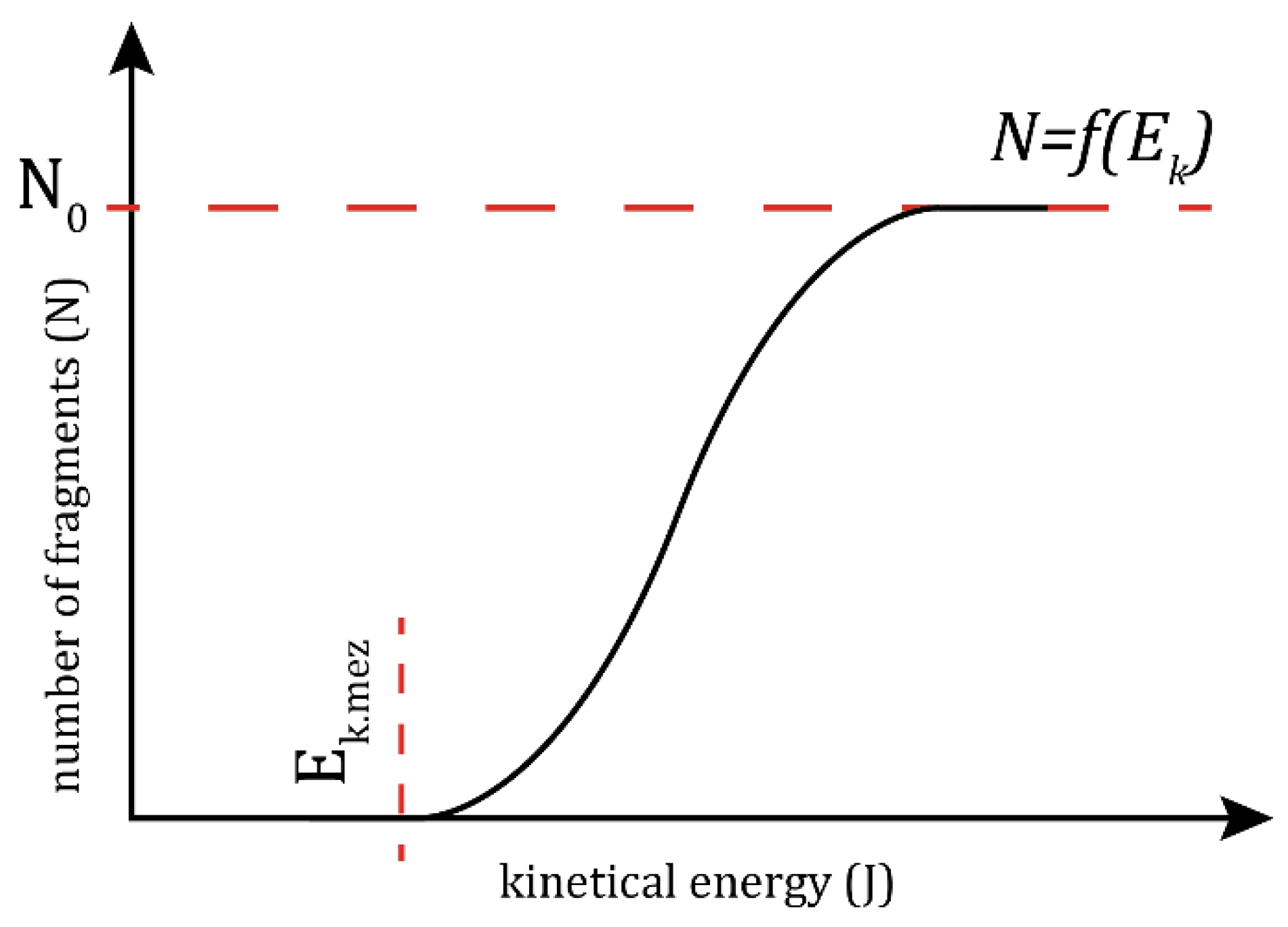
Ballistic testing consists of many subdisciplines, including frangibility testing. Frangibility, the most crucial property in determining a frangible bullet, is the ability of a material to disintegrate upon hitting a hard target [16,17]. Several factors have a considerable influence on determining the frangibility factor of a bullet, including base materials, mechanical properties, targeted object, and impact condition in the form of kinetical energy. Frangibility also affects the fragmentation size, so that a high frangibility factor material has finer fragments after the impact which is illustrated in Figure 1 [1].

Theoretically, frangibility can be evaluated by calculating the frangibility factor. Frangibility factor (FF_T) is defined as the ratio between kinetical energy (E_k) at the first impact stage and the lowest limit of the kinetical energy (E_k,lim) [5]. The frangibility factor can be expressed as the following equation:

$$F{F}_T=\frac{E_k}{E_{k,lim}}$$

(1)

Kinetical energy upon impact can be defined using the following standard energy equation:

$$E_k=\frac{1}{2}{m}_q{v}_{imp}^2$$

(2)

where $m_q$ is the mass and $v_{imp}$ is the impact velocity of the projectile. At the same time, the following formula is used to calculate the kinetical energy limit [5].

$$E_{k,lim}=\frac{1}{2}{m}_q{v}_{k,lim}^2$$

(3)

The bullet velocity impact ($v_{k,\mathit{lim}})$ value depends on the target material mechanical properties. This velocity shows the maximum value of bullet speed on a defined target where for the materials the fragmentation has still not taken place. Still, a crack can be formed on the projectile body. The impact velocity limit of the bullet can be formulated as follows:

$$v_{k,lim}=\frac{2K{\epsilon }_{x,max}}{\rho l}\sqrt{m_q\left(\frac{4l}{3K\pi d^2}+\frac{1}{c}\right)}$$

(4)

where K, ${\epsilon }_{x,max}$, $\rho$, $l$, and d are the projectile elastic modulus, maximal compressive strain, density, length, and diameter, respectively, whilst c is the target hardness value in N/m. A projectile is considered as frangible if its FF_T value is greater than 1 and if its FF_T value is less than 1; the projectile cannot therefore disintegrate upon impact [5].

Generally, material testing consists of two main methods: static and dynamic. In the static method, a non-moving sample is given an external force to perform the testing. In contrast, in a dynamic way, the testing is carried out with a moving model, which results in an internal pressure [18]. In this paper, frangibility testing is focused on the bullet performance during the firing stage, so the dynamic method is used for this research. Based on the time integration used during the simulation process, there are two sub-methods applied in the material modeling; namely, implicit and explicit dynamic. Implicit dynamics tend to have a longer integration time, which means that a modeled material failure case must have a longer time to take place, such as creep, static structural, or a quasi-static model. On the other hand, explicit dynamics solve a relatively slower time integration (within a microsecond) for a material failure phenomenon. Usually, this sub-method is used for determining the dynamic response of a structural material subjected to shockwave propagation, large deformation and strain, non-linear material behavior, fragmentation, or non-linear buckling. To identify the dynamic simulation performance of frangible bullets, an explicit dynamic sub-method is utilized during the simulation process [19].

The explicit method used in the explicit dynamic analysis is based on the half-step major differences, which are shown in the following equation [20]:

$${\ddot{D}}_n=\frac{{\dot{D}}_{n+\frac{1}{2} }-{\dot{D}}_{n-\frac{1}{2}}}{∆t} \mathrm{or} {\dot{D}}_{n+\frac{1}{2} }={\dot{D}}_{n-\frac{1}{2}}+{\ddot{D}}_n∆t$$

(5)

$${\dot{D}}_{n+\frac{1}{2}}=\frac{D_{n+1 }-D_n}{∆t} \mathrm{or} D_{n+1 }=D_n+{\dot{D}}_{n+\frac{1}{2}} ∆t$$

(6)

Equations (5) and (6) are the explicit method formula because the calculation of ${\dot{D}}_{n+\frac{1}{2}}$ and $D_{n+1}$ only require data from the historical response during formulation. With this equation, time response can be calculated explicitly without using the iteration of the time step, which leads to the increasing of the cycle efficiency. The highlighted characteristic of the explicit dynamic is that this method requires a very small integration of the time step to achieve precise solutions [20].

The 3D design of the bodies used for the explicit dynamic analysis system is illustrated in Figure 2. It begins with cycle, displacement ($D_{n }$), and the velocity ${\ddot{D}}_n$ from the cycle which has been determined, and with this determined parameters, strain and strain rate could be calculated on each element. Volume change for each element is then calculated, which is then later used as the volumetric data that determine the stress of each element. The stress is integrated with the body of a simulated part, and the external load is input to form the nodal force $F_n$ [20]. Then, the nodal acceleration is calculated using the following equation:

$${\ddot{D}}_n=\frac{F_n}{m}+\frac{b}{\rho }$$

(7)

With this explicit method, the time integration type that is used is in the scale of nanosecond to microsecond. If this method is used during millisecond to second, then the required integration time could consist of up to a thousand or even one million cycles. Explicit dynamic method is really useful if utilized on a high velocity impact case such as frangibility testing and non-linear modelling. If used for a longer integration time, this method is less efficient and perhaps not even suitable because it requires a longer computational time [20].

2. Materials and Methods

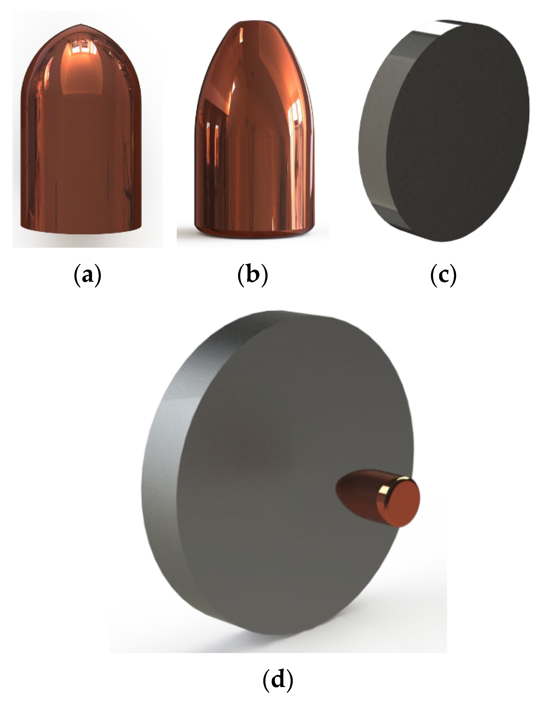
In this section, material properties will be used as the main input for engineering data in ANSYS that define the simulation part properties. The first design of the frangible bullet (AMMO 1) was used by Firmansya et al. in a real firing experiment to determine the frangibility factor of the bullet [21]. The mechanical and dynamic properties of AMMO 1 are shown in

Table 1. AMMO 1 specification.

Specification	Value
Base material	Cu-10 wt% Sn
Projectile mass (gr)	6.12
Projectile density (kg/m3)	7700
Elastic modulus (MPa)	54,383.9
Poisson’s Ratio	0.3
Bulk Modulus (MPa)	45,320
Shear Modulus (MPa)	20,917
Kinetical energy limit (Joule)	39.56
Frangibility factor	9.34
Kinetical energy at 2 m away from gun barrel (Joule)	368.79

.

For the second projectile design (AMMO 2), experimental data from Mia et al. is used, shown in the

Table 2. AMMO 2 spesification.

Specification	Value
Base material	Cu-10%Sn
Projectile mass (gr)	5.23
Projectile density (kg/m3)	6607.46
Elastic modulus (MPa)	53,331.63
Poisson’s Ratio	0.3
Bulk Modulus (MPa)	44,443
Shear Modulus (MPa)	20,512
Kinetical energy limit (Joule)	33.67
Frangibility factor	10.91
Kinetical energy at 2 m away from gun barrel (Joule)	267.33

.

Where $v_t$ is velocity at 0 m from target, $v_0$ is the initial velocity, $a$ is the projectile acceleration, and S is the travel distance of the projectile.

According to the ballistic standard, ST37 Steel is used as the target’s base material. Nevertheless, this steel type is not common and is recently being used less as the target shooting material. Hence, another type of steel with equivalent mechanical properties is now utilized, which is ASTM A36 Mild Steel. The mechanical properties of this steel are shown in the

Table 3. Steel plate mechanical properties.

Specification	Value
Base material	ASTM A36 Mild Steel
Density (g/cm3)	7.85
Yield strength (MPa)	250
Young modulus (GPa)	210
Poisson Ratio	0.26
Frangibility factor	10.91
Geometry shape	Solid cylinder
Diameter (mm)	600
Thickness (mm)	20

.

To reduce time needed for simulation, during the simulation part assembly process, the distance between projectile and target is set to 10 mm apart. Due to this condition, initial velocity of the projectile is manually calculated by using the linear motion equation of accelerated particles as follows:

$$v_t{}^2=v_0{}^2+2aS$$

(8)

Based on the research team’s actual firing experiment of the frangible bullet, initial velocity of the projectile after leaving the gun barrel is used to calculate the velocity at a desired position from the target. With the calculated velocity, kinetical energy formulation at 10 mm apart from the firing target can be carried out by using the following equation:

$$E_k=\raisebox{1ex}{$1$}\!\left/ \!\raisebox{-1ex}{$2$}\right.m_p{v}_x{}^2$$

(9)

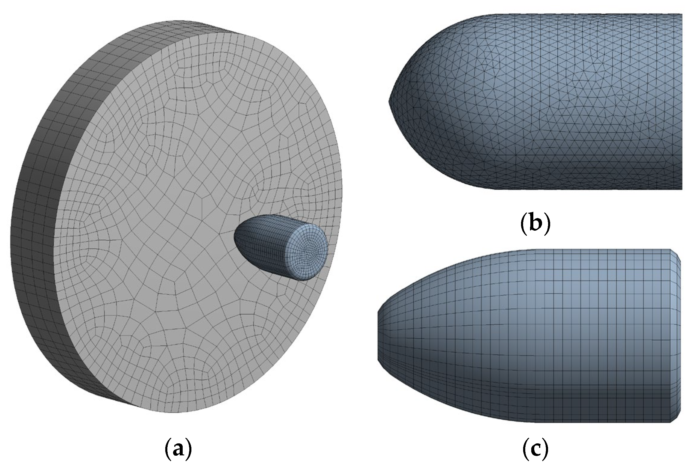
Before starting the simulation process, choosing the right element size and meshing type is a considerable aspect to achieve a precise modelling result. In this paper, automatic meshing with 0.5 mm is used to determine the bullet body part. With the automatic method, the system will decide the most effective meshing shape for a certain geometry. The simulation used the automatic method so the shape of the elements and nodes can be varied depending on the complexity of the geometry. For AMMO 1, due to its sharp bullet head, the most suitable is a triangular element mesh. On the other hand, AMMO 2 has tetrahedral shape that is generated by the automatic meshing. However, the element size used during the simulation have the same size (0.5 mm), which created a nearly similar element quantity at 59,577 elements for AMMO 1 and 59,458 elements for AMMO 2. The meshing result of AMMO 1 and AMMO 2 can be seen in Figure 3. It shows that there is a different element shape between AMMO 1, AMMO 2, and the firing plate. With the plate as fixed support (immoveable object), the simulation is carried out by inputting velocity at 10 mm before the target. In a real firing experiment, the firing distance is set to 3 m away from the plate. To perform a more efficient modelling process, 10 mm distance is chosen, but it is needed to calculate the actual velocity at 10 mm before hitting the target with a previous equation. The initial speed of the projectile is obtained by a shooting experiment that used a velocity sensor to find out the actual initial speed which presented in

Table 4. Projectile initial condition.

Parameters	AMMO 1	AMMO 2
Mass (kg)	0.00612	0.00523
Acceleration (m/s2)	30,130.02	34,969
Initial velocity (m/s)	424.47	457.29

. In the absence of an actual experiment, this velocity can be acquired in the bullet technical datasheet because every ammunition caliber has its own standard. During the actual experiment, a projectile that leaves the gun barrel has a velocity of 347.16 m/s in value. This velocity is the initial velocity ($v_0$) that will be used to calculate the acceleration of the projectile. After calculating the acceleration, then the velocity at 10 mm before hitting the target can be quantified. With an initial velocity equal to 347.16 m/s and an acceleration equal to 30,130.02 m/s², the temporary velocity at 10 mm away is equal to 424.47 m/s. This velocity will be used as an initial condition of the projectile, and the time step is set to 1.2 ms so the bullet fragmentation could be illustrated.

3. Results and Discussions

During the simulation process, the projectile is positioned by inputting the pre-determined velocity to the X-axis direction of the plate while the plate is set to be an immovable object or fixed support as the firing target. This simulation is assumed as uniform or a steady environment (without subjecting external force), and then followed by the simulation process calculation.

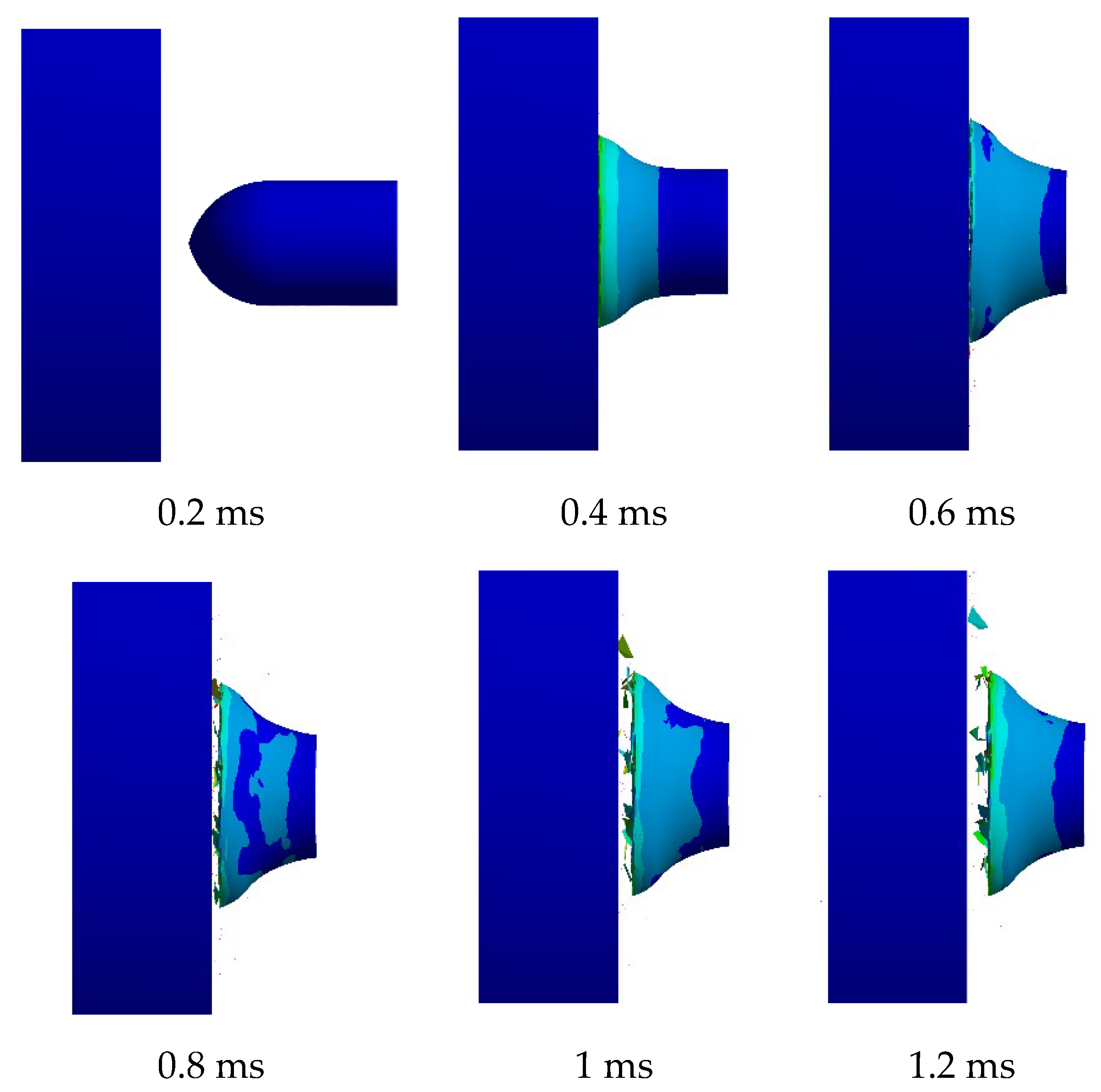
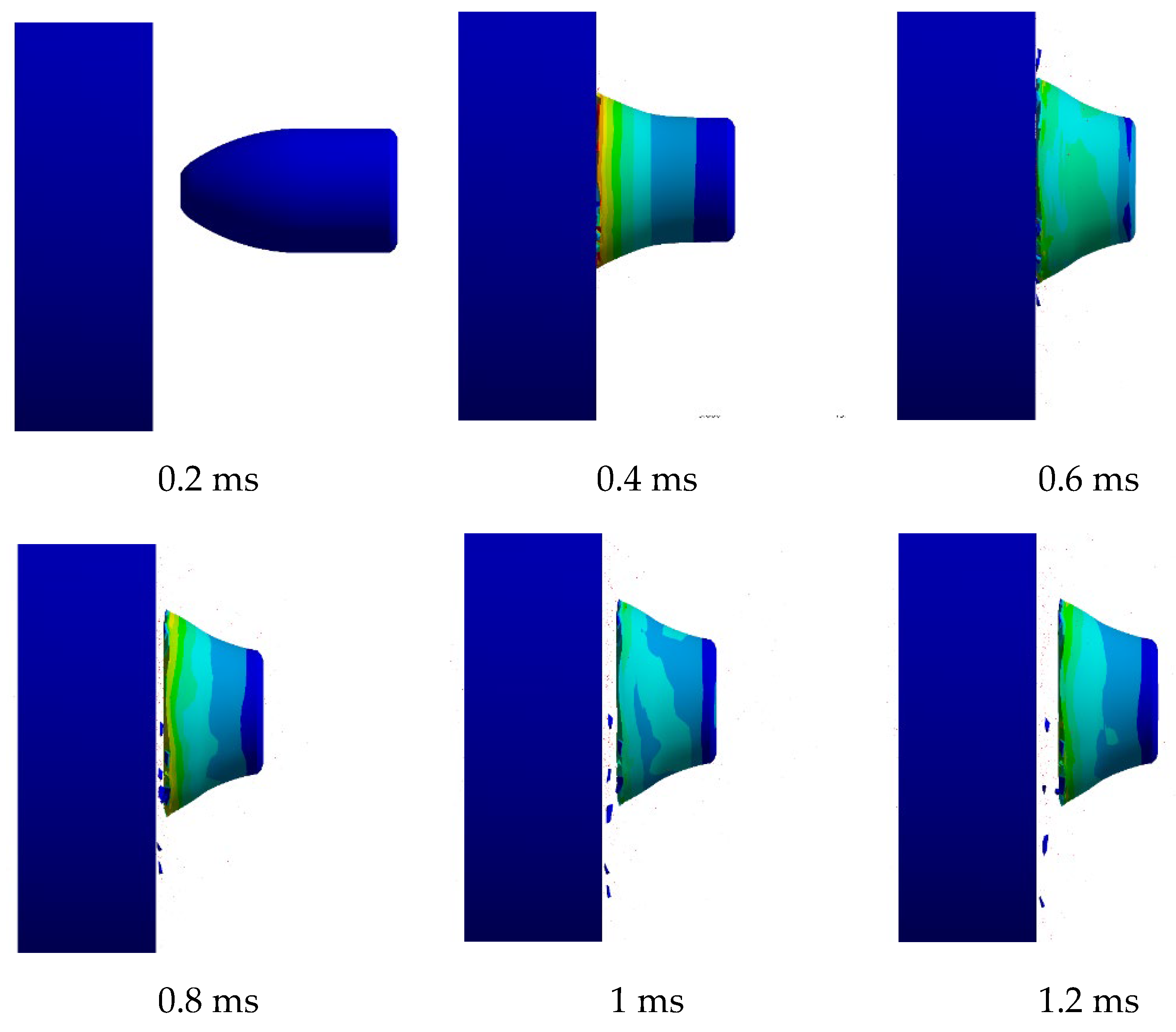
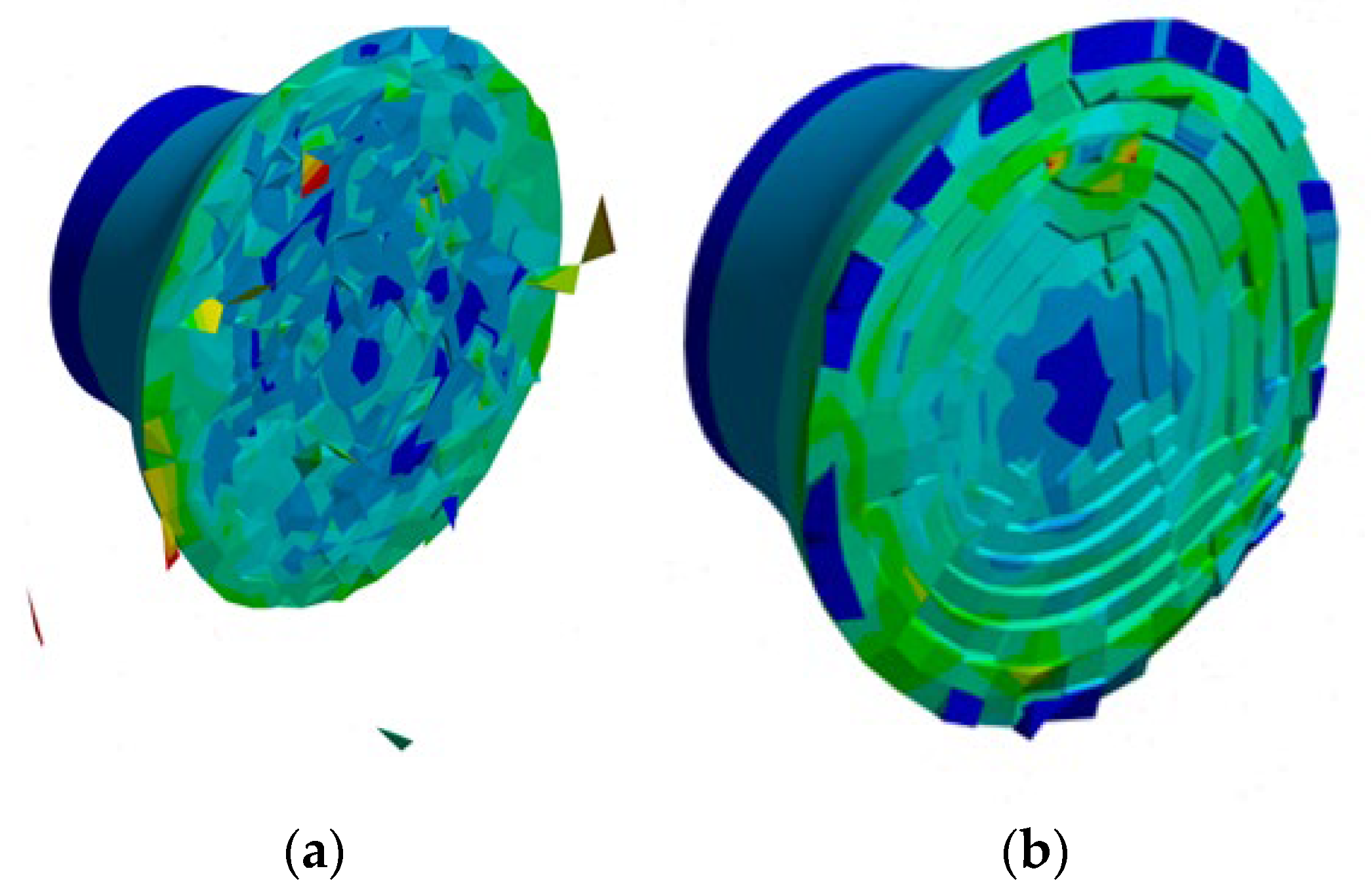
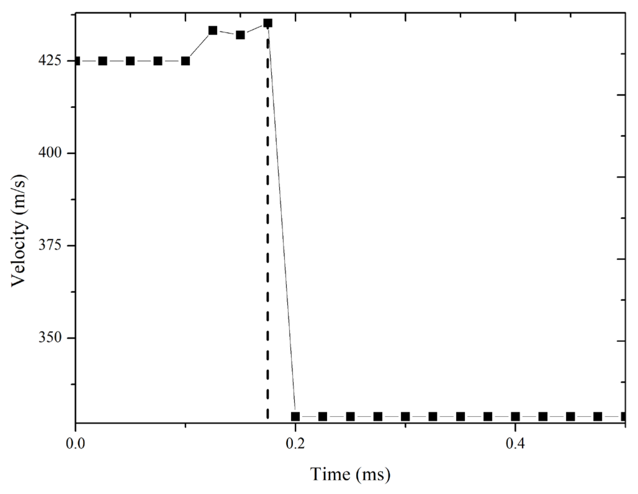
After the calculation impact simulation process, the result obtained will then show the bullet evolution from pre-impact and after impact conditions. This impact phenomenon of the projectile is presented between 0.2 to 1.2 milliseconds. Figure 4 and Figure 5 show the disintegration process and projectile evolution graph of AMMO 1 over time. Based on the figures, the projectile is disintegrated due to its lower mechanical properties compared to the steel plate. The frangible projectile has a lower hardness and toughness that lead to deformation with a high number of fragments due to its frangibility properties. The projectile initial deformation started at 0.4 ms.

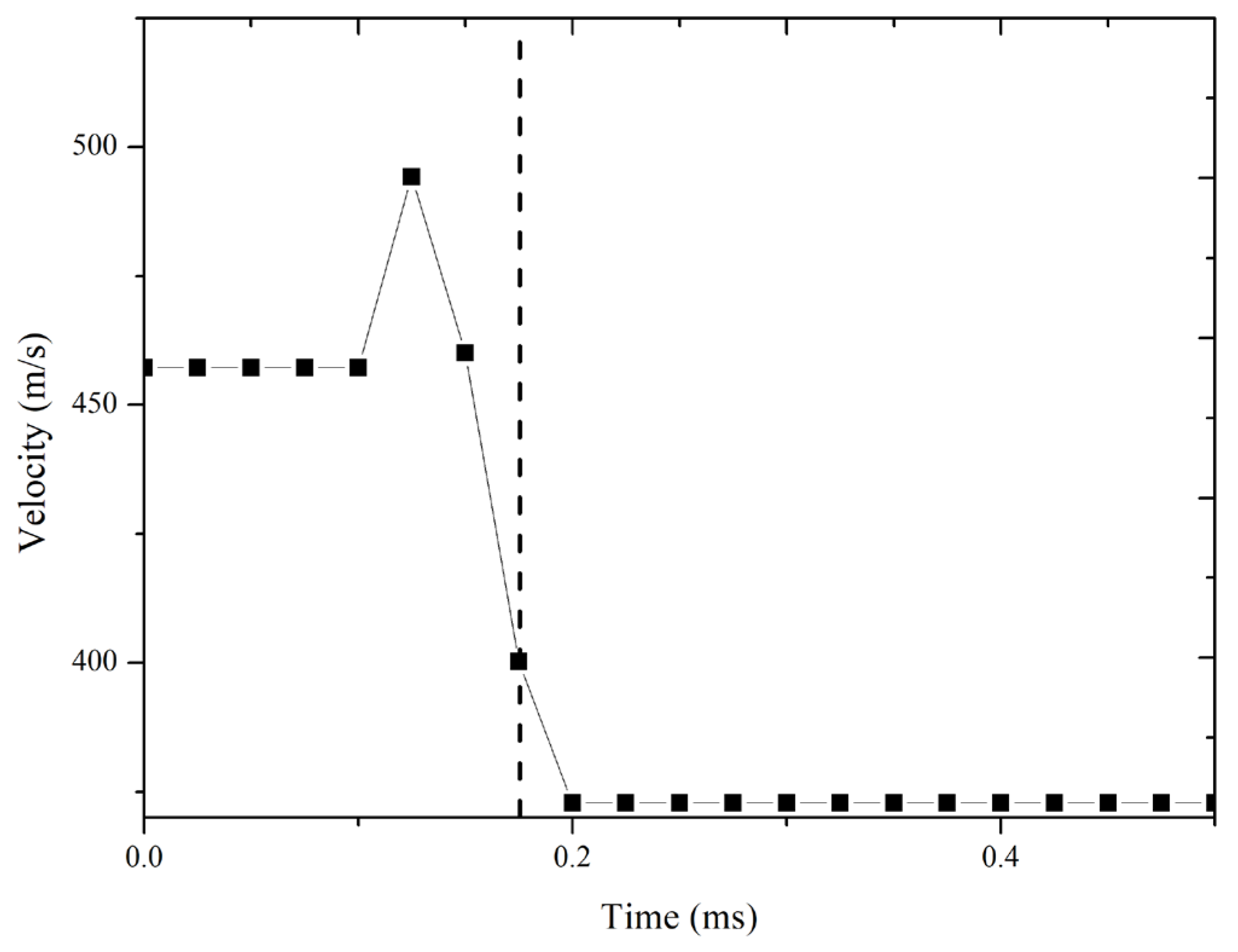
For each time step, the projectile has a specific velocity ($v$) during the sliding in the air. The value of this velocity will affect the amount of projectile kinetical energy ($E_k$) upon the the impact. The simulation result shows the the value of each time step’s velocity evolution and time steps’ graph of AMMMO 2 that is presented in Figure 6 and Figure 7. From the simulation result, velocity after the impact value of 328.74 m/s and 372.85 m/s were obtained, which was later used to calculate the kinetical energy, which is then followed by frangibility calculation. Both graphs show a small velocity increase before a sharp drop because this simulation considers the total velocity from all axes, of which the resultant can cause a small velocity increase and is considered as an error.

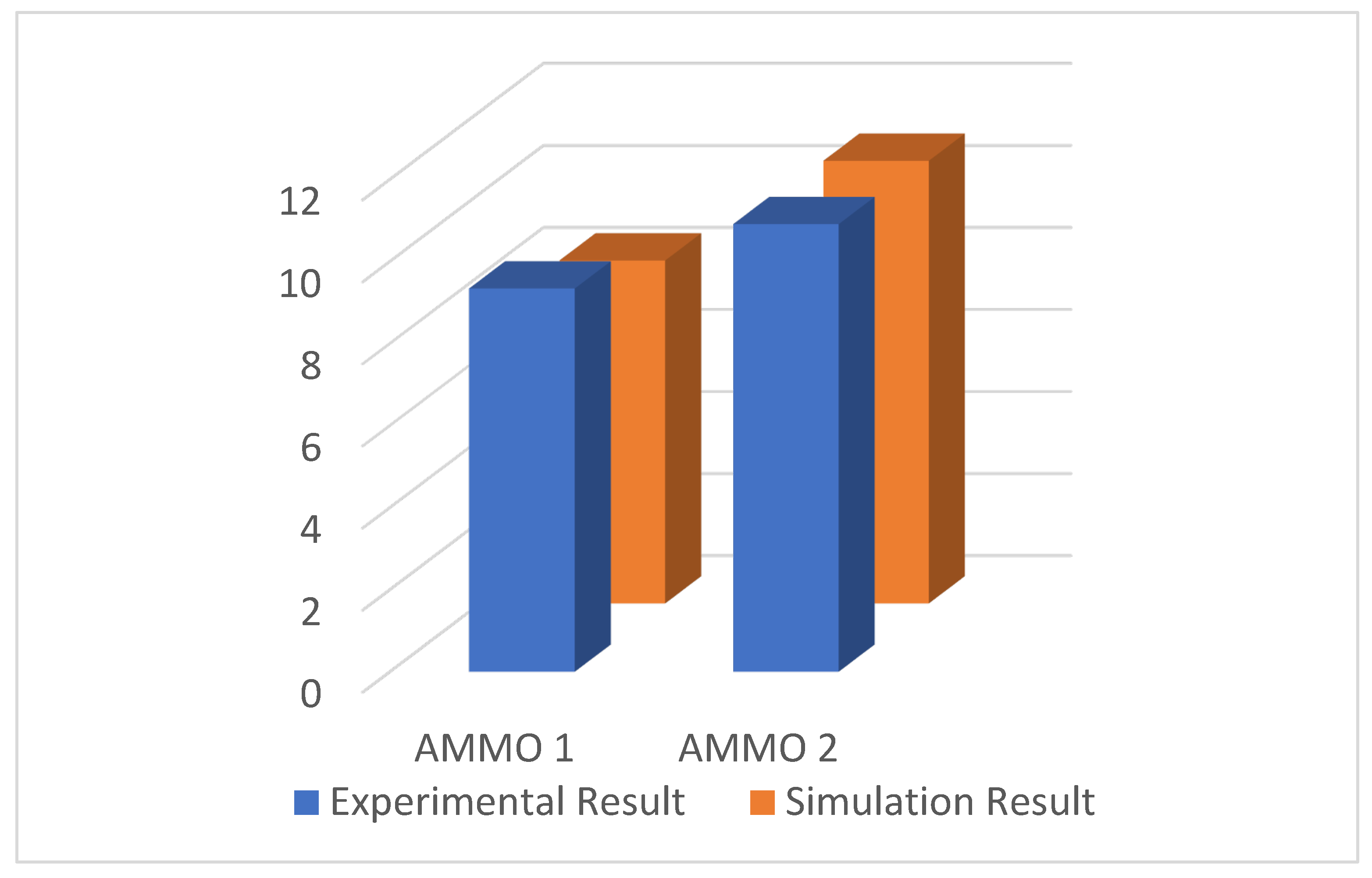
To validate the modelling result, a calculation using the previous equation is conducted. Using the obtained velocity after impact, the kinetical energy can be achieved and then is input to the formulation to define the frangibility factor comparison which can be seen in Figure 8. The calculation result is presented in the

Table 5. Projectile kinetical energy and frangibility factor.

Bullet Designs	Velocity after Impact (m/s)	Kinetical Energy (J)	Kinetical Energy Limit (J)	Frangibility Factor
AMMO 1	383.50	450.04	39.56	8.359
AMMO 2	372.85	363.53	33.67	10.79

.

The obtained frangibility factor data from modelling and calculation will then be compared with the actual frangibility test result. According to previous research, the value of AMMO 1 and AMMO 2 frangibility factors are 9.34 and 10.91, respectively. With these data, the comparison and error from the actual and simulation test results could be calculated, which are presented in the

Table 6. Frangibility factor value comparison.

Projectile Design	Experimental Result	Simulation Result	Error (%)
	FF	FF
AMMO 1	9.34	8359	10.5
AMMO 2	10.91	10.79	1.09

.

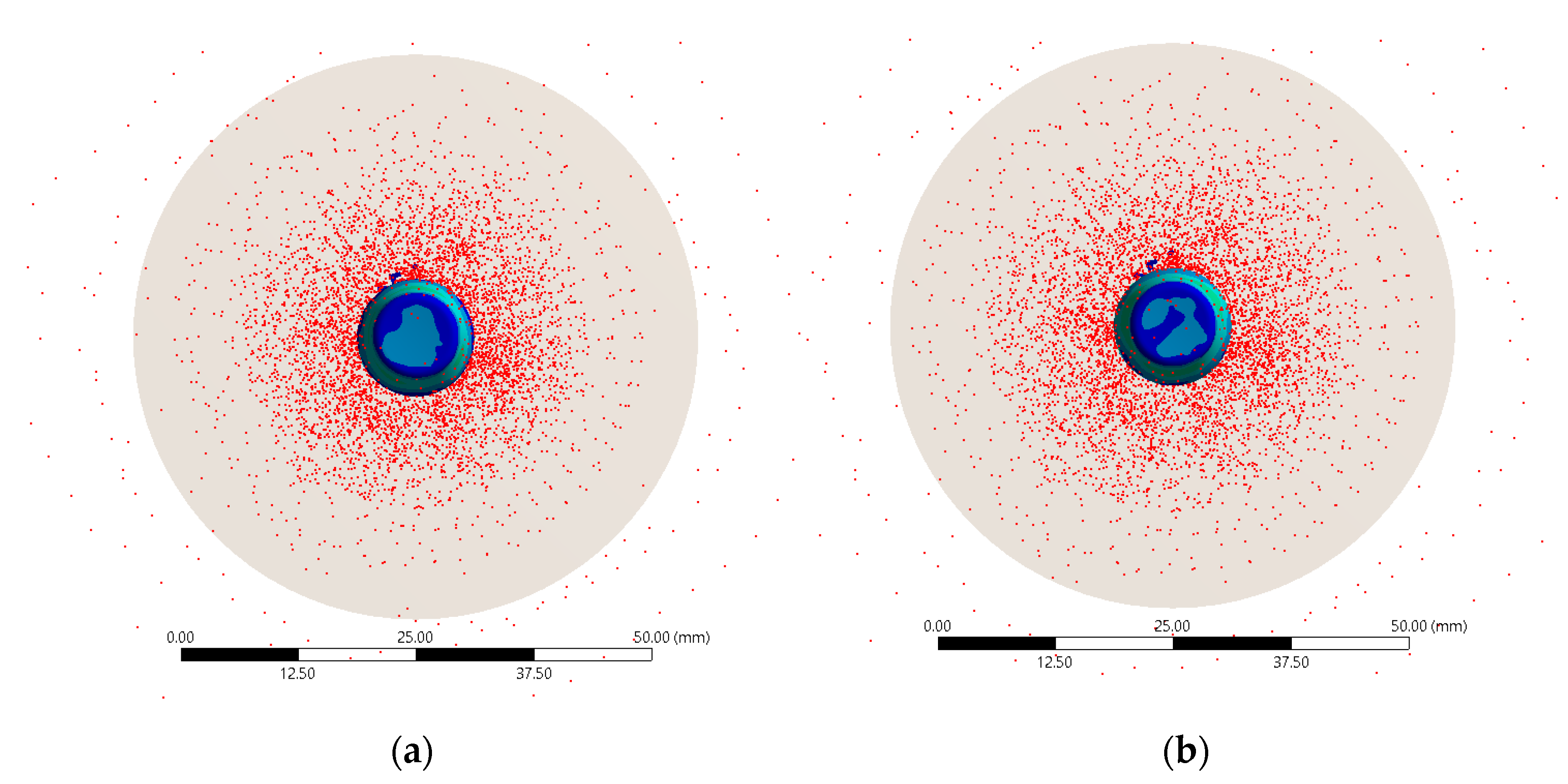
After the modelling process, the projectiles have a certain scattering pattern and distance. This phenomenon is needed to analyze how far the projectile scattered after impact that will affect the frangible bullet safety. It can be seen that AMMO 1 resulted in less projectile fragmentation compared to AMMO 2. However, this method has a limit in determining the particle quantity of the projectile after fragmentation that resulted in a difficulty to quantify the fragmented number of the bullet. The bullet scattering pattern is shown in the Figure 9.

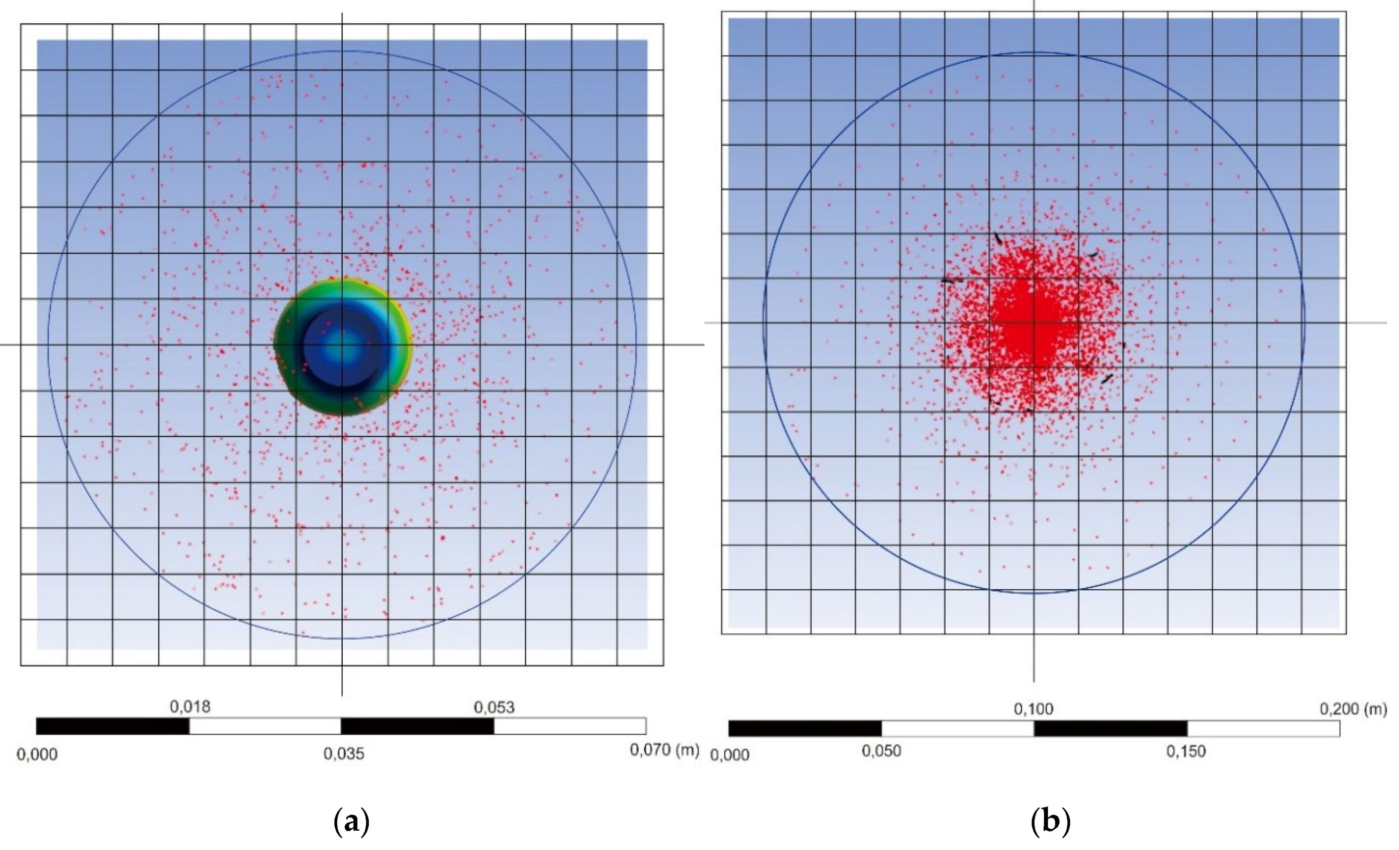
To determine the scattering region of the projectile after impact, the simulation fragmentation results are mapped as Figure 10. Based on this mapping, AMMO 1 in Figure 11a is presented such that the projectile scattering distance which is shown by the ANSYS software is from 0.000 to 0.070 m. Then, the outermost fragment is marked and a straight line is drawn to the center of the impact point which shows 0.0034 m in length. Because the used scale in ANSYS simulation is 1:300, the real distance of the maximum scattering radius for the AMMO 1 is 1.01 m. On the other hand, the scattering region of AMMO 2 shows the measuring length from 0.000 to 0.200 m and the outermost fragment at 0.089 m. These simulation results were then converted to actual scale and the obtained outermost distance of the AMMO 2 was 2.658 m.

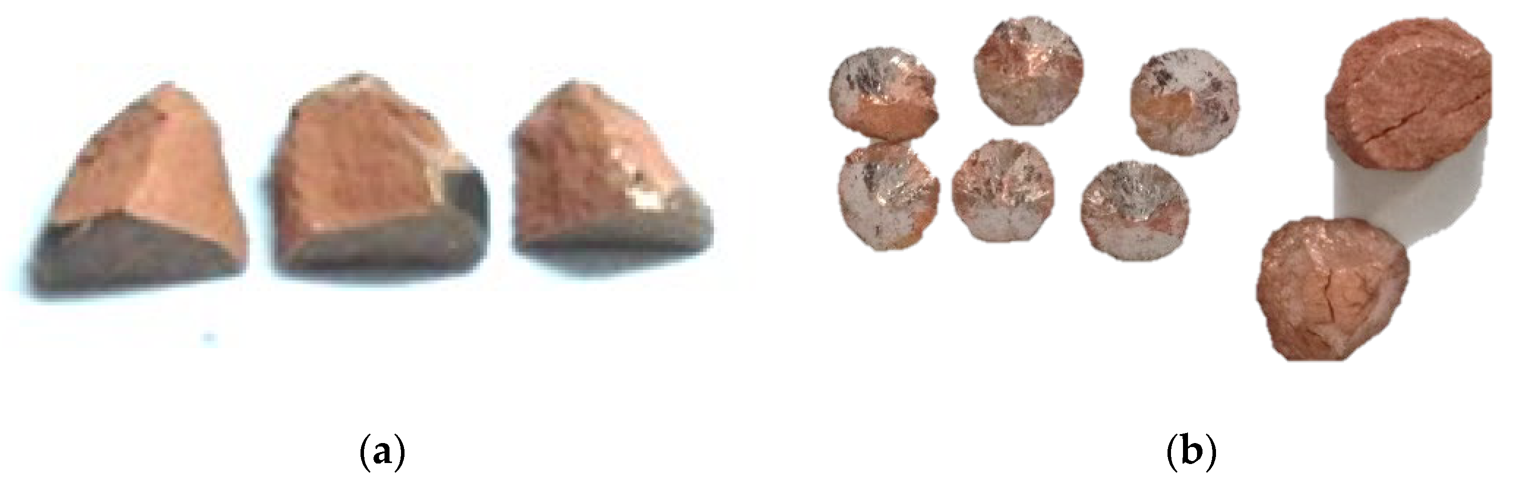
After impact testing, a frangible bullet will experience a disintegration process that results in projectile fragments that vary in size which is shown in Figure 11. The largest fragment formed from the remaining bottom of the fragmented bullet. The fabrication process of this frangible bullet uses powder metallurgy which consists of several main stages. One of the most important stages affecting projectile properties is the compaction process. During the compaction process, which uses single-acting pressing (compaction force from one direction), the bottom of the projectile is the main region with a direct contact and the nearest part to the compaction force, resulting in uneven stress distribution. The bottom part, or the bullet tail, receives more force than the bullet head, which leads to the increasing stress between grains. Moreover, during the impact stage, the bullet head which interacted with the shooting target is the main part which absorbs most of the energy that causes fine fragmentation.

On the contrary, the bullet head received less force, which also reduced the stress applied between grains. High stress between grains will increase the projectile grains’ bounding, which means that high stress results in a stronger property. This phenomenon is the main reason that a fired frangible bullet still not completely be disintegrated, and relatively big fragments do remain. The remaining fragment predominately consists of the bullet tail, while the disintegrated to small fragments are the parts of the bullet head.

Experimentally, Firmansyah et al. conducted ballistic testing using the AMMO 1 design frangible bullet. The ballistic testing was carried out using a plate of 10 mm in thickness, and the fragmented part of the shot bullet was then collected. These collected projectile fragments were then sieved using a vibratory sieve shaker, resulting in different fragment size classifications. On the other hand, Mia et al. also conducted actual ballistic testing using the AMMO 2 design and applied the steel plate thickness as in the previous experiment. These experiment results will then be compared with the simulation result of the remaining bullet fragment. The remaining fragments of the actual experiment are shown in the following figure. For the simulation result, the remaining fragments are shown in Figure 12. It also indicates that the undeformed part of the projectile is larger than the actual bullet fragments.

Principally, the value of the frangibility factor is determined by several primary factors, including projectile characteristics, target mechanical properties, and impact conditions. In this paper, the simulation process mainly focused on the material properties of the frangible bullet, acquired from previous research and frangible bullet standards. For the impact condition, it is assumed to be uniform, so several parameters are adapted with the provided condition and boundary condition of the ANSYS software. The velocity obtained after impact is then used to calculate the kinetical energy, followed by frangibility factor quantification. The first simulation process is of AMMO 1, where the actual experiment was done in the previous research and the obtained kinetical energy value was 450.04 Joule, resulting in a 9.34 frangibility factor number. This actual frangibility calculation was then compared with the simulation process in which the modeling process resulted in an 8.359 frangibility factor number. With the difference between actual and simulation results, the error is acquired at 10.5%. For the AMMO 2, the actual kinetical energy acquired from a real experiment is 363.53 Joule, which resulted in a 10.91 frangibility factor number. Compared with the simulation result, the error obtained was only 1.09%. Overall, the frangibility factor of both modeling processes corresponds with the theory even though the error achieved in AMMO 1 was still relatively high. This error could have appeared due to the complex parameters during the actual experiment that cannot be easily defined by the software. Between the two designs, it is proven that AMMO 2 has better properties due to material characteristics and its design.

For the scattering pattern during fragmentation, the outermost distance of the scattered fragment was 1.01 m for the AMMO 1 and 2.658 m for the AMMO. Visual analysis of the amount of the fragments during disintegration shows that AMMO 2 had more small fragments compared with AMMO 1. This result is in accordance with the theory, which states that a higher frangibility factor will generate more fragments. However, quantitative analysis cannot be done with this method, which resulted in no fragments quantity obtained after the modeling process. In the actual experiment, a projectile is disintegrated into small fragments which have a relatively small mass. The actual ballistic testing result in Figure 11 indicates that the relatively big remaining fragments are mainly composed of the bullet tail. Nevertheless, the simulation result shows different remaining fragments compared to the actual experiment. These differences between the actual experiment and simulation process appeared because the meshing process is limited in the explicit dynamic programs where this meshing process is done in homogenous material, and defects are neglected. During the modeling process, a frangible bullet is considered a perfect homogenous material. Whereas, in the real condition, a frangible bullet has inhomogeneous material distribution and stress, for which the strongest bonds are located in the bullet tail. Parts that have strong grains bonding should have been meshed with a large-sized coarse meshing, and the less grain bonding strength should be meshed with a small-sized fine meshing.

From the actual experiment and simulation process comparison, it can be seen that each method has its own advantages and disadvantages. The main benefit which is offered by real ballistic testing is more precise data acquired and high result accuracy. This high precision is obtained because the complex properties and environmental conditions of the frangible bullet are not neglected. These hard-to-define properties are the real and actual properties, and every bullet has different defects that affect its mechanical characteristics. However, the actual ballistic testing required a longer time and higher cost, so the simulation process became the solution to this issue. A modeling process is considered to be more efficient because the simulation process can be done within a few hours, depending on the meshing size and the time steps. Nevertheless, in this modeling process, several aspects, including material properties and impact conditions, should be validated before executing the process, so the simulation result can approach the actual experimental results. Moreover, the projectile design also has a high impact on the modeling result, so the geometry of the bullet shall be truly considered.

4. Conclusions

In conclusion, the simulation results show that the acquired frangibility factor of each design is 8.359 for AMMO 1 and 10.79 for AMMO 2. With this modeling frangibility factor, the error obtained after comparing with the actual experiment, is 10.5% and 1.09%, respectively. This error can appear because of the complexity of the frangible bullet parameter during the impact phenomenon. Judging from the simulation result, the AMMO 2 projectile design has a better frangibility factor than the other design. According to the scattering pattern analysis, AMMO 2 has more fragments with a longer scattering radius than AMMO 1, which has a value of 1.01 m for AMMO 1 and 2.658 m for AMMO 2, respectively.