1. Introduction
Gene regulation in higher organisms is accomplished at several levels such as transcriptional regulation and post-transcriptional regulation by several cellular processes such as transcription initiation and RNA splicing. In order to better understand these processes, it is desirable to have a good understanding of how transcription factors recognize DNA binding sites and how the spliceosome recognizes RNA splice sites.
Many approaches for the computational recognition of transcription factor binding sites or RNA splice sites rely on statistical models, and two popular models for this task are permuted Markov (PM) models [
1] and permuted variable length Markov (PVLM) models [
2]. The advantage of these models over traditional Markov models such as the position weight matrix model [
3,
4] or the weight array matrix model [
5] is their capability of modeling dependencies among neighboring and non-neighboring positions [
1,
2].
There is evidence that dependencies are not restricted to pairs of positions, which can be modeled by PM models and PVLM models of order one, and that PM models and PVLM models of order two, which are capable of modeling dependencies among triplets of neighboring and non-neighboring positions, outperform PM models and PVLM models of order one [
1,
2]. However, learning optimal PM models and PVLM models of orders one and two is NP-hard, where NP stands for non-deterministic polynomial-time [
6], so heuristics have been used for this problem [
1,
2].
While transcription factor binding sites are typically short and rarely exceed 20 base pairs (bp), it has been shown that the recognition of RNA splice sites can be improved by modeling longer sequences of at least 150 bp [
7]. Hence, it would be desirable to develop exact algorithms capable of learning PM models and PVLM models for RNA splice sites of at least 150 bp in practically acceptable running times.
Learning a pattern from data by a statistical model is often performed in two steps. First, an appropriate model structure reflecting realistic and yet tractable conditional independence assumptions must be learned, and second, appropriate model parameters of the conditional probability distributions must be estimated. Several estimators have been proposed for the second task including the widely used maximum likelihood estimator (MLE). Likewise, several learning principles have been proposed for the first task, and one popular choice is the maximum likelihood principle (MLP).
For PM models and PVLM models of order one, the task of learning the maximum likelihood model results in the traditional Hamiltonian path problem (HPP) or the related traditional traveling salesman problem (TSP). For more powerful PM models and PVLM models of order two, the task of learning the maximum likelihood model results in the quadratic Hamiltonian path problem (QHPP) or the related quadratic traveling salesman problem (QTSP), which are extensions of the traditional linear HPP and TSP, respectively.
Several heuristics for approximately solving QTSPs associated with PM models and PVLM models of order two exist [
8,
9]. However, these heuristics yield quite different solutions with quite different likelihoods, and there are no guarantees about the deviations of the suboptimal solutions from the optimal solution. Moreover, the running times of some of the heuristics are so high that we focus on exact solution methods in this work.
There are several exact algorithms for solving QTSPs [
8–
10], which provide optimal solutions in acceptable running times at least for small instances. Specifically, it has been shown that a branch-and-cut algorithm tailored to the QHPP and the QTSP can solve these problems for random instances up to size 30 in a few hours [
9].
Here, we investigate the performance of this algorithm and two other exact algorithms for learning PM models and PVLM models of order two for RNA splice sites. Specifically, we investigate the performance of these three algorithms for ten datasets of splice acceptor sites and splice donor sites of five different species by measuring their running times for increasing lengths of the studied RNA splice sites until the running times exceed 1.5 × 10⁵ seconds (s), corresponding to approximately two days.
The paper is organized as follows. In Section 2, we summarize the works by Ellrott
et al. [
1] and Zhao
et al. [
2], who introduce PM models and PVLM models, respectively, and who show how to use these models for the recognition of DNA and RNA binding sites. We provide a formal definition of the QTSP in Section 3 and present three exact algorithms for solving this optimization problem in Section 4. We study the running times of these three algorithms for ten datasets of RNA splice sites in Section 5 and conclude the paper in Section 6.
2. Permuted Markov Models and Permuted Variable Length Markov Models
Nucleotide sequences of transcription factor binding sites and splice sites are not statistically independent, and one of the challenges of bioinformatics is to devise statistical models that can capture dependencies among neighboring and non-neighboring positions that are omnipresent in both transcription factor binding sites and splice sites. Two powerful models for the recognition of transcription factor binding sites and splice sites that are capable of capturing such dependencies are PM models and PVLM models proposed by Ellrott
et al. [
1] and Zhao
et al. [
2]. The key idea of both models is to allow a permutation of the ordering of nucleotides of a binding site and then to define a Markov model or a variable length Markov model over that permuted binding site.
Consider a dataset D of sequences x of length L over a discrete, finite alphabet Σ, and consider a PM model or PVLM model for modeling these sequences. The central structure of these models is a permutation π of positions 1,…, L. We denote the predecessors of πℓ in permutation π by pre(π, ℓ). Specifically, pre(π, ℓ) returns πℓ−1 (if ℓ > 1) for PM models and PVLM models of order one, (πℓ−1, πℓ−2) (if ℓ > 2) for PM models and PVLM models of order two and, in general, (πℓ−1,…, πℓ−d) (if ℓ > d) for PM models and PVLM models of order d, while pre(π, ℓ) returns (π1,…, πℓ−1) for ℓ ≤ d.
Given a permutation
π, the log-likelihood of a PM model can then be written as a sum of
L position-specific terms, where the
ℓ-th term depends only on position
πℓ and its predecessor pre(
π, ℓ). Specifically, the log-likelihood of a single sequence
x given permutation
π can be written as:
and the likelihood of an independent and identically distributed dataset
D given permutation
π can be written as:
Using maximum likelihood estimators for the model parameters, the conditional probabilities on the right-hand side can be replaced by ratios of absolute frequencies as follows. For a dataset
D of
N sequences
x, we denote the absolute frequency of observing oligonucleotide
y at position
i by:
the absolute frequency of observing oligonucleotide
y at position
i and nucleotide
z at position
j by:
the relative frequency of observing oligonucleotide
y at position
i by:
and the conditional relative frequency of observing nucleotide
z at position
j given oligonucleotide
y at position
i by:
Based on that, the maximum log-likelihood of dataset
D given permutation
π can now be rewritten as:
where Σ
|pre(π,ℓ)| denotes the set of sequences over Σ of length |pre(
π, l)|, and
denotes the frequency estimator of the conditional Shannon entropy of nucleotide
at position
πℓ given oligonucleotide
Xpre(π,ℓ) at position pre(
π, ℓ) in units of nats. Hence,
Equation (1) states that the maximum log-likelihood of dataset
D given permutation
π is given by a sum of
L position-specific terms, where the
ℓ-th term depends only on positions pre(
π, ℓ) and
πℓ.
Computing the maximum log-likelihood log
P (
D|
π) of a dataset
D given a permutation
π is straightforward, but finding an optimal permutation
π that maximizes the log-likelihood log
P (
D|
π) over all
L! permutations
π is non-trivial. Mathematically, this optimization problem can be stated as:
and we present the connection to the QTSP in the following section.
3. Quadratic Traveling Salesman Problem
In this section, we formally introduce the QHPP and the QTSP. Given a complete directed graph G = (V, A) with a set of nodes V = {1,…, L}, L ≥ 3, a set of arcs A = V(2) := {(i, j): i, j ∈ V, i ≠ j}, and an associated set of two-arcs V(3) := {(i, j, k): i, j, k ∈ V, |{i, j, k}| = 3} (a two-arc (i, j, k) is an ordered sequence of pairwise distinct nodes i, j, k), a sequence of nodes (v1, v2,…, vk) is called a path if all vi ∈ V, i ∈ {1,…, k}, are pairwise distinct. Similarly, a sequence of nodes (v1, v2,…, vk, v1) is called a cycle in G if all vi ∈ V, i ∈ {1,…, k}, are pairwise distinct. A path (v1, v2,…, vk) or a cycle (v1, v2,…, vk, v1) in G is called Hamiltonian if k = L, and a Hamiltonian cycle is also called a tour.
For given arc weights
cl :
V(2) → ℝ and two-arc weights
cq :
V(3)→ ℝ, the total costs of a path
Q = (
v1,…,
vk) w. r. t. to
cl or
cq are:
respectively.
Similarly, the total costs of the corresponding cycle
C = (
v1,…,
vk, v1) w. r. t. to
cl or
cq are:
respectively.
With these definitions, the weighted Hamiltonian path problem (HPP) is to:
and the weighted quadratic Hamiltonian path problem (QHPP) is to:
The TSP that asks for a cost-minimal tour w. r. t.
cl can be formulated in a similar way by replacing the Hamiltonian path
Q with a Hamiltonian cycle
C, and the QTSP that asks for a cost-minimal tour w. r. t.
cq can be formulated analogously by replacing the Hamiltonian path
Q with a Hamiltonian cycle
C. That is, the TSP is to:
and the QTSP is to:
i.e., the QTSP differs from the TSP only in that the cost of a tour depends on each triple, and not only on each pair, of nodes that are traversed in succession in the tour.
An HPP can be easily transformed into a TSP on a larger graph by inserting an additional artificial node and by setting the costs of the additional arcs appropriately. Likewise, a QHPP can be easily transformed into a QTSP on a larger graph by inserting an additional artificial node and by setting the costs of the additional two-arcs appropriately.
For modeling the QHPP, we consider a QTSP on the complete graph
with set of nodes
, where the artificial node 0 is used to model the first summands in
Equation (1) and to allow for a complete definition of
and
. Specifically, we set:
for arcs
and two-arcs
, respectively.
Based on these definitions, an optimal permutation
π of problem (
2) can be obtained by solving a QTSP.
4. Exact Algorithms
In this section, we describe three exact algorithms for solving the NP-hard QTSP. First, we present a simple algorithm based on dynamic programming in Section 4.1. Second, we present a branch-and-bound algorithm based on some combinatorial lower bounds in Section 4.2. Finally, we present a branch-and-cut algorithm based on integer programming in Section 4.3.
4.1. Dynamic Programming Algorithm
The following dynamic programming (DP) algorithm for solving the QTSP is an extended version of a DP algorithm for solving the TSP [
11]. For the sake of simplicity, we solve the QHPP on the graph
with the additional node 0 as the fixed first node of the path, so we consider only the nodes in
V in the remainder of this subsection.
For a subset
W ⊆ V and two nodes
j, k ∈ W and
j ≠
k, we compute the optimal costs
BW,j,k for any path visiting all nodes of
W, with
j and
k being the last two nodes in this order by the recursion:
We perform this recursion bottom-up for all subsets W ⊆ V, i.e., we start with all subsets of size two, then continue with all subsets of size three, etc., which ensures that the partial solutions needed in the recursion are already computed.
The minimal costs for a quadratic Hamiltonian path can finally be determined by:
and the corresponding path can be derived by backtracking.
4.2. Branch-and-Bound Algorithm
The branch-and-bound (BnB) algorithm was first described by Land and Doig in 1960 [
12]. The idea for solving minimization problems with discrete decisions, e.g., whether an arc is contained in a tour or not, is the following. Fixing parts of the solution and creating several subproblems (branching), we compute local lower bounds for each of the subproblems that are compared to the currently best solution. If the lower bound of one of the subproblems is larger than the value of the currently best solution, we can delete this subproblem, because it cannot lead to an optimal solution. Furthermore, we update the best solution if we find a better solution during the subproblem calculations. The hope is that, instead of testing all possible cases, the solution space can be reduced significantly by the lower bound calculations.
The BnB algorithm for the QTSP traverses all possible tours in the worst case. In the branching part, we create subproblems by fixing subpaths. Each time we consider a new subpath, we compute a lower bound for a QTSP solution containing this subpath. Here, we use as a lower bound the solution of some cycle cover problem (CCP), which asks for an arc-cost minimal set of cycles
K = {
C1,…,
Ck} such that each node is contained in exactly one cycle. As the objective function for the CCP, we use the coefficients:
for the arcs (
u, v)
∈ V(2). With this definition of the arc costs, we ensure that the optimal value of the CCP is a lower bound of the optimal value of the associated QTSP, because for each two-arc (
u, v, w′)
∈ V(3) contained in an optimal QTSP solution, we only count the costs
cq((
u, v, w)) with
, associated with the arc (
u, v) in the CCP. The advantage of the described transformation to a CCP is that the CCP can be solved in polynomial time by the Hungarian method [
13], which allows us to derive lower bounds in polynomial time. We start all tours with a fixed node
v1, which is chosen in such a way that the sum over all values
cq((
v1,
u, w)) with (
v1,
u, w)
∈ V(3) is maximal. The motivation for this choice is that we hope that the lower bounds in the first steps are rather large, allowing us to prune several subproblems close to the beginning.
4.3. Branch-and-Cut Algorithm
Branch-and-cut (BnC) algorithms have been very successful for solving the TSP [
10,
14–
16]. Given an integer programming (IP) formulation, we consider a relaxation of the problem by dropping the integrality constraints of the variables and possibly some of the constraints. As we will see below, the standard formulations for the TSP and the QTSP contain an exponential number of constraints. Hence, it is practically impossible to add all constraints to the model at once. The BnC approach combines linear programming for solving the relaxation with a so-called cutting-plane approach, which starts with a restricted number of constraints and adds them successively during the solution process if they are violated. In order to improve the formulation, one usually separates further cutting planes that tighten the current relaxation to obtain even stronger bounds. Furthermore, the BnC approach combines the cutting plane approach based on linear programming with a BnB approach.
The standard IP formulation for the TSP of Dantzig
et al. [
14] uses binary arc variables
ra ∈ {0, 1},
a ∈ A, with the interpretation
ra = 1 if and only if the arc
a is contained in the tour and zero otherwise. It reads:
The degree constraints (
3) ensure that each node is entered and left exactly once by the tour. Cycles of a length less than
L are forbidden by the well-known subtour elimination constraints (SEC) (
4). Finally, condition (
5) ensures the integrality of the variables.
Concerning the QTSP, each two-arc (
u, v, w)
∈ V(3) is contained in a tour if and only if the two associated arcs (
u, v) and (
v, w) are both contained in the tour. Hence, we can formulate the QTSP as an IP with quadratic objective function:
Linearizing this objective function by replacing each product
r(u,v) · r(v,w) with a new binary variable
t(u,v,w) ∈ {0, 1} for each two-arc (
u, v, w)
∈ V(3), we derive the following linear IP formulation for the QTSP:
Constraints (
6) couple the arc variables and the two-arc variables. If an arc (
u, v)
∈ A is contained in the tour, there must be a node
w ∈ V so that the path (
u, v, w) is part of the tour and a node
w′ ∈ V so that the path (
w′, u, v) is part of the tour.
In the BnC approach, we use constraints (
3) and (
6),
ra ∈ [0, 1],
a ∈ A, and
t(u,v,w) ∈ [0, 1], (
u, v, w)
∈ V(3), as a basic relaxation. In order to obtain an exact algorithm for the QTSP, it is sufficient to separate the standard subtour elimination constraints (
4). However, in order to speed up the algorithm, we add further cutting planes known to be valid for the QTSP.
Lemma 1: See [
17]:
The triangle inequalities of Type I:are valid for the QTSP for all u, v, w ∈ V, |{
u, v, w}| = 3,
L ≥ 4.
The triangle inequalities of Type II:are valid for the QTSP for all S ⊆ V, |
S| = 3.
The strengthened subtour elimination constraints:are valid for the QTSP for all.
The triangle inequalities (
8) forbid cycles of length three. If
L ≥ 4, at most one of the two two-arcs (
u, v, w) and (
w, u, v) can be contained in a tour. However, if one of these two two-arcs is contained in the tour, then also arc (
u, v) is contained in the tour. The validity of inequalities (
9) follows from the fact that at most two of the corresponding arcs can be contained in a tour, but if two arcs are contained in the tour, also one of the two-arcs is contained in the tour. Inequalities (
10) are a strengthened version of inequalities (
4), where we do not only count the direct connections between two nodes
u, v ∈ S, u ≠
v, but also the connections with one node between them.
Inequalities (
8)–(
10) are even facet-defining for the polytope associated with the QTSP [
17] if
L is sufficiently large. Considering the separation problems for the three inequality classes, a violated inequality of the first two classes can be determined in polynomial time, because there are only
such inequalities. A maximally-violated subtour elimination constraint (
4) can be determined in polynomial time by minimum-cut calculation [
18], because constraints (
4) are equivalent to
,
,
. In contrast to this, it has been shown in [
17] that determining a maximally-violated constraint of type (
10) is NP-hard. For this reason, we explicitly separate all inequalities (
10) for sets
S ⊂ V with |
S| = 2 and use a heuristic approach for separating inequalities (
10) in general in our experiments.
5. Experimental Study
In this section, we study the running times of the three algorithms presented in Section 4 on ten datasets of splice acceptor sites and splice donor sites from five different species of lengths up to 200 bp. We implemented all algorithms in C++ and Java using the following subroutines. For the BnB algorithm, we used the CCP solver implemented by Jonker and Volgenant [
19], which is based on the Hungarian method. For the BnC algorithm, we used the BnC solver Gurobi 5.6.3 [
20], which we extended by problem-specific cutting planes. For the separation of the subtour elimination constraints (
4), we used the software package Lemon [
21]. If a cut of value less than one is found, we separate constraints (
10) instead of constraints (
4). Furthermore, we built separators for inequalities (
8) and (
9) and for inequalities (
10) with sets
S ⊂ V, |
S| = 2, which are based on complete enumeration. We carried out all experiments on a PC with an Intel ® Core
™ i7 CPU 920 with 2.67 GHz and 12 GB RAM.
From each of the ten datasets, we extract all splice sites, truncate the surrounding sequences to length
L symmetrically around the splice sites, and apply each of the three algorithms presented in Section 4 to each of these ten datasets containing subsequences of length
L. We stop each algorithm if its running time exceeds 1.5×10
5 s, corresponding to approximately two days, and record its running time otherwise. Finally, we plot the running times as a function of the sequence length
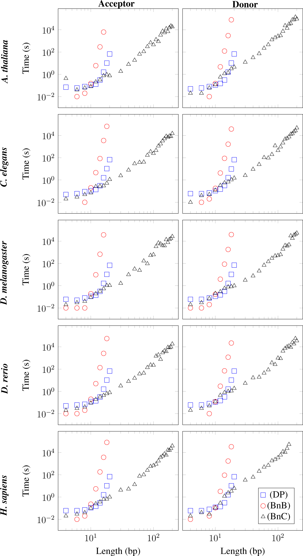
L ranging from 4 bp to 200 bp for each of the three algorithms and each of the ten datasets in
Figure 1.
Figure 1 shows that the running time of the DP algorithm increases super-exponentially with
L, as expected theoretically. For the ten datasets studied, the DP algorithm is capable of solving the QTSP for
L = 20 bp in approximately 70 s, whereas it is not capable of solving the QTSP for
L ≥ 30 bp in less than 1.5 × 10
5 s.
Figure 1 further shows that the BnB algorithm is faster than the DP algorithm for short sequences of
L ≤ 10 bp, but that its running time increases dramatically with growing
L so that the BnB algorithm is not capable of solving the QTSP for
L = 20 bp in less than 1.5 × 10
5 s for any of the ten datasets studied.
Finally, we observe in
Figure 1 that the running time of the BnC algorithm is comparable to that of the DP algorithm for short sequences of
L ≤ 10 bp, but that its running time increases substantially more slowly with
L than that of the DP algorithm for
L ≥ 10 bp. Surprisingly, the BnC algorithm is capable of solving the QTSP for
L = 200 bp in less than 1.5 × 10
5 s for nine of the ten datasets studied. The average running times for
L = 50 bp, 100 bp, 150 bp, and 200 bp can be found in
Table 1.
The running times of the BnC algorithm are significantly shorter than those of the other two algorithms. Even if we assume an only exponential increase of the running time of the DP algorithm with L and a crude theoretical lower bound of 2L, we obtain a running time for the DP algorithm of more than 1056 s for L = 200 bp, stating that the BnC algorithm is at least 50 orders of magnitude faster than the currently fastest algorithm for solving the QTSP for splice donor sites and splice acceptor sites of L = 200 bp.
The surprisingly small running times of the BnC algorithm can be explained as follows. There are usually less than one hundred nodes in the BnC tree. Hence, for the ten datasets studied, the cutting planes introduced in Section 4 are very effective and much better than for the random instances studied in [
9].
6. Conclusions
The computational recognition of RNA splice sites is an important task in bioinformatics, and two popular models for this task are permuted Markov models and permuted variable length Markov models. However, learning permuted Markov models and permuted variable length Markov models is NP-hard and, thus, a challenging problem for the recognition of RNA splice sites, because it could be shown that sequences of at least 150 bp surrounding the splice sites should be taken into account for a reliable recognition of RNA splice sites. Hence, learning permuted Markov models and permuted variable length Markov models could be performed only heuristically in the past.
Learning optimal permuted Markov models and optimal permuted variable length Markov models of order two, however, is equivalent to the quadratic traveling salesman problem (QTSP), and a recently-developed BnC algorithm based on integer programming has been capable of solving randomly-generated instances up to instance sizes of 30. Hence, we have investigated in this paper the capability of this algorithm and two additional algorithms for learning permuted Markov models and permuted variable length Markov models, a DP algorithm and a BnB algorithm, for ten datasets of splice acceptor sites and splice donor sites.
We have found that the BnC algorithm based on integer programming is by orders of magnitude more effective than the DP algorithm and the BnB algorithm. Specifically, we have found that the BnC algorithm is capable of learning permuted Markov models and permuted variable length Markov models from splice sites of lengths up to 200 bp in less than two days.


