Assessment of Density-Functional Tight-Binding Ionization Potentials and Electron Affinities of Molecules of Interest for Organic Solar Cells Against First-Principles GW Calculations

Abstract

Ionization potentials (IPs) and electron affinities (EAs) are important quantities input into most models for calculating the open-circuit voltage ($V_{oc}$) of organic solar cells. We assess the semi-empirical density-functional tight-binding (DFTB) method with the third-order self-consistent charge (SCC) correction and the 3ob parameter set (the third-order DFTB (DFTB3) organic and biochemistry parameter set) against experiments (for smaller molecules) and against first-principles $GW$ (Green’s function, G, times the screened potential, W) calculations (for larger molecules of interest in organic electronics) for the calculation of IPs and EAs. Since $GW$ calculations are relatively new for molecules of this size, we have also taken care to validate these calculations against experiments. As expected, DFTB is found to behave very much like density-functional theory (DFT), but with some loss of accuracy in predicting IPs and EAs. For small molecules, the best results were found with ΔSCF (Δ self-consistent field) SCC-DFTB calculations for first IPs (good to ± 0.649 eV). When considering several IPs of the same molecule, it is convenient to use the negative of the orbital energies (which we refer to as Koopmans’ theorem (KT) IPs) as an indication of trends. Linear regression analysis shows that KT SCC-DFTB IPs are nearly as accurate as ΔSCF SCC-DFTB eigenvalues (± 0.852 eV for first IPs, but ± 0.706 eV for all of the IPs considered here) for small molecules. For larger molecules, SCC-DFTB was also the ideal choice with IP/EA errors of ± 0.489/0.740 eV from ΔSCF calculations and of ± 0.326/0.458 eV from (KT) orbital energies. Interestingly, the linear least squares fit for the KT IPs of the larger molecules also proves to have good predictive value for the lower energy KT IPs of smaller molecules, with significant deviations appearing only for IPs of 15–20 eV or larger. We believe that this quantitative analysis of errors in SCC-DFTB IPs and EAs may be of interest to other researchers interested in DFTB investigation of large and complex problems, such as those encountered in organic electronics.

1. Introduction

Organic electronics is a rapidly-growing alternative to silicon-based electronics. In contrast to the latter, which is well enough understood [1], that fabless manufacturing may be used for circuit design using modeling software, such as SPICE [2], and then be outsourced to a semiconductor foundry for actual fabrication, organic electronics is a rapidly growing, but much less well understood [3,4,5,6,7,8] technology. One example is organic solar cells [9,10,11,12], which offer the advantage of being relatively inexpensive to manufacture, flexible and printable. The problem then is to be able to understand such devices well enough to be able to optimize and ultimately to engineer devices with them. This implies modeling, and modeling of organic solar cells almost always requires ionization potentials (IPs) and electron affinities (EAs) as input. However, the size of the molecules (or clusters of molecules) used in modeling organic solar cells rapidly makes first-principles calculations prohibitive, if not impossible. The semi-empirical density-functional tight-binding (DFTB) method is highly attractive for overcoming size and complexity modeling constraints, but it needs to be carefully assessed to determine the expected accuracy. In this paper, we complement previous efforts [13,14] ([14] concerns implementing range-separated hybrids in DFTB [15,16]) by assessing DFTB against accurate first-principles $GW$ (Green’s function, G, times the screened potential, W) calculations [17,18,19] for the calculation of the IPs and EAs of medium-sized molecules.

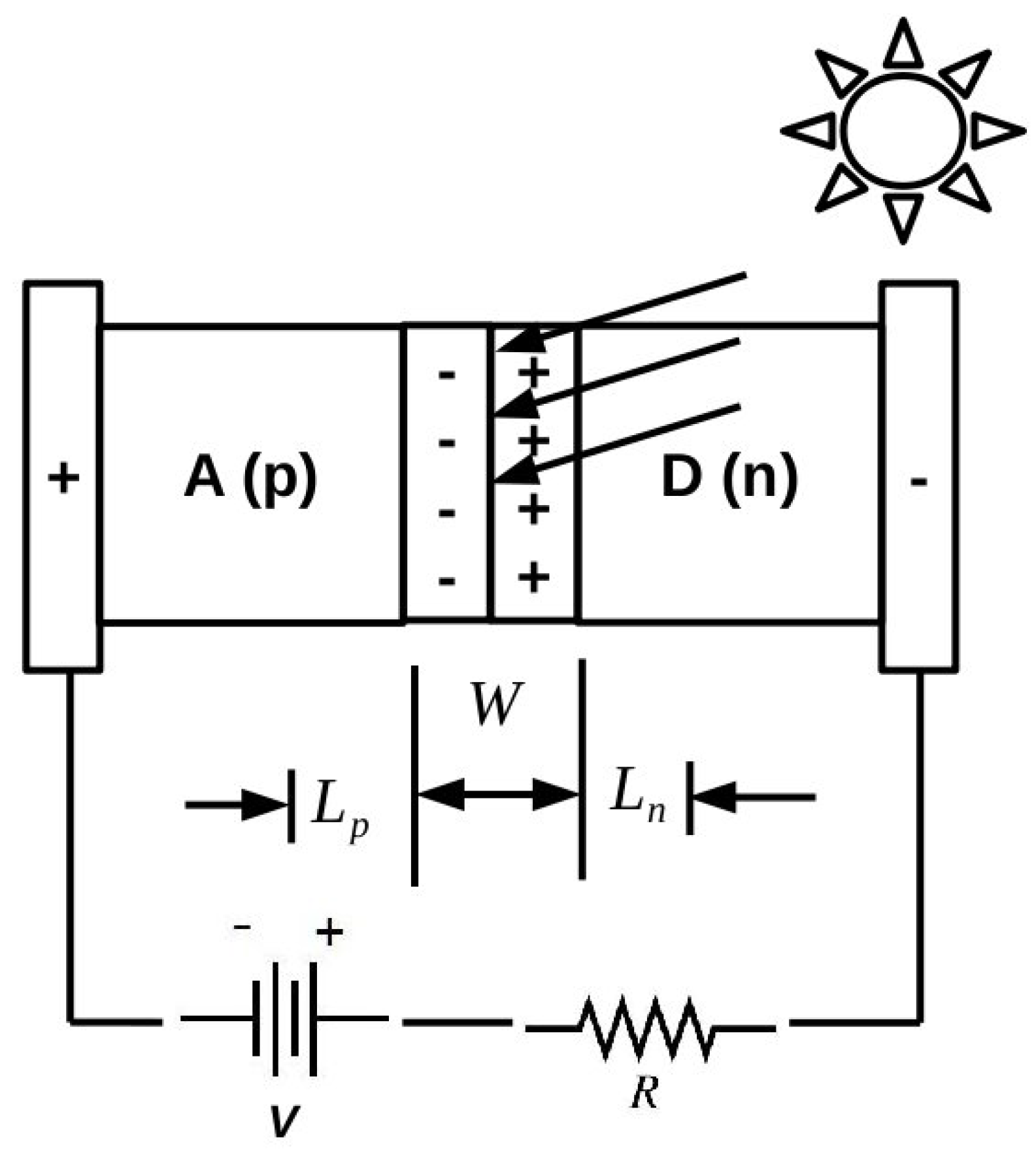
Our particular interest is in modeling organic solar cells for which phenomenological models are reviewed in the Appendix. Ideally, we would like to be able to extract parameters for these models from atomistic modeling. Given the size and complexity of minimum-sized cluster models or unit cells of periodic models for a reasonable description of organic solar cells, it is clear that we need a highly efficient method. This is especially clear for such things as charge diffusion lengths and the size of depletion zones. However, this is also true for the seemingly relatively straightforward calculation of IPs and EAs. Figure 1 gives minimum size examples of some typical molecules that are used in organic electronics. While some are “medium-sized” molecules, which come within the range of ab initio calculations, many of the examples shown are just oligomers intended to represent the much longer polymers used in real organic solar cells. To make matters worse, charge transfer excitons are often present, which are delocalized over several “medium-sized” molecules, so that it is necessary to use clusters of molecules to have a physically-reasonable model. All of these reasons encourage us to look for an efficient and hopefully reasonably accurate semi-empirical approach. An appealing approach that may meet our needs is the density-functional tight-binding (DFTB) approach, which will be briefly reviewed in the next section. To our knowledge, there is only one previous application of DFTB to organic solar cells [13]. That study focused on the problem of calculating charge transfer energies and made a comparison against experimental values.

Figure 1. Eight typical molecules that are often used as acceptors or donors in organic electronics.

Figure 1. Eight typical molecules that are often used as acceptors or donors in organic electronics.

We have chosen a different approach to assessing the accuracy of DFTB here by choosing to compare DFTB IPs and EAs against first-principles $GW$ values. The advantage of this approach is that experimental IPs and EAs for large molecules are often extracted from condensed phase (bulk, thin film or solution) measurements, introducing uncertainties when it comes to trying to extract molecular values. We will show that our $GW$ calculations do indeed give good IPs when compared to experimental IPs for medium-sized molecules, and we will then assume that this is also true for the other medium-sized molecules, where molecular IPs are not available and also for EAs. Taking the $GW$ values as the “true values”, we then calculate error bars on the DFTB estimate of the $GW$ values.

The rest of this paper is organized as follows: the next section gives a brief review of the basic electronic structure methods used in this paper. Section 3 provides computational details. Section 4 goes on to describe and apply our analytical procedure for assessing the quality of DFTB IPs and EAs for the case of small molecules where good and theoretically well-understood experimental data are available. This gives us a useful first indication of how DFTB might work for the case that really interests us, namely for larger molecules of interest in organic electronics. Section 5 then extends our analysis to a set of medium-sized molecules typical of organic electronics. The assessment is complicated by the dearth of theoretically well-understood experimental data. We show that this dearth of experimental data may be compensated by high-quality $GW$ calculations, which agree well with available experimental data, and best when for gas phase data, where the comparison is cleanest. We therefore use the $GW$ results as our benchmark for evaluating DFTB IPs and EAs for medium-sized molecules. Section 6 provides a concluding discussion.

2. Theoretical Methods

While the Hartree–Fock (HF) approximation and density-functional theory (DFT) are now so familiar that they hardly seem worth discussing, this is less the case for $GW$ Green’s function calculations and for the DFTB semiempirical approximation to DFT (HF is treated in most text books on quantum chemistry, such as [20], while DFT is treated in many recent text books; nevertheless more detailed information regarding DFT may be found in [21,22,23,24,25]). These latter approaches will be briefly described in this section, with emphasis on calculating IPs and EAs. Unless otherwise specified, we will use Hartree atomic units ($\hslash =m_e=e=1$). We will also use a reduced notation where $q=({\mathbf{r}}_q,{\sigma }_q)$ represents the space and spin coordinates of particle q while $\mathbf{q}=(q,t_q)$ (bold face) is enriched to include time.

All approaches involve a molecular orbital (MO) equation,

$$\widehat{f}(1;{ϵ}_s){\psi }_s\left(1\right)={ϵ}_s{\psi }_s\left(1\right)$$

(1)

The MO Hamiltonian has the form,

$$\widehat{f}(1;\omega )={\widehat{h}}_H\left(1\right)+{\widehat{\Sigma }}_{xc}(1,\omega )$$

(2)

where ${\widehat{h}}_H$ is the Hartree Hamiltonian. The frequency-dependence of the self-energy belongs to the $GW$ method and does not apply for the HF approximation nor for Kohn–Sham DFT. The exchange-correlation (xc) “self-energy”, ${\widehat{\Sigma }}_{xc}(1;\omega )$, is just the exchange integral operator [$-\widehat{K}\left(1\right)$] in HF and the functional derivative $v_{xc}\left(1\right)=\delta E_{xc}/\delta \rho \left(1\right)$ in pure DFT (we use ρ for the density). The MO equation is obtained in both cases from the variational minimization of the corresponding energy expressions. It is now also common practice to mix HF and pure DFT to make hybrid functionals, such as the popular B3LYP functional.

One way to calculate the (first) IP, I, and (first) EA, A, in DFT is to carry out self-consistent field calculations of the total energies for the N-electron system, the $(N-1)$-electron system and the $(N+1)$-electron system. The ΔSCF (Δ self-consistent field) IPs and EAs are then given respectively by,

$$\begin{array}{c}\hfill \begin{array}{ccc}\hfill I_S& =\hfill & E_S^{(N-1)}-E_0^{\left(N\right)}\\ \hfill A_S& =\hfill & E_0^{\left(N\right)}-E_S^{(N+1)}\end{array}\end{array}$$

(3)

where $E_0^{\left(N\right)}$ is the energy of the ground state of the N-electron molecule, $E_S^{(N-1)}$ is the energy of the same system with one electron removed in its S-th electronic state and $E_S^{(N+1)}$ is the energy of the same system, but with one more electron in its S-th excited state. Note that the concepts of IP and EA have thus been generalized beyond the usual definition where $S=0$ (ground state). Together, the IPs and EAs form a (generalized) band spectrum. Note also that S is a state label, as opposed to an MO label, which would have been a small s. In the quasiparticle part of the band spectrum, each principle IP or EA corresponds to removing or adding an electron to an orbital s. In this case, S may be identified with s. The ΔSCF IPs and EAs may be estimated using Slater’s transition orbital method, whereby the ΔSCF IP or EA is given by minus the orbital energy recalculated with half an electron removed from or added to the orbital. The ΔSCF method works for small molecules, but must inevitably fail for pure DFT (where the density functional depends only on the density as in the local density approximation (LDA) or generalized gradient approximations (GGAs)) in the limit of a large system with delocalized hole and electron states, because the change in the charge density is then insignificant [26]. Furthermore, the ΔSCF method is known to fail to give good IPs and EAs in the HF approximation, because it includes only relaxation effects and not correlation effects, which are known to partially cancel each other for outer valence ionization. In this case, it is better to use Koopmans’ theorem IPs and EAs, which are just the negative of the orbital energies. Such IPs and EAs are still approximate.

2.1. Green’s Function Methods

Green’s function methods may be thought of as adding terms to the xc self-energy, so that Koopmans’ theorem IPs and EAs become exact. That is, minus the energies of the occupied orbitals are the vertical IPs, and minus the unoccupied orbital energies are the vertical EAs. More exactly, the MO equation has two types of solutions, namely the IP solutions and the EA solutions. For the IP solutions,

$$\begin{array}{c}\hfill \begin{array}{cc}\hfill {ϵ}_S& =E_0^{\left(N\right)}-E_S^{(N-1)}\hfill \\ \hfill {\psi }_S\left(1\right)& =\langle {\Psi }_S^{(N-1)}|\widehat{\psi }\left(1\right)|{\Psi }_0^{\left(N\right)}\rangle \hfill \\ & =\sqrt{N}\int {\left({\Psi }_S^{(N-1)}(2,3,\cdots ,N)\right)}^{*}\hfill \\ & \times {\Psi }_0^{\left(N\right)}(1,2,3,\cdots ,N)d2d3\cdots dN\hfill \end{array}\end{array}$$

(4)

while for the EA solutions,

$$\begin{array}{c}\hfill \begin{array}{cc}\hfill {ϵ}_S& =E_S^{(N+1)}-E_0^{\left(N\right)}\hfill \\ \hfill {\psi }_S\left(1\right)& =\langle {\Psi }_0^{\left(N\right)}|\widehat{\psi }\left(1\right)|{\Psi }_S^{(N+1)}\rangle \hfill \\ & =\sqrt{N+1}\int {\left({\Psi }_0^{\left(N\right)}(2,3,\cdots ,N+1)\right)}^{*}\hfill \\ & \times {\Psi }_S^{(N+1)}(1,2,3,\cdots ,N+1)d2d3\cdots d(N+1)\hfill \end{array}\end{array}$$

(5)

where $\widehat{\psi }\left(1\right)$ is an annihilation field operator in second-quantized notation, ${\Psi }_0^{\left(N\right)}$ is the ground-state N-electron wave function; ${\Psi }_S^{(N-1)}$ is the S-th excited state of the $(N-1)$-electron system; and ${\Psi }_S^{(N+1)}$ is the S-th excited state of the $(N+1)$-electron system. Note the use of capital indices referring to states rather than orbitals, since there can be several different IP (or EA) states corresponding to the same orbital due to many-body effects. The MOs are then more properly described as Dyson amplitudes or as ion-molecule overlaps (both names are used). However, for outer-valence ionization and the first few electron attachment states (i.e., in the so-called “quasiparticle regime”), a single state usually dominates, and we may use lower case (i.e., orbital) notation. The definition of the Dyson amplitudes implies that they are not normalized to unity ($\langle {\Psi }_S|{\Psi }_S\rangle =P_S\ne 1$). The correct normalization (“pole strength”) of the MOs is obtained by:

$$\langle {\psi }_S|{\psi }_S\rangle ={\left[1-{\left.\frac{\partial }{\partial \omega }\Re \frac{\langle {\psi }_S\left|{\widehat{\Sigma }}_{xc}\left(\omega \right)\right|{\psi }_S\rangle }{\langle {\psi }_S|{\psi }_S\rangle }\right|}_{\omega ={ϵ}_S}\right]}^{-1}$$

(6)

Note that any choice of normalization factor for MO may be used on the right-hand side of the equation, as the normalization factor cancels out on that side.

So far, Green’s function is exact, but also computationally useless until self-energy approximations are introduced. This is usually done in quantum chemistry by taking the HF approximation as the zero-order picture and expanding the self-energy in a perturbation series in the fluctuation potential (i.e., in the difference between the bare interelectronic coulomb repulsion and the HF self-consistent field). The lowest order corrections are second (GF2, second-order of Green’s function) and third (GF3, third-order of Green’s function) order, because the first-order correction is zero by Brillouin’s theorem. However, order-by-order expansion of IPs and EAs typically leads at best to slow oscillatory convergence. In the outer-valence Green’s function (OVGF) method, the GF2 and GF3 results are renormalized to obtain an infinite order estimate ([27] and Appendix C of [28]). This is the conventional approach for most molecular Green’s function calculations. However, there is another approach, due to Hedin [17], which is based on an expansion in the dynamically-screened interaction, $W(\mathbf{1},\mathbf{2})$. The self-energy is essentially given by the Green’s function times the dynamically-screened interaction,

$${\Sigma }_{xc}(\mathbf{1},\mathbf{2})=iG(\mathbf{1},\mathbf{2})W({\mathbf{1}}^{+},\mathbf{2})$$

(7)

As both G and W are constructed from the solutions of the MO equation, the $GW$ method should, in principle, be solved self-consistently. In practice, it is usually just applied in a one-step process ($G_0{W}_0$ approximation) after a DFT calculation and is hence dependent on the functional used in the original DFT calculation. After some early struggles [29,30,31,32,33,34,35], the $GW$ approximation is also proving to be useful for molecules [19,36]. The main advantage over the older OVGF molecular approach may be computational efficiency. This is particularly important, as Green’s function calculations require larger basis sets than either HF or DFT. In the case of HF, this is because of the neglect of electron correlation. In the case of DFT, this is because it is easier to describe the charge density than the correlated wave function. In our work, we take advantage of the efficiency of the dominant product algorithm for $GW$ calculations [19].

It is interesting to note that the xc potential of pure DFT may be regarded as the best local approximation to the nonlocal xc self-energy of Green’s function theory [37] which is the basis of the popular target Kohn–Sham approximation in electron momentum spectroscopy [38,39,40]. In fact, experience has shown that Kohn–Sham orbitals are a reasonably good (apparently often better than HF) estimate of Dyson orbitals. Furthermore, while Kohn–Sham “Koopmans’ theorem” IPs underestimate experimental IPs, they are in fact a better estimate than HF Koopmans’ theorem IPs, just systematically down-shifted because of the particle number derivative discontinuity effect on the long-range behavior of the xc-potential [41]. This is the molecular analogue of the solid-state scissor’s operator correction to band energies [42,43,44]. We will return to this point again in the next section.

2.2. Density-Functional Tight-Binding

Having given a brief, but hopefully adequately detailed discussion of the Green’s function method, so as to keep this paper relatively self-contained, let us now turn our attention to a brief review of the semi-empirical DFTB approximation to DFT. Although tight-binding theory has its roots in work by Erich Hückel [45,46,47], Slater and Koster [48] and Roald Hoffmann [49,50,51,52], density-functional tight-binding (DFTB) [53,54,55,56] also includes elements of modern semi-empirical theory [57,58] and density-functional theory [59,60]. As we will continue to use the same notation, our notation will be somewhat different than that typically used in the DFTB literature.

DFTB began as a way to extract an extended Hückel or tight-binding-like approximation from DFT [53]. At the heart of DFTB is an assumption of separability, which is actually exact for both the LDA and for GGAs of the xc energy. In DFTB, we first separate the charge density into non-overlapping atomic parts,

$$\rho \left(1\right)=\sum _I{\rho }_I\left(1\right)$$

(8)

The sum is over atoms I. It follows that the Hartree (H) potential is separable as,

$$\begin{array}{c}\hfill v_H\left[\rho \right]\left(1\right)=\sum _I{v}_H\left[{\rho }_I\right]\left(1\right)=\sum _I{v}_H^I\left(1\right)\end{array}$$

(9)

In the LDA and GGAs,

$$\begin{array}{c}\hfill \begin{array}{cc}\hfill E_{xc}\left[\rho \right]& =\sum _I{E}_{xc}\left[{\rho }_I\right]=\sum _I{E}_{xc}^I\hfill \\ \hfill v_{xc}\left[\rho \right]\left(1\right)& =\sum _I{v}_{xc}\left[{\rho }_I\right]\left(1\right)=\sum _I{v}_{xc}^I\left(1\right)\hfill \end{array}\end{array}$$

(10)

Hence, the potential part of the Kohn–Sham operator is separable,

$$v_s\left(1\right)=\sum _I{v}_I\left(1\right)+\sum _I{v}_H^I\left(1\right)+\sum _I{v}_{xc}^I\left(1\right)$$

(11)

We may now make typical approximations familiar in semi-empirical theory in order to avoid having to calculate more than two center integrals. Thus, if atomic orbitals (AOs) μ and ν are both on atom I, then the matrix elements of the DFTB orbital Hamiltonian:

$$f_{\mu \in I,\nu \in I}={\delta }_{\mu ,\nu }{ϵ}_{\mu }^I$$

(12)

where ${ϵ}_{\mu }^I$ is the μ-th AO of the free atom I. For off-diagonal elements where μ is on atom I and ν is on a different atom J, then,

$$f_{\mu \in I,\nu \in J}=\langle {\chi }_{\mu \in I}|\left({\widehat{t}}_s+v_s^I+v_s^J\right)|{\chi }_{\nu \in J}\rangle$$

(13)

where $\widehat{t}=-(1/2){\nabla }^2$. It is noteworthy that the “potential superposition approximation” of Equation (13) is replaced by the “density superposition approximation”:

$$f_{\mu \in I,\nu \in J}=\langle {\chi }_{\mu \in I}|\left({\widehat{t}}_s+v_s^{I,J}\right)|{\chi }_{\nu \in J}\rangle$$

(14)

with:

$$v_s^{I,J}=v_I+v_J+v_H[{\rho }_I+{\rho }_J]+v_{xc}[{\rho }_I+{\rho }_J]$$

(15)

as significant differences in DFTB orbital energies may be expected between the two approaches and as the latter approach is that actually used in the DFTB program and parameters whose results are reported in this paper [14]. Whichever choice is used, the AOs ${\chi }_{\mu }$ are typically calculated for a slightly confined atom to emulate the effect of an atom in a molecule. The overlap matrix,

$$s_{\mu \in I,\nu \in J}=\langle {\chi }_{\mu \in I}|{\chi }_{\mu \in J}\rangle$$

(16)

is calculated exactly, as it only involves two center integrals. No self-consistent procedure is then needed to set up and solve the matrix form of the Kohn–Sham equation in the AO basis set,

$$\mathbf{f}{\overrightarrow{c}}_r={ϵ}_i\mathbf{s}{\overrightarrow{c}}_r.$$

(17)

A very similar approximation is used to evaluate the so-called “repulsive energy”,

$$E_{rep}=\sum _{I<J}{G}_{I,J}$$

(18)

The pair energies $G_{I,J}\left(R_{I,J}\right)$ are obtained by fitting to a variation of $E_{rep}$ as a function of the distance $R_{I,J}$ between atoms of the same types as I and J for a variety of molecules. This allows geometries to be optimized.

Notice that the original form of DFTB begins with the orbital Hamiltonian and derives the total energy from the orbital energies. However, it is important to know how to proceed the other way around, namely to know how to begin with the energy expression and derive the orbital Hamiltonian. We can do this by assuming the repulsive energy to be independent of the density matrix,

$$\mathbf{P}=\sum _r{\overrightarrow{c}}_r{n}_r{\overrightarrow{c}}_r^{†}$$

(19)

and writing the so-called “band structure term” as,

$$E_{BS}=\text{tr}\left(\mathbf{P}\mathbf{f}\right)$$

(20)

then,

$$f_{\nu ,\mu }=\frac{\partial E}{\partial P_{\mu ,\nu }}=\frac{\partial E_{BS}}{\partial P_{\mu ,\nu }}$$

(21)

is obtained in the usual way from the method of Lagrange multipliers.

A few years after the introduction of the original DFTB scheme, a self-consistent charge (SCC) term was added to the DFTB energy expression in order to describe charge rearrangement of atoms within molecules [61,62]. In the original DFTB (DFTB2), the charge fluctuation term is only expanded up to second order in the variation of the atomic charge densities upon molecule formation. In recent years, the charge fluctuation term has been extended to third order to make DFTB3 [62]. We briefly describe the DFTB3 method here. The electronic energy expression thus gains what is known in DFTB as a charge fluctuation term ($E_{coul}$), so that:

$$E=E_{BS}+E_{rep}+E_{coul}$$

(22)

$$\begin{array}{c}\hfill \begin{array}{cc}\hfill E_{coul}& =E_{coul}^{\left(2\right)}+E_{coul}^{\left(3\right)}\hfill \\ \hfill E_{coul}^{\left(2\right)}& =\frac{1}{2}\int \int f_{Hxc}(1,2)\delta \rho \left(1\right)\delta \rho \left(2\right)d1d2\hfill \\ \hfill E_{coul}^{\left(3\right)}& =\frac{1}{6}\int \int \int g_{xc}(1,2,3)\delta \rho \left(1\right)\delta \rho \left(2\right)\delta \rho \left(3\right)d1d2d3\hfill \end{array}\end{array}$$

(23)

where the combined H and xc kernels are,

$$\begin{array}{c}\hfill \begin{array}{cc}\hfill f_{Hxc}(1,2)& =\frac{1}{r_{12}}+\frac{\delta E_{xc}}{\delta \rho \left(1\right)\delta \rho \left(2\right)}\hfill \\ \hfill g_{xc}(1,2,3)& =\frac{{\delta }^2{E}_{xc}}{\delta \rho \left(1\right)\delta \rho \left(2\right)\delta \rho \left(3\right)}\hfill \end{array}\end{array}$$

(24)

By making use of the same separability assumptions as in the original DFTB, we arrive at,

$$\begin{array}{c}\hfill \begin{array}{cc}\hfill E_{coul}^{\left(2\right)}& =\frac{1}{2}\sum _{I,J}\int \int f_{Hxc}^{I,J}(1,2)\delta {\rho }^I{(}_1)\delta {\rho }^J\left(2\right)d1d2\hfill \\ \hfill E_{coul}^{\left(3\right)}& =\frac{1}{3}\sum _{I,J}\int \int \int g_{xc}^{I,J,J}(1,2,3)\delta {\rho }^I\left(1\right)\delta {\rho }^J\left(2\right)\delta {\rho }^J\left(3\right)d1d2d3\hfill \end{array}\end{array}$$

(25)

where three center integrals have been neglected in $E_{coul}^{\left(3\right)}$. Semiempirical approximations are applied to this final expression to obtain,

$$\begin{array}{c}\hfill \begin{array}{cc}\hfill E_{coul}^{\left(2\right)}\left(\mathbf{R}\right)& =\frac{1}{2}\sum _{I,J}{\gamma }_{I,J}\left(R_{I,J}\right)\Delta q_I\Delta q_J\hfill \\ \hfill E_{coul}^{\left(3\right)}\left(\mathbf{R}\right)& =\frac{1}{3}\sum _{I,J}{\Gamma }_{I,J}\left(R_{I,J}\right)\Delta q_I^2\Delta q_J\hfill \end{array}\end{array}$$

(26)

Here, $\Delta q_I$ is the change in the Mulliken charge of atom I upon formation of the molecule,

$$\begin{array}{c}\hfill \begin{array}{cc}\hfill q_I& =\sum _{\mu \in I}\sum _{\nu }{P}_{\mu ,\nu }{s}_{\mu ,\nu }\hfill \\ \hfill \Delta q_I& =q_I-q_I^0\hfill \end{array}\end{array}$$

(27)

${\gamma }_{I,J}$ is an approximate electron repulsion integral (ERI), and ${\Gamma }_{I,J}$ is the derivative of ${\gamma }_{I,J}$ with respect to $\Delta q_I$ ($\Delta q_J$). Minimizing the energy expression (Equation (22)) while maintaining orthonormality of the MOs can be done in the usual way, using the method of Lagrangian parameters. The final orbital Hamiltonian matrix is then,

$$f_{\mu \in I,\nu \in J}=f_{\mu \in I,\nu \in J}^{\text{DFTB}}+f_{\mu \in I,\nu \in J}^{\text{SCC}},$$

(28)

where the first term on the right-hand side is just the one obtained from the original DFTB method without self-consistent charges. The SCC contribution is given by,

$$\begin{array}{c}\hfill \begin{array}{cc}\hfill f_{\mu \in I,\nu \in J}^{\text{SCC}}& =f_{\mu \in I,\nu \in J}^{\text{SCC}\left(2\right)}+f_{\mu \in I,\nu \in J}^{\text{SCC}\left(3\right)}\hfill \\ \hfill f_{\mu \in I,\nu \in J}^{\text{SCC}\left(2\right)}& =\frac{s_{\mu \in I,\nu \in J}}{2}\sum _K\left({\gamma }_{J,K}+{\gamma }_{K,I}\right)\Delta q_K\hfill \\ \hfill f_{\mu \in I,\nu \in J}^{\text{SCC}\left(3\right)}& =s_{\mu \in I,\nu \in J}\sum _{\tau \in K}\left[\frac{1}{3}\left(\Delta q_I{\Gamma }_{I,K}+\Delta q_J{\Gamma }_{J,K}\right)+\frac{\Delta q_K}{6}\left({\Gamma }_{K,I}+{\Gamma }_{K,J}\right)\right]\hfill \end{array}\end{array}$$

(29)

As $\Delta q_K$ depends on the MO coefficients $c_{\mu ,i}$, then Equation (17) must now be solved self-consistently.

It remains to say a word about how the ERI are approximated. In early work, diagonal elements of ${\gamma }_{I,J}$ were calculated using Pariser’s observation [63] that,

$${\gamma }_{I,I}={IP}_I-{EA}_I$$

(30)

where IP${}_I$ and EA${}_I$ are respectively the ionization potential and electron affinity of atom I. In DFTB3, the ${\gamma }_{I,I}$ is estimated using Janak’s theorem by taking a numerical derivative of the HOMO energy with respect to its occupation number in the neutral atom [62]. The off-diagonal elements are calculated using the zero differential overlap (ZDO) approximation for electron repulsion integrals,

$$\left(\mu \nu \right|\left|\kappa \lambda \right)\approx {\delta }_{\mu ,\nu }{\delta }_{\kappa ,\lambda }\left(\mu \mu \right|\left|\kappa \kappa \right)$$

(31)

and spherically-symmetric s functions on each of the two atoms,

$${\gamma }_{I,J}={\gamma }_{s\in I,s\in J}$$

(32)

in order to avoid well-known invariance problems in semiempirical integral evaluation. The exact type of s function used to evaluate the ${\gamma }_{I,J}$ may vary depending on the implementation of DFTB [53,56]. The parameterization of the DFTB3 Γ parameters is explained in [62] along with other details not explained in this brief overview.

We do not expect DFTB to behave like exact DFT. We do not even expect it to be as accurate as density-functional approximations (DFAs). We regard DFTB as a more approximate form of a DFA, which can be applied to answer properly-posed questions for larger or more complex systems than can normally be treated with DFAs. As such, this paper focuses on how well DFTB can capture trends.

3. Computational Details

Three different programs were used in the present work; namely the DFTB+ program [64] for DFTB calculations, Gaussian09 [65] for Hartree-Fock (HF), DFT and OVGF calculations and the post-SIESTA [66] program mbpt_lcao [19,67] for $GW$ calculations. The DFTB calculations are entirely internally consistent in the sense that DFTB calculations were carried out at geometries optimized at the same level of the DFTB methodology. Vibrational frequencies were calculated to verify true minima by the absence of imaginary vibrational frequencies.

Many of the other calculations are also completely internally consistent in the sense that the same basic method (and basis set) was used for geometry optimizations as for subsequent property calculations. However, some of our calculations are property calculations using one method at a geometry optimized with another basis set. It is convenient to describe these calculations using a common notation for a “theoretical model chemistry”: method used/basis set [68]. If different models are used to optimize the geometry than for property calculations at that geometry, then we will use the notation: property model//geometry used. For example, OVGF/6-31G//B3LYP/6-31G** means that the OVGF calculations with the 6-31G basis set were carried out at the geometry optimized using DFT with the B3LYP functional and the 6-31G** basis set.

DFTB+ All of the DFTB calculations reported in this paper were performed by using Version 4 Release 1.2 of the DFTB+ program [64] and the parameter set in the 3ob (the third-order DFTB (DFTB3) organic and biochemistry parameter set) Slater–Koster file downloaded from the DFTB site [69]. The self-consistent charges (SCC) were full third-order calculations activated by using the keyword ThirdOrderFull = Yes and specifying HubbardDerivs for all atoms (C, H, N and S). The 3ob set has been optimized at the DFTB3 level for bio and organic molecules containing carbon, hydrogen, nitrogen and oxygen [70]. It also contains additional parameters for sulfur and phosphorus [71], which, however, were not needed in this study. Clearly, any conclusions of our assessment of DFTB are specific to this parameter set.

We noticed that some molecules with degenerate orbitals would not converge without the use of fractional occupation numbers. For these molecules, convergence was obtained by using a Fermi orbital occupancy distribution with temperatures in the range 10–40 K.

Gaussian09 Several types of calculations were carried out using the Gaussian09 program [65], namely DFT (LDA and B3LYP), HF and OVGF calculations. Two different sets of HF calculations were carried out. The first set (HF/6-31G*//HF/6-31G*) was carried out using the 6-31G(d) (also known as the 6-31G*) basis set [72,73]. Geometries were re-optimized using the HF method, and this basis set and minima were verified by checking that all vibrational frequencies were real. The second set (HF/6-31G//B3LYP//6-31G**) was carried out as a step in our OVGF calculations. For PCBM , even this was too computationally demanding for OVGF calculations, and we report only results (HF/STO-3G//B3LYP//6-31G**) with the minimal STO-3G basis set [74].

DFT calculations with Gaussian09 used either the LDA or the B3LYP functional. LDA calculations used the SVWN (Slater-Vosko-Wilk-Nusair, a Gaussian09 keyword) option, which corresponds to the usual Vosko, Wilk and Nusair parameterization of the random phase approximation (RPA) results for the homogeneous electron gas [75]. The B3LYP [76] functional is a variation on the B3P functional [77]. Both the LDA and B3LYP calculations used the 6-31G(d) (also known as the 6-31G*) basis set [72,73]. Furthermore, in both cases, the minima from geometry optimizations were verified, and no imaginary frequencies were found. Thus, the reported results are at the LDA/6-31G*//LDA/6-31G* and B3LYP/6-31G*//B3LYP/6-31G* levels of theoretical model chemistry. In addition, B3LYP geometry optimizations were carried out with the larger 6-31G(d,p) (also known as 6-31G**) basis set [72,73], and these B3LYP/6-31G** optimized geometries were used for all of our Green’s function calculations.

Our outer-valence Green’s function (OVGF) calculations were carried out using the 6-31G [72] basis set at the B3LYP/6-31G** optimized geometries. The OVGF calculations proved to be computationally demanding, and we were not able to use a more complete basis sets for these molecules. For the PCBM molecule, we were obliged to use the even smaller STO-3G basis set [74] (OVGF/STO-3G//B3LYP/6-31G**). Convergence with respect to basis set completeness was checked in the case of pentacene by also carrying out calculations using the larger 6-311++G** basis set [78,79]. In going from the 6-31G to the 6-311++G** basis set at the B3LYP/6-31G** optimized geometry, the OVGF HOMO energy of pentacene changed by 0.49 eV, while the corresponding HF HOMO energy changed by only about 0.18 eV. This is consistent with the usual observation that MBPT (many-body perturbation theory) calculations require larger basis sets than HF in order to properly describe in-out and angular correlation effects. For this reason, our OVGF calculations should be considered as indicative, but certainly not conclusive, as we do not believe they are well converged with respect to the orbital basis set used.

mbpt_lcao Our $GW$ calculations were carried out with the recently-developed post SIESTA [66] mbpt_lcao code [19,67] at the B3LYP/6-31G** optimized geometries previously optimized with Gaussian09. The SIESTA part of the calculation used the norm-conserving Trouillier–Martins-type pseudopotential together with a double-zeta polarized numerical atomic orbital basis set. Computational parameters were chosen in a uniform manner to be the same for all molecules, in such a way that calculations for the most computationally-demanding molecule (PCBM) still fit into the random-access memory (RAM). Even so, our PCBM calculation required nine days and 8 h on an Intel 12 core/190-GB RAM machine (model name: Intel(R) Xeon(R) 2.40-GHz E5645 CPU). The spatial extension of the orbitals was determined by the parameter EnergyShift for which we could afford the value EnergyShift = 50 meV with a frequency resolution of 0.12 eV. The calculations are $G_0{W}_0$ calculations constructed in the following way: LDA SIESTA orbitals were used as an initial guess to carry out a self-consistent HF calculation, producing HF orbitals and orbital energies. These are then used in a one-shot $GW$ calculation that might best be termed a $G_0{W}_0$(HF) calculation. The IPs and EAs were estimated in two ways.

In the first, the density-of-states (DOS) was calculated using the expression,

$$\mathrm{DOS}\left(\omega \right)=\left(\theta (\omega -\mu )-\theta (\mu -\omega )\right)\frac{1}{\pi }\Im \sum _s\langle {\psi }_s|\widehat{G}\left(\omega \right)|{\psi }_s\rangle$$

(33)

on an energy grid, the extent of which is governed by the maximal difference of the DFT orbital energies multiplied with a factor 1.15. The quantity μ is the “Fermi energy” separating IP solutions from EA solutions. Let us see the relation to the IPs and EAs. Since,

$$G(1,2;\omega )=\sum _I\frac{{\psi }_I\left(1\right){\psi }_I^{*}\left(2\right)}{\omega -{ϵ}_I-i\eta }+\sum _A\frac{{\psi }_A\left(1\right){\psi }_A^{*}\left(2\right)}{\omega -{ϵ}_A+i\eta }$$

(34)

in terms of ionization (I) and electron attachment (A) Dyson orbitals ${\psi }_S$ and energies ${ϵ}_S$. Here, η is infinitesimal in principle, but is a small real number in practical calculations. Then, using the completeness of the MO basis set (${\psi }_s$), Equation (33) reduces to,

$$\mathrm{DOS}\left(\omega \right)=\sum _I{S}_{I}L(\omega ;{ϵ}_I,\eta )+\sum _A{S}_{A}L(\omega ;{ϵ}_A,\eta )$$

(35)

where,

$$L(\omega ;{ϵ}_S,\eta )=\frac{1}{\pi }\frac{\eta }{{(\omega -{ϵ}_S)}^2+{\eta }^2}$$

(36)

is the usual Lorentzian function and $S_S$ is the pole strength of the transition. We thus expect the DOS to have maxima at the IPs and EAs. The scale parameter η is the half-width at half-maximum of the Lorentzian. This scale parameter was chosen to be 0.24 eV in our calculations as justified elsewhere [80]. Thus, our DOS IP is obtained by fitting the highest peak below the gap in the DOS to a third-order polynomial and calculating the maximum of the polynomial. The EA is determined in a similar way, by fitting the lowest peak above the gap.

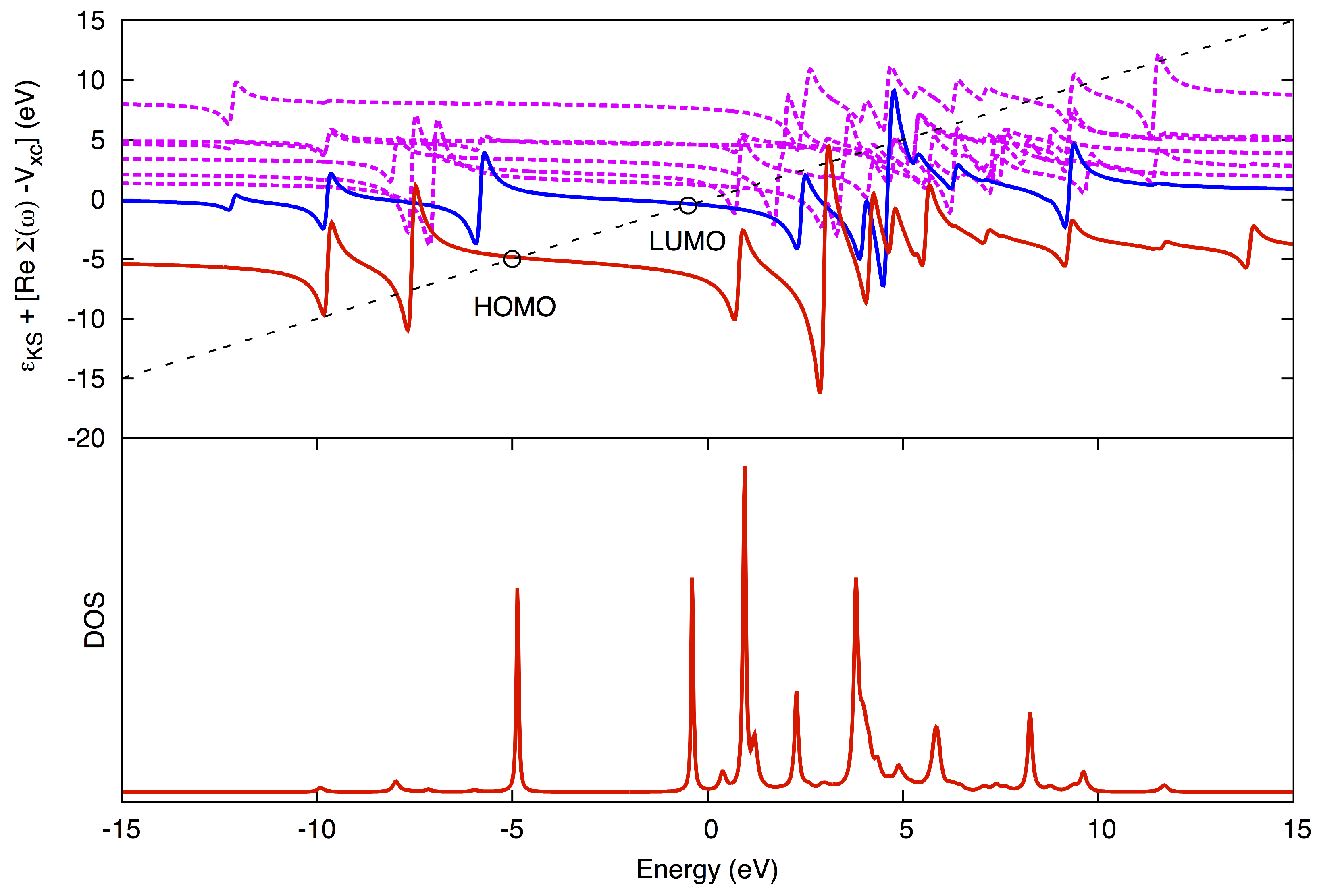
The second way of estimating IPs and EAs is referred to in this paper as the quasiparticle (QP) method. It assumes that the starting MOs, ${\psi }_s$, are a good approximation to the final Dyson amplitudes, which is usually the case for solutions with significant pole strength (i.e., when the self-energy varies sufficiently slowly as is typically the case close to the HOMO-LUMO gap). Then,

$${\omega }_s^{\left(\text{QP}\right)}=\langle {\psi }_s|{\widehat{h}}_H|{\psi }_s\rangle +\Re \langle {\psi }_s|{\Sigma }_{xc}^{G_0{W}_0}({\omega }^{\left(\text{QP}\right)})|{\psi }_s\rangle ,$$

(37)

is solved graphically (Figure 2). The advantage of using the QP method over using the DOS method is that the peaks may be more fully resolved and assigned to a corresponding MO, even for higher poles.

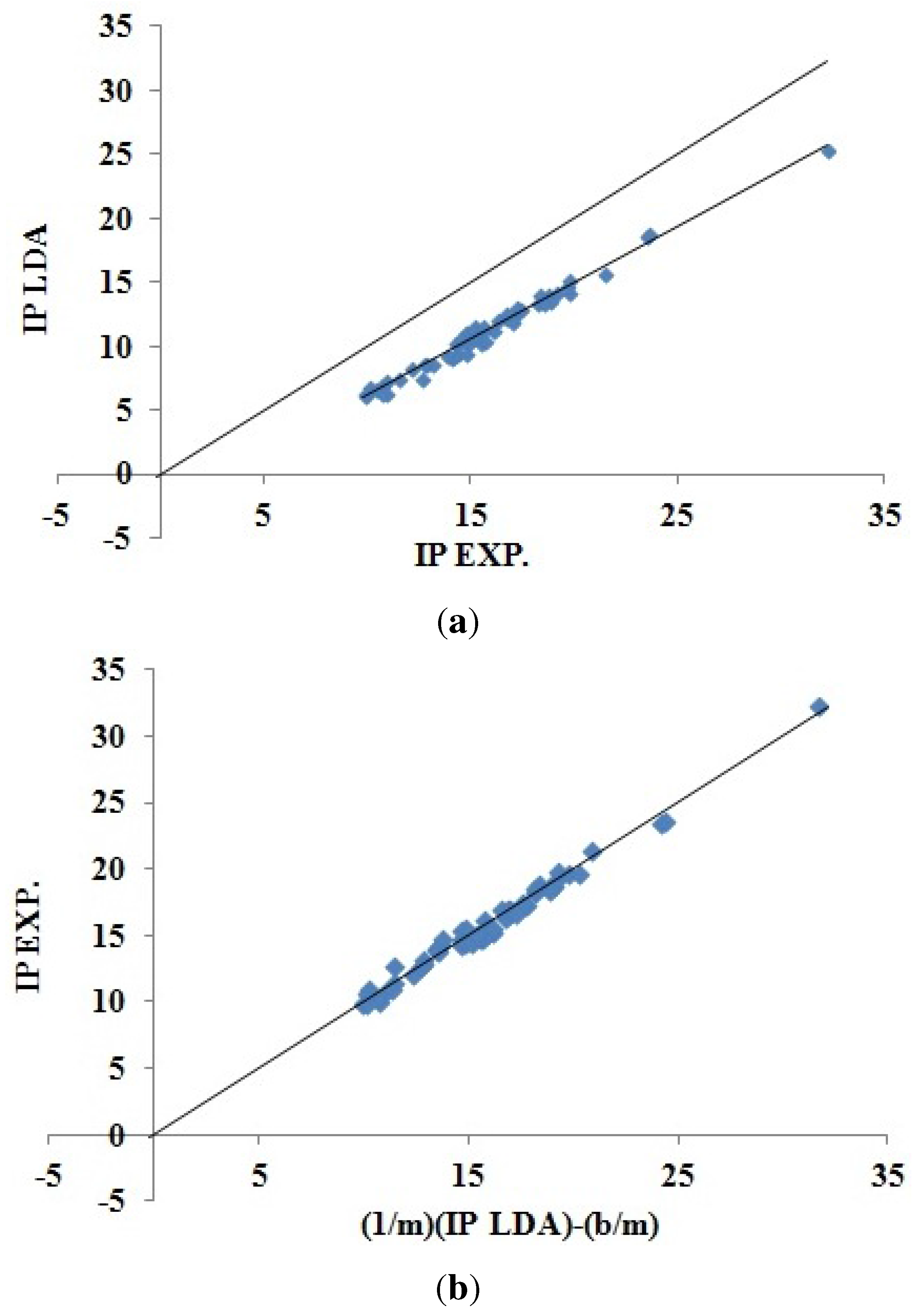
Figure 2. Graphical solution in the quasiparticle (QP) method. (Top) The diagonal line corresponds to ω, while the horizontal curves correspond to $\langle {\psi }_s|{\widehat{h}}_H|{\psi }_s\rangle +\Re \langle {\psi }_s|{\Sigma }_{xc}^{G_0{W}_0}\left(\omega \right)|{\psi }_s\rangle$ for different states, HOMO being red, LUMO blue and higher states jagged magenta. The QP solutions for HOMO and LUMO are marked with circles. (Bottom) The corresponding density-of-states (DOS). Pole strengths (the magnitude of the peaks in the DOS) are obtained from the slope where the diagonal line crosses the horizontal curves.

Figure 2. Graphical solution in the quasiparticle (QP) method. (Top) The diagonal line corresponds to ω, while the horizontal curves correspond to $\langle {\psi }_s|{\widehat{h}}_H|{\psi }_s\rangle +\Re \langle {\psi }_s|{\Sigma }_{xc}^{G_0{W}_0}\left(\omega \right)|{\psi }_s\rangle$ for different states, HOMO being red, LUMO blue and higher states jagged magenta. The QP solutions for HOMO and LUMO are marked with circles. (Bottom) The corresponding density-of-states (DOS). Pole strengths (the magnitude of the peaks in the DOS) are obtained from the slope where the diagonal line crosses the horizontal curves.

4. Small Molecules

In this section and in the next section, we will explain our protocol for assessing DFTB for calculating IPs and EAs and give the results of our assessment. A division has been made between small molecules (this section) and medium-sized molecules (next section). This is because much more information is available for benchmarking small molecules while reliable information for benchmarking medium-sized molecules of interest for organic solar cell applications is much more scarce. In this section, we first review our protocol and illustrate how it works for known results from the literature. We then go on to apply our protocol to the assessment of DFTB calculations.

Benchmark Datasets The identification and tabulation of reliable comparison data are key parts of the test cycle part of the development and successful implementation of a theoretical model for practical applications. The very important and, indeed essential, work involved in establishing such “benchmark datasets” (BDSs) can be substantial and relatively thankless, as it may be regarded primarily as “literature work”, rather than as “new science.” An especially well-known example of such a test set is Charlette E. Moore’s tables of atomic spectra, now freely available from the American National Institute of Standards and Technology (NIST, [81]), which has proven essential in testing different approaches to quantum chemistry.

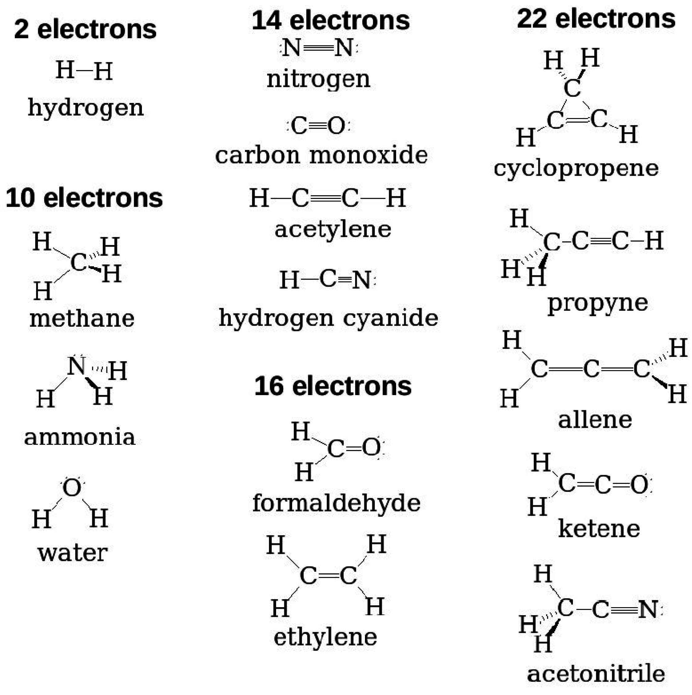
For small molecules, experimental and quantum chemistry ionization potentials (IPs) are readily available from the NIST Computational Chemistry Comparison and Benchmark Database (CCCBDB, [82]). As we have chosen to use the same BDS as in previous work by Hamel et al. [40] for the molecules shown in Figure 3, we have simply taken their values for our small-molecule BDS. This gives a total of 56 IPs (Table 1 and Table 2). Note that these small molecules cannot be used to benchmark electron affinities (EAs) in the sense that most do not bind an extra electron. Hence, we will not assess the quality of DFTB EAs for these small molecules.

Figure 3. The 15 small molecules treated here.

Figure 3. The 15 small molecules treated here.

Analytical Protocol Figure 4 simply takes the data from Hamel et al. [40] to make a correlation plot of minus LDA orbital energies (LDA “Koopmans’ theorem IPs”) versus experimental IPs. It is clear that the LDA Koopmans’ theorem IPs underestimate the experimental IPs, but that also there is an excellent linear correlation between the LDA Koopmans’ theorem IPs and the experimental IPs for these small molecules. We are thus faced with a dilemma regarding how good LDA Koopmans’ IPs are as a model for experimental IPs, and the same dilemma may arise when trying to assess other methods. At this point, we may adapt one of two different quantum chemical philosophies, which Coulson has famously called “Group I” and “Group II” [83] (see also [84,85]). Roughly speaking, Group I focuses on getting good numbers for individual molecules, so that the best theory would have a slope m near unity and an intercept b near zero, while Group II focuses on the ability to predict trends, so that the best theory is one where there is a systematic and, hence, predictive correlation between theory and experiment, even if the two give quantitatively different results.

Table 1. DFTB+ ionization potentials (IPs) (eV) for small molecules. SCC, self-consistent charge.

Molecule	Orbital	Experiment ${}^a$	Without SCC		With SCC
			$-{ϵ}_{\mathbf{i}}$	ΔSCF	$-{ϵ}_{\mathbf{i}}$	ΔSCF
2 electrons
hydrogen (H${}_2$)	$1a_g$	15.43	9.26	9.26	9.26	14.67
10 electrons
methane (CH${}_4$)	$1t_2$	14.3	9.17	9.17	9.00	13.41
ammonia (NH${}_3$)	$3a_1$	10.7	7.73	7.73	6.95	12.18
water (H${}_2$O)	$1b_1$	12.62	9.04	9.04	7.64	13.31
	$3a_1$	14.74	10.28	-	9.03	-
	$1b_2$	18.51	12.31	-	11.54	-
	$2a_1$	32.2	24.65	-	23.48	-
14 electrons
nitrogen (N${}_2$)	$3{\sigma }_g$	15.6	9.70	9.70	9.70	15.33
	$1\pi$	16.98	11.16	-	11.16	-
	$2{\sigma }_u$	18.78	13.98	-	13.98	-
carbon monoxide (CO)	$5\sigma$	14.01	9.16	9.16	9.16	14.47
	$1\pi$	16.91	11.21	-	11.18	-
	$4\sigma$	19.72	13.67	-	13.64	-
acetylene (C${}_2$H${}_2$)	$1{\pi }_u$	11.49	8.33	8.33	7.86	12.23
	$3{\sigma }_g$	16.7	10.29	-	10.11	-
	$2{\sigma }_u$	18.7	12.66	-	12.45	-
	$2{\sigma }_g$	23.5	17.87	-	17.44	-
hydrogen cyanide (HCN)	$1\pi$	13.8	9.79	9.79	9.30	14.12
	$5\sigma$	14.15	9.84	-	9.31	-
	$4\sigma$	19.68	12.42	-	13.11	-
16 electrons
formaldehyde (CH${}_2$O)	$2b_2$	10.9	7.06	7.06	6.43	10.98
	$1b_1$	14.5	10.47	-	9.92	-
	$5a_1$	16.1	10.78	-	10.37	-
	$1b_2$	17.	11.08	-	10.96	-
	$4a_1$	21.4	14.56	-	14.43	-
ethylene (C${}_2$H${}_4$)	$1b_{2u}$	10.68	7.75	7.75	7.36	10.94
	$1b_{2g}$	12.79	8.10	-	7.88	-
	$3a_g$	14.8	9.65	-	9.35	-
	$1b_{3u}$	15.18	10.37	-	10.09	-
	$2b_{1u}$	19.1	13.20	-	12.91	-
	$2a_g$	23.59	17.60	-	17.24	-

${}^a$ Taken from [40].

Table 1. DFTB+ ionization potentials (IPs) (eV) for small molecules. SCC, self-consistent charge.

Molecule	Orbital	Experiment ${}^a$	Without SCC		With SCC
			$-{ϵ}_{\mathbf{i}}$	ΔSCF	$-{ϵ}_{\mathbf{i}}$	ΔSCF
2 electrons
hydrogen (H${}_2$)	$1a_g$	15.43	9.26	9.26	9.26	14.67
10 electrons
methane (CH${}_4$)	$1t_2$	14.3	9.17	9.17	9.00	13.41
ammonia (NH${}_3$)	$3a_1$	10.7	7.73	7.73	6.95	12.18
water (H${}_2$O)	$1b_1$	12.62	9.04	9.04	7.64	13.31
	$3a_1$	14.74	10.28	-	9.03	-
	$1b_2$	18.51	12.31	-	11.54	-
	$2a_1$	32.2	24.65	-	23.48	-
14 electrons
nitrogen (N${}_2$)	$3{\sigma }_g$	15.6	9.70	9.70	9.70	15.33
	$1\pi$	16.98	11.16	-	11.16	-
	$2{\sigma }_u$	18.78	13.98	-	13.98	-
carbon monoxide (CO)	$5\sigma$	14.01	9.16	9.16	9.16	14.47
	$1\pi$	16.91	11.21	-	11.18	-
	$4\sigma$	19.72	13.67	-	13.64	-
acetylene (C${}_2$H${}_2$)	$1{\pi }_u$	11.49	8.33	8.33	7.86	12.23
	$3{\sigma }_g$	16.7	10.29	-	10.11	-
	$2{\sigma }_u$	18.7	12.66	-	12.45	-
	$2{\sigma }_g$	23.5	17.87	-	17.44	-
hydrogen cyanide (HCN)	$1\pi$	13.8	9.79	9.79	9.30	14.12
	$5\sigma$	14.15	9.84	-	9.31	-
	$4\sigma$	19.68	12.42	-	13.11	-
16 electrons
formaldehyde (CH${}_2$O)	$2b_2$	10.9	7.06	7.06	6.43	10.98
	$1b_1$	14.5	10.47	-	9.92	-
	$5a_1$	16.1	10.78	-	10.37	-
	$1b_2$	17.	11.08	-	10.96	-
	$4a_1$	21.4	14.56	-	14.43	-
ethylene (C${}_2$H${}_4$)	$1b_{2u}$	10.68	7.75	7.75	7.36	10.94
	$1b_{2g}$	12.79	8.10	-	7.88	-
	$3a_g$	14.8	9.65	-	9.35	-
	$1b_{3u}$	15.18	10.37	-	10.09	-
	$2b_{1u}$	19.1	13.20	-	12.91	-
	$2a_g$	23.59	17.60	-	17.24	-

${}^a$ Taken from [40].

Table 2. DFTB+ IPs (eV) for small molecules (continued).

Molecule	Orbital	Experiment ${}^a$	Without SCC		With SCC
			$-{ϵ}_{\mathbf{i}}$	ΔSCF	$-{ϵ}_{\mathbf{i}}$	ΔSCF
22 electrons
cyclopropene (C${}_3$H${}_4$)	$2b_2$	9.86	6.75	6.75	6.28	10.00
	$2b_1$	10.89	7.64	-	7.20	-
	$6a_2$	12.7	8.59	-	8.11	-
	$1b_2$	15.09	10.01	-	9.52	-
	$5a_1$	16.68	10.36	-	10.04	-
	$2b_1$	18.3	13.01	-	12.69	-
	$4a_1$	19.6	13.95	-	13.48	-
propyne (CH${}_3$CCH)	$2e$	10.37	7.71	7.71	7.18	10.87
	$1e$	14.4	9.71	-	9.65	-
	$7a_1$	15.5	10.00	-	9.69	-
	$6a_1$	17.2	11.91	-	11.56	-
allene (C${}_3$H${}_4$)	$2e$	10.02	7.21	7.21	6.85	10.43
	$1e$	14.75	9.95	-	9.67	-
	$3b_2$	14.75	9.98	-	9.68	-
	$4a_1$	17.3	11.93	-	11.66	-
ketene (CH${}_2$CO)	$2b_1$	9.8	6.27	6.27	6.20	10.21
	$2b_2$	14.2	9.24	-	9.23	-
	$1b_1$	15.	10.62	-	10.71	-
	$1b_2$	16.3	10.93	-	10.97	-
	$7a_1$	16.8	11.07	-	11.14	-
	$6a_1$	18.2	12.94	-	12.86	-
acetonitrile (CH${}_3$CN)	$2e$	12.08	8.66	8.66	8.45	12.30
	$7a_1$	13.11	9.69	-	8.96	-
	$1e$	15.5	10.25	-	10.36	-
	$6a_1$	17.4	11.81	-	11.77	-

${}^a$ Taken from [40].

Table 2. DFTB+ IPs (eV) for small molecules (continued).

Molecule	Orbital	Experiment ${}^a$	Without SCC		With SCC
			$-{ϵ}_{\mathbf{i}}$	ΔSCF	$-{ϵ}_{\mathbf{i}}$	ΔSCF
22 electrons
cyclopropene (C${}_3$H${}_4$)	$2b_2$	9.86	6.75	6.75	6.28	10.00
	$2b_1$	10.89	7.64	-	7.20	-
	$6a_2$	12.7	8.59	-	8.11	-
	$1b_2$	15.09	10.01	-	9.52	-
	$5a_1$	16.68	10.36	-	10.04	-
	$2b_1$	18.3	13.01	-	12.69	-
	$4a_1$	19.6	13.95	-	13.48	-
propyne (CH${}_3$CCH)	$2e$	10.37	7.71	7.71	7.18	10.87
	$1e$	14.4	9.71	-	9.65	-
	$7a_1$	15.5	10.00	-	9.69	-
	$6a_1$	17.2	11.91	-	11.56	-
allene (C${}_3$H${}_4$)	$2e$	10.02	7.21	7.21	6.85	10.43
	$1e$	14.75	9.95	-	9.67	-
	$3b_2$	14.75	9.98	-	9.68	-
	$4a_1$	17.3	11.93	-	11.66	-
ketene (CH${}_2$CO)	$2b_1$	9.8	6.27	6.27	6.20	10.21
	$2b_2$	14.2	9.24	-	9.23	-
	$1b_1$	15.	10.62	-	10.71	-
	$1b_2$	16.3	10.93	-	10.97	-
	$7a_1$	16.8	11.07	-	11.14	-
	$6a_1$	18.2	12.94	-	12.86	-
acetonitrile (CH${}_3$CN)	$2e$	12.08	8.66	8.66	8.45	12.30
	$7a_1$	13.11	9.69	-	8.96	-
	$1e$	15.5	10.25	-	10.36	-
	$6a_1$	17.4	11.81	-	11.77	-

${}^a$ Taken from [40].

In the spirit of Group I, we should keep in mind that even the best computed molecular vertical IPs have an average error of about 0.2 eV compared to experimental vertical IPs determined by peak maxima in photoelectron spectra, because of the neglect of vibrational (i.e., Franck–Condon) effects. In the spirit of Group II, we have taken the standard error,

$$\Delta y=\sqrt{\frac{{\mathcal{E}}_y}{N-2}}$$

(38)

where,

$${\mathcal{E}}_y=\sum _{i=1,N}{\left(y_i-m{x}_i-b\right)}^2$$

(39)

as the most transferable estimate of the goodness of the fit. However, if we now take the fit values of m and b found above for a particular method and then use them in the formula,

$$x=\frac{1}{m}y-\frac{b}{m}$$

(40)

to try to estimate the error in the predicted value of BDS values corresponding to the results of the model, then the relevant standard error is:

$$\Delta x=\sqrt{\frac{{\mathcal{E}}_x}{N-2}}=\frac{\Delta y}{\left|m\right|},$$

(41)

where:

$${\mathcal{E}}_x=\sum _{i=1,N}{\left(x_i-\frac{1}{m}{y}_i+\frac{b}{m}\right)}^2=\frac{{\mathcal{E}}_y}{m^2}.$$

(42)

Thus, $\Delta x$ is the relevant measure of the predictability of a given model.

Figure 4. (a) Correlation plot for LDA “Koopmans’ theorem IPs” versus experimental IPs [40]; (b) inversion plot for the same data constructed using Equation (40) to show the “predictive ability” of the LDA least squares fit. The units for both axes in these plots are eV.

Figure 4. (a) Correlation plot for LDA “Koopmans’ theorem IPs” versus experimental IPs [40]; (b) inversion plot for the same data constructed using Equation (40) to show the “predictive ability” of the LDA least squares fit. The units for both axes in these plots are eV.

The results of a statistical analysis of the results in [40] for least square fits of various theoretical methods to experiments are shown in Table 3 and Table 4. Consistent with Figure 4, Table 3 shows that the DFT LDA Koopmans’ theorem (KT) underestimates by 4–6 eV (i.e., $y-x=(m-1)x+b$ is −3.87 eV at $x=$ 10. eV and −6.23 eV at $x=$ 30. eV) and, so, is a dismal failure from the point of view of Coulson Group I. This has been explained in terms of the particle number discontinuity in the DFT exchange-correlation (xc) potential [86]. The Hartree–Fock (HF) KT IPs are better from the point of view of Coulson Group I, but tend to slightly overestimate the experimental IPs. This is consistent with early literature, which proposed as a rule of thumb that agreement between HF KT and photoelectron spectroscopy (PES) IPs could be improved by multiplying the HF KT values by a factor of less than one (e.g., 0.92 or the “8% rule” [87,88]). Surprisingly, localizing the HF exchange operator by the optimized effective, potential method (OEP) so as to obtain an exact exchange-only xc-potential which includes a derivative discontinuity, leads to much improved absolute agreement between KT and experimental IPs with a slightly reduced standard error ($\Delta y$). Part of the reason for the smaller value of $\Delta y$ is that the OEP corrects misorderings in the KT IPs, which are present when KT is used with the nonlocal HF exchange operator. Note that the OEP procedure makes use of the constraint that the highest occupied molecular orbital (HOMO) energy be identical for HF and OEP when both are evaluated with the OEP orbitals [41]. Thus, the OEP HOMO energy is almost, but not exactly, the same as the HF HOMO energy.

Table 3. Fitting data for outer valence IPs: $y=mx+b$, where x is the experimental IP and y is the calculated IP, both in eV. HF, Hartree–Fock; OEP, optimized effective potential; LDA, local density approximation; DFTB, density-functional tight binding (without self-consistent charge); SCC-DFTB, self-consistent charge DFTB.

Method	m (Unitless)	b (eV)	$\Delta y$ (eV)	$\Delta x$ (eV)
Koopmans’ Theorem
OEP ${}^a$	0.958	0.748	0.659	0.688
HF ${}^a$	1.236	−2.192	0.686	0.555
LDA ${}^a$	0.882	−2.691	0.474	0.537
DFTB ${}^b$	0.754	−1.071	0.651	0.863
SCC-DFTB ${}^b$	0.758	−1.442	0.535	0.706
ΔSCF
LDA ${}^c$	1.65	2.54	1.65	1.85

${}^a$ Calculated from data in [40]; ${}^b$ present work; ${}^c$ approximate ΔSCF values calculated using Slater’s transition orbital method. “rTS” (restricted transition state) values from [89].

Table 3. Fitting data for outer valence IPs: $y=mx+b$, where x is the experimental IP and y is the calculated IP, both in eV. HF, Hartree–Fock; OEP, optimized effective potential; LDA, local density approximation; DFTB, density-functional tight binding (without self-consistent charge); SCC-DFTB, self-consistent charge DFTB.

Method	m (Unitless)	b (eV)	$\Delta y$ (eV)	$\Delta x$ (eV)
Koopmans’ Theorem
OEP ${}^a$	0.958	0.748	0.659	0.688
HF ${}^a$	1.236	−2.192	0.686	0.555
LDA ${}^a$	0.882	−2.691	0.474	0.537
DFTB ${}^b$	0.754	−1.071	0.651	0.863
SCC-DFTB ${}^b$	0.758	−1.442	0.535	0.706
ΔSCF
LDA ${}^c$	1.65	2.54	1.65	1.85

${}^a$ Calculated from data in [40]; ${}^b$ present work; ${}^c$ approximate ΔSCF values calculated using Slater’s transition orbital method. “rTS” (restricted transition state) values from [89].

Table 4. Fitting data for first IPs [40]: $y=mx+b$, where x is the experimental IP and y is the theoretical IP, both in eV. HF, Hartree–Fock; OEP, optimized effective potential; LDA, local density approximation; DFTB, density-functional tight binding (without self-consistent charge); SCC-DFTB, self-consistent charge DFTB.

Method	m (Unitless)	b (eV)	$\Delta y$ (eV)	$\Delta x$ (eV)
Koopmans’ Theorem
HF ${}^a$	1.143	−1.270	0.617	0.540
OEP ${}^a$	1.145	−1.294	0.613	0.535
LDA ${}^a$	0.727	−1.064	0.374	0.514
DFTB ${}^b$	0.497	2.223	0.498	1.002
SCC-DFTB ${}^b$	0.560	1.064	0.477	0.852
ΔSCF
LDA ${}^c$	1.00	0.49	0.43	0.43
DFTB ${}^b$	0.497	2.223	0.498	1.002
SCC-DFTB ${}^b$	0.838	2.239	0.534	0.649

${}^a$ Calculated from data in [40]; ${}^b$ present work. ${}^c$ approximate ΔSCF values calculated using Slater’s transition orbital method. “rTS” values from [89].

Table 4. Fitting data for first IPs [40]: $y=mx+b$, where x is the experimental IP and y is the theoretical IP, both in eV. HF, Hartree–Fock; OEP, optimized effective potential; LDA, local density approximation; DFTB, density-functional tight binding (without self-consistent charge); SCC-DFTB, self-consistent charge DFTB.

Method	m (Unitless)	b (eV)	$\Delta y$ (eV)	$\Delta x$ (eV)
Koopmans’ Theorem
HF ${}^a$	1.143	−1.270	0.617	0.540
OEP ${}^a$	1.145	−1.294	0.613	0.535
LDA ${}^a$	0.727	−1.064	0.374	0.514
DFTB ${}^b$	0.497	2.223	0.498	1.002
SCC-DFTB ${}^b$	0.560	1.064	0.477	0.852
ΔSCF
LDA ${}^c$	1.00	0.49	0.43	0.43
DFTB ${}^b$	0.497	2.223	0.498	1.002
SCC-DFTB ${}^b$	0.838	2.239	0.534	0.649

${}^a$ Calculated from data in [40]; ${}^b$ present work. ${}^c$ approximate ΔSCF values calculated using Slater’s transition orbital method. “rTS” values from [89].

The outlook changes dramatically from the point of view of Coulson Group II. Looking at $\Delta x$ in Table 3 and Table 4, we see that the LDA KT provides as much predictability (indeed somewhat more) as either the HF or OEP KT, indicating that, although shifted, the LDA KT IPs provide an excellent reflection of the trend in the experimental IPs. Closer analysis of why the LDA results are a bit better than the HF or OEP (smaller $\Delta x$) shows that the LDA KT IPs have fewer order reversals compared to experimental IPs than do the HF KT IPs. This also occurs when the HF exchange potential is localized in the OEP procedure, though $\Delta x$ is larger for the OEP calculations than for the HF calculations, indicating decreasing predictability upon localization. The above trends do not seem to be well known to most users of quantum chemistry programs, but this does not seem to be the place to spend time and space giving further details (see [41] for an additional discussion). Suffice it to say that the above information is “well-known to those who know about such things” and that further information is contained in the cited papers. It should also be evident that global hybrid functionals containing a nonzero amount of HF exchange will have a behavior in between the LDA and HF, as can be easily checked using information from the NIST CCCBDB, but we shall not pursue this topic further here.

Assessment of DFTB The results of our DFTB+ calculations of IPs and EAs are shown in Table 1 and Table 2. The results of a statistical analysis of our DFTB results relative to experiments are also shown in Table 3 and Table 4.

Since DFTB has been designed as an approximation on DFT, we expect DFTB to behave in much the same way, albeit not exactly, as DFT. We also expect the SCC option to give results closer to DFT than results without the SCC. Let us verify that this is true by first looking at calculations without the SCC option. A trivial consequence of the basic theory (previous section) is that the ΔSCF and Koopmans’ theorem IPs are identical for the original DFTB method, and our results confirm this. Figure 5 shows how DFTB Koopmans’ theorem IPs correlate with experiment. As we would hope, this figure is remarkably similar to the corresponding LDA figure (Figure 4). The DFTB Koopmans’ theorem IPs are underestimates of the experimental IPs in much the same way as the LDA underestimates Koopmans’ theorem. This is consistent with DFTB having been constructed to behave like DFT; a conclusion that is confirmed by Figure 6 showing the excellent correlation between DFTB and LDA Koopmans’ theorem IPs. In spite of the similarity of the graphics, the LDA and DFTB values of $\Delta x$ in Table 3 are a reminder that DFTB is significantly less predictive (error bar of ±0.863 eV) than is the LDA (error bar of ±0.537 eV).

Figure 5. Correlation plot for DFTB “Koopmans’ theorem IPs” versus experimental IPs. (a) Correlation plot for DFTB “Koopmans’ theorem IPs” versus experimental IPs; (b) inversion plot for the same data constructed using Equation (40) to show the “predictive ability” of the DFTB least squares fit. The units for both axes in these plots are in eV.

Figure 5. Correlation plot for DFTB “Koopmans’ theorem IPs” versus experimental IPs. (a) Correlation plot for DFTB “Koopmans’ theorem IPs” versus experimental IPs; (b) inversion plot for the same data constructed using Equation (40) to show the “predictive ability” of the DFTB least squares fit. The units for both axes in these plots are in eV.

Figure 6. Correlation plot for DFTB versus LDA “Koopmans’ theorem IPs.” The units for both axes are eV.

Figure 6. Correlation plot for DFTB versus LDA “Koopmans’ theorem IPs.” The units for both axes are eV.

According to Table 3 and Table 4, including SCC in DFTB leads to a significant partial improvement. While SCC-DFTB still behaves much like the LDA, SCC-DFTB Koopmans’ theorem IPs are more predictive (error bar of ± 0.706 eV) than DFTB Koopmans’ theorem IPs, though still less than LDA Koopmans’ theorem IPs. If we restrict attention to the HOMO, than we can also compare Koopmans’ theorem to ΔSCF SCC-DFTB (which we recall are the same in the case without the SCC). Here, we see that the ΔSCF method provides more predictive ability than does the Koopmans’ theorem approach. In fact, the SCC-DFTB ΔSCF error bar (± 0.649 eV) is becoming encouragingly close to the LDA Koopmans’ theorem error bar (± 0.514 eV), although it is still not as small as that of the “rTS” estimate of the LDA ΔSCF IPs (± 0.43 eV) whose calculation were reported in [89].

5. Medium-Sized Molecules

The small molecules in the previous section provide a good idea of how various methods work for calculating IPs for such systems. In particular, we confirmed DFTB much like DFT and placed error bars on the predictive power of the method. Thus, for small molecules, DFT (or some other first-principles method) is preferable to DFTB. However, our interest is in organic electronics, where interesting molecules, and their assembly into realistic systems, rapidly leads to calculations, which are difficult to attack any other way, except using a semi-empirical method, such as DFTB. It is important to see to what extent that what we have learned for small molecules also applies to larger molecules of more interest for organic electronics. This is especially true, since methods tested and found to work well for small molecules do not always perform equally well for large molecules [26]. In this section, we focus on assessing DFTB for the calculation of IPs and EAs for a BDS of “medium-sized” molecules often used in organic electronics (Figure 1).

Choice of Comparison Data Of course, the notion of “small,” “medium” and “large” is not well-defined. In the present context, molecules are “medium sized” in the sense that they are the smallest molecules of interest for organic electronics, and yet, they are already too large for the NIST CCBDB, which is limited to species with no more than 26 atoms total. Our medium-sized molecules are also large enough that it is experimentally more natural to treat them either in the bulk phase, as either a thin film or in solution electrochemistry, than in the gas phase, though gas phase molecular data are available for a number of the molecules. IPs and EAs for these molecules are frequently determined by thin-film photoelectron or photoemission spectroscopy or by cyclic voltammetry and involve a certain number of assumptions whose accuracy is not always easy to assess. In particular, in thin film photoelectron and photoemission spectroscopy, the difference between the ionization energy of the molecule and the bulk is sometimes referred to as “the polarization energy due to the molecular ion left in the solid after a photoelectron is removed” [90], which is a quantity that is not evident to calculate. Furthermore, the relationship between the bulk ultraviolet photoemission spectroscopy ionization energy and the oxidation potential of cyclic voltammetry requires a model in which it is assumed that the molecules form a thin film on the electrodes similar to that found in the bulk [91], which is also not easy to model theoretically. Because of these complications, we place our trust more firmly in gas phase results, where available, than in bulk phase results. Furthermore, as we shall see, reliable theoretical calculations are possible for the gas phase. Thus, once validated by comparison against gas phase data, we may use appropriate theoretical methodology to obtain a BDS of IPs and EAs.

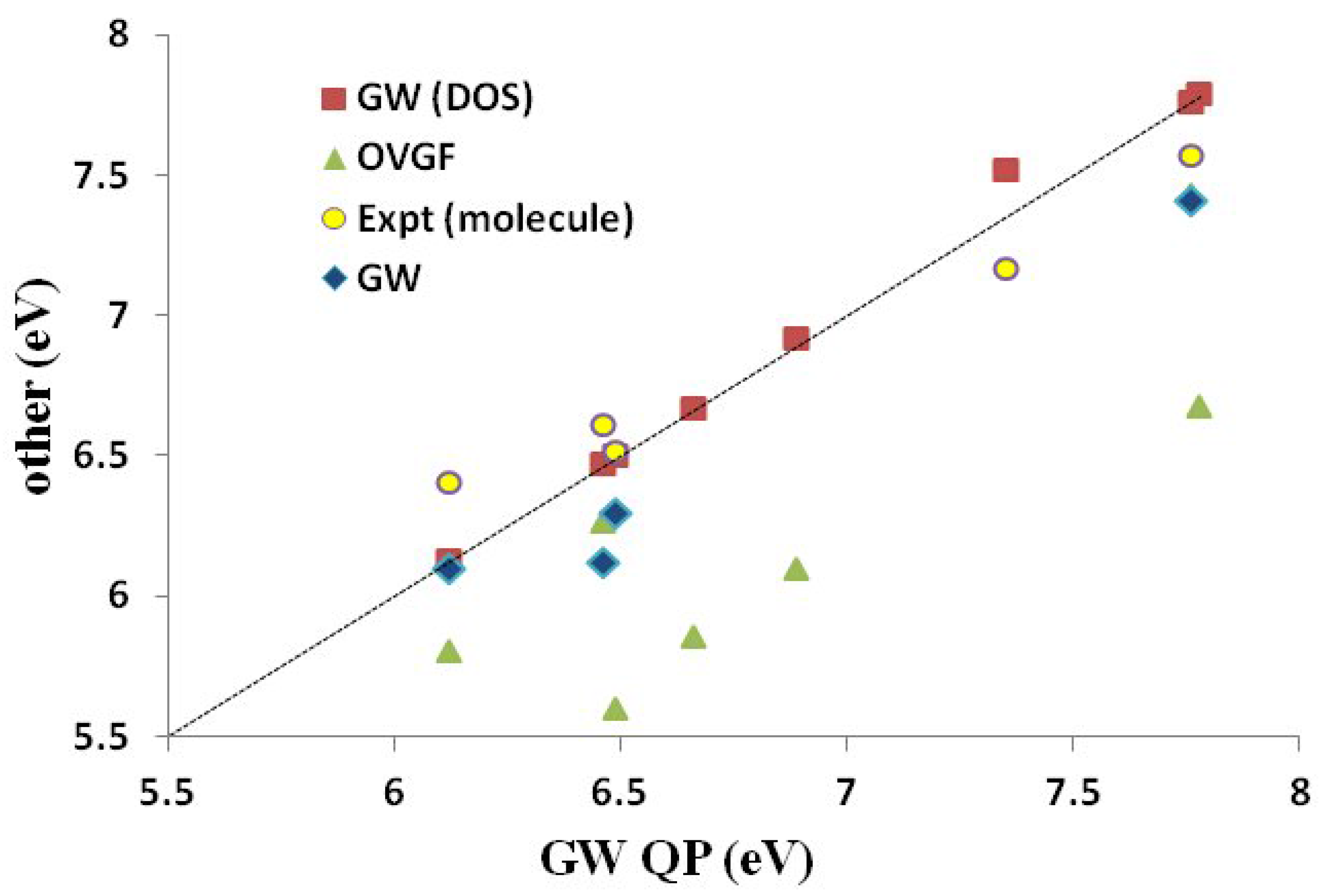
Assessment of Our $GW$ Calculations Table 5 and Figure 7 show how various Green’s function calculations compare to experimental data for predicting IPs. It is immediately obvious that the experimental molecular (gas phase) IPs are in much better agreement with the Green’s function IPs than are experimental bulk (solution or thin film) IPs. This is, of course, to be expected on the basis of the above discussion. Of the different sets of Green’s function IPs, our OVGF values are in the worst agreement with the experimental molecular IPs. As stated earlier (Section 3), we believe that this is simply because we were unable to carry out OVGF calculations with extensive basis sets. Both our $GW$ DOS and $GW$ QP IPs agree as well, or better than, with the available experimental molecular IPs as do the $GW$ IPs taken from the literature. In the one case (PCBM) where a significant difference was observed between our $GW$ DOS and $GW$ QP IPs, it is the $GW$ QP IPs that are closer to the available experimental molecular value. This is because the DOS approach failed due to the HOMO level being smeared by the three nearly degenerate levels HOMO-1, HOMO-2 and HOMO-3.

Reliable experimental EA comparison data for molecules of interest in organic electronics is even harder to come across than for IPs. There are several reasons for this. Some are similar to those encountered with IPs, such as the difficulty of obtaining gas phase data. Some are particular to the experimental problem of obtaining electron addition rather than electron removal energies. Thus, our calculated EAs are vertical, while the experimental EAs are often best considered to be adiabatic, because of the experiments used to measure them. Furthermore, it must be remembered that that EAs tend to be smaller than IPs, except in the case of good electron acceptors, such as C${}_{60}$ and PCBM, whose EAs are expected to be so similar that they may be difficult to distinguish by theoretical calculations. 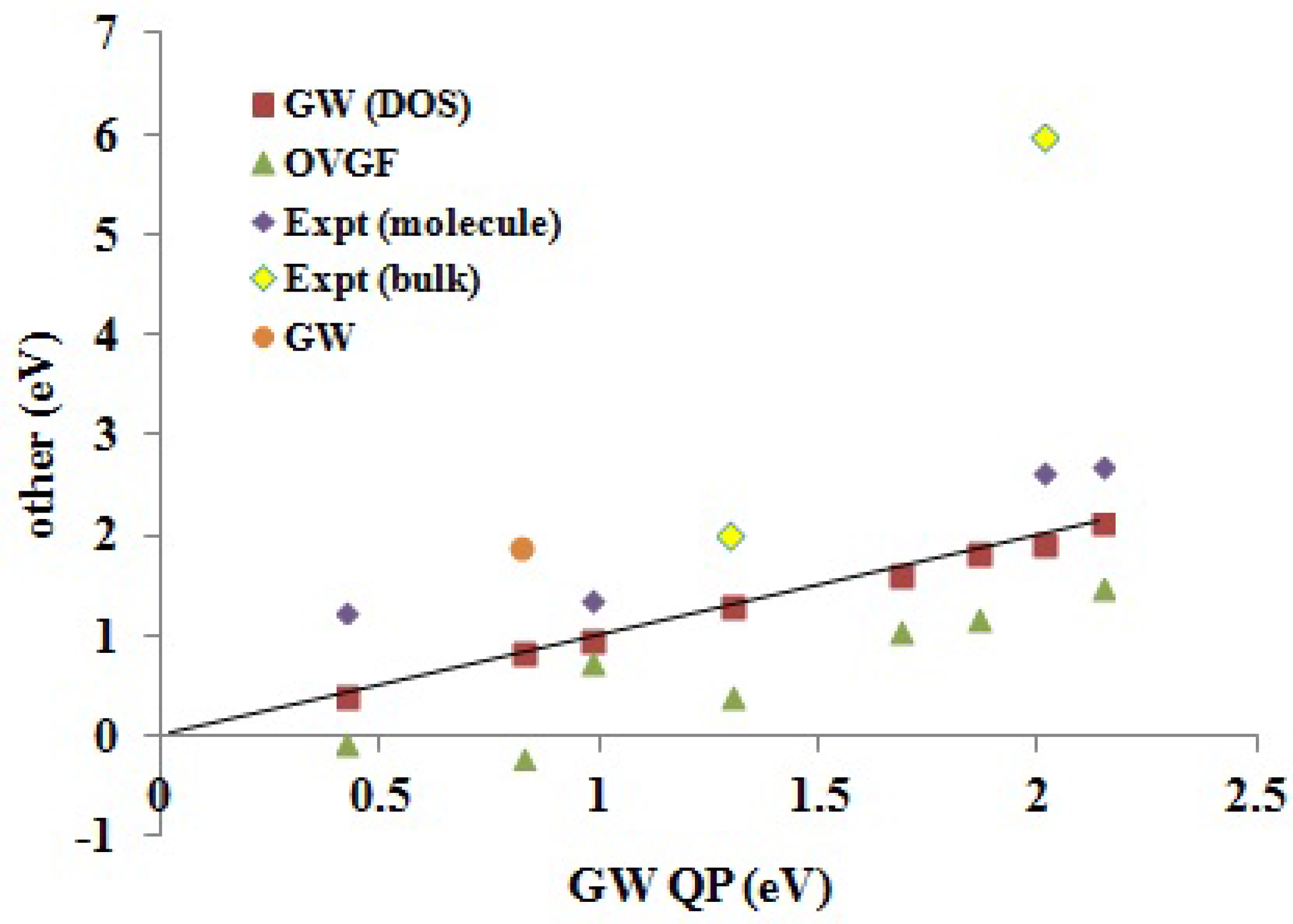Nevertheless, Table 6 and Figure 8 show that our $GW$ EAs also agree well with available experimental molecular (gas phase) data.

Table 5. Comparison values of the first ionization potential for the medium-sized molecules from experiment and from quantum chemistry calculations. OVGF, outer-valence Green’s function.

Molecule	Experiment		Green’s Function
	Bulk	Molecule	OVGF	GW
				PW		Literature
				DOS ${}^{\mathit{p}}$	QP ${}^{\mathit{q}}$
pentacene		6.61 e	5.78 ${}^b$	6.47	6.46	6.12 ${}^d$
			6.27 ${}^c$
DIP	5.35 ${}^m$		6.10 ${}^b$	6.91	6.89
H${}_2$Pc		6.41 ${}^f$	5.81 ${}^b$	6.13	6.12	6.10 ${}^d$
PCBM	5.87 ${}^h$	7.17 ${}^n$		7.52	7.35
6T	4.7 ${}^m$		5.86 ${}^b$	6.67	6.66
DCV3T	6.09 ${}^a$		6.68 ${}^b$	7.79	7.78
C${}_{60}$	6.45 ${}^m$	7.57 ${}^g$	7.43 ${}^b$	7.76	7.76	7.41 ${}^d$
rubrene	5.92 ${}^i$	6.52 ${}^i$	5.60 ${}^b$	6.50	6.49	6.30 ${}^l$
Molecule	Koopmans’ Theorem				ΔSCF
	HF	B3LYP o	DFTB	SCC-	B3LYP o	SCC-
				DFTB		DFTB
pentacene	5.91 ${}^j$	4.59	5.38	4.97	5.93	6.81
	6.09 ${}^k$
DIP	6.54 ${}^j$	5.12	5.73	5.35	6.32	6.99
H${}_2$Pc	5.47 ${}^j$	4.93	5.14	4.96	6.05	6.49
PCBM		5.65	5.48	5.38	6.81	7.01
6T	6.46 ${}^j$	4.82	5.17	4.79	5.88	6.22
DCV3T	7.62 ${}^j$	6.01	5.40	5.64	7.10	7.21
C${}_{60}$	7.95 ${}^j$	5.98	5.67	5.67	7.22	7.41
rubrene	6.08 ${}^j$	4.67	5.36	4.90	5.85	6.59

${}^a$ Estimated from cyclic voltammetry in CH${}_2$Cl${}_2$ [92]. ${}^b$ Present work: OVGF/6-31G//B3LYP/6-31G**. ${}^c$ Present work: OVGF/6-311++G**//B3LYP/6-31G**. ${}^d$ $GW$ from Table II of [36]. e Gas-phase charge-stripping mass spectroscopy [93]. ${}^f$ Gas-phase photoelectron spectroscopy (PES) [94]. ${}^g$ From [95]. ${}^h$ Thin-film ultraviolet photoemission spectroscopy (UPS) [96]. ${}^i$ Gas and thin-film photoelectron spectroscopy (PES) [90]. ${}^j$ Present work: HF/6-31G//B3LYP/6-31G**. ${}^k$ Present work: HF/6-311++G**//B3LYP/6-31G**. ${}^l$ From [97]. ${}^m$ Ultraviolet photoemission spectroscopy (UPS) [98]. ${}^n$ [99]. o Present work: B3LYP/6-31G*//B3LYP/6-31G*. ${}^p$ Present work: inspection of the density of states. ${}^q$ Present work: solution of the quasiparticle equation.

Table 5. Comparison values of the first ionization potential for the medium-sized molecules from experiment and from quantum chemistry calculations. OVGF, outer-valence Green’s function.

Molecule	Experiment		Green’s Function
	Bulk	Molecule	OVGF	GW
				PW		Literature
				DOS ${}^{\mathit{p}}$	QP ${}^{\mathit{q}}$
pentacene		6.61 e	5.78 ${}^b$	6.47	6.46	6.12 ${}^d$
			6.27 ${}^c$
DIP	5.35 ${}^m$		6.10 ${}^b$	6.91	6.89
H${}_2$Pc		6.41 ${}^f$	5.81 ${}^b$	6.13	6.12	6.10 ${}^d$
PCBM	5.87 ${}^h$	7.17 ${}^n$		7.52	7.35
6T	4.7 ${}^m$		5.86 ${}^b$	6.67	6.66
DCV3T	6.09 ${}^a$		6.68 ${}^b$	7.79	7.78
C${}_{60}$	6.45 ${}^m$	7.57 ${}^g$	7.43 ${}^b$	7.76	7.76	7.41 ${}^d$
rubrene	5.92 ${}^i$	6.52 ${}^i$	5.60 ${}^b$	6.50	6.49	6.30 ${}^l$
Molecule	Koopmans’ Theorem				ΔSCF
	HF	B3LYP o	DFTB	SCC-	B3LYP o	SCC-
				DFTB		DFTB
pentacene	5.91 ${}^j$	4.59	5.38	4.97	5.93	6.81
	6.09 ${}^k$
DIP	6.54 ${}^j$	5.12	5.73	5.35	6.32	6.99
H${}_2$Pc	5.47 ${}^j$	4.93	5.14	4.96	6.05	6.49
PCBM		5.65	5.48	5.38	6.81	7.01
6T	6.46 ${}^j$	4.82	5.17	4.79	5.88	6.22
DCV3T	7.62 ${}^j$	6.01	5.40	5.64	7.10	7.21
C${}_{60}$	7.95 ${}^j$	5.98	5.67	5.67	7.22	7.41
rubrene	6.08 ${}^j$	4.67	5.36	4.90	5.85	6.59

${}^a$ Estimated from cyclic voltammetry in CH${}_2$Cl${}_2$ [92]. ${}^b$ Present work: OVGF/6-31G//B3LYP/6-31G**. ${}^c$ Present work: OVGF/6-311++G**//B3LYP/6-31G**. ${}^d$ $GW$ from Table II of [36]. e Gas-phase charge-stripping mass spectroscopy [93]. ${}^f$ Gas-phase photoelectron spectroscopy (PES) [94]. ${}^g$ From [95]. ${}^h$ Thin-film ultraviolet photoemission spectroscopy (UPS) [96]. ${}^i$ Gas and thin-film photoelectron spectroscopy (PES) [90]. ${}^j$ Present work: HF/6-31G//B3LYP/6-31G**. ${}^k$ Present work: HF/6-311++G**//B3LYP/6-31G**. ${}^l$ From [97]. ${}^m$ Ultraviolet photoemission spectroscopy (UPS) [98]. ${}^n$ [99]. o Present work: B3LYP/6-31G*//B3LYP/6-31G*. ${}^p$ Present work: inspection of the density of states. ${}^q$ Present work: solution of the quasiparticle equation.

Figure 7. Correlation graph of data from Table 5 showing how experimental and Green’s function IPs compare. The label “$GW$” (as opposed to $GW$ DOS and $GW$ QP) is the calculated values taken from the literature (see Table 5). Units are in eV. The x-axis corresponds to our $GW$ QP calculations.

Figure 7. Correlation graph of data from Table 5 showing how experimental and Green’s function IPs compare. The label “$GW$” (as opposed to $GW$ DOS and $GW$ QP) is the calculated values taken from the literature (see Table 5). Units are in eV. The x-axis corresponds to our $GW$ QP calculations.

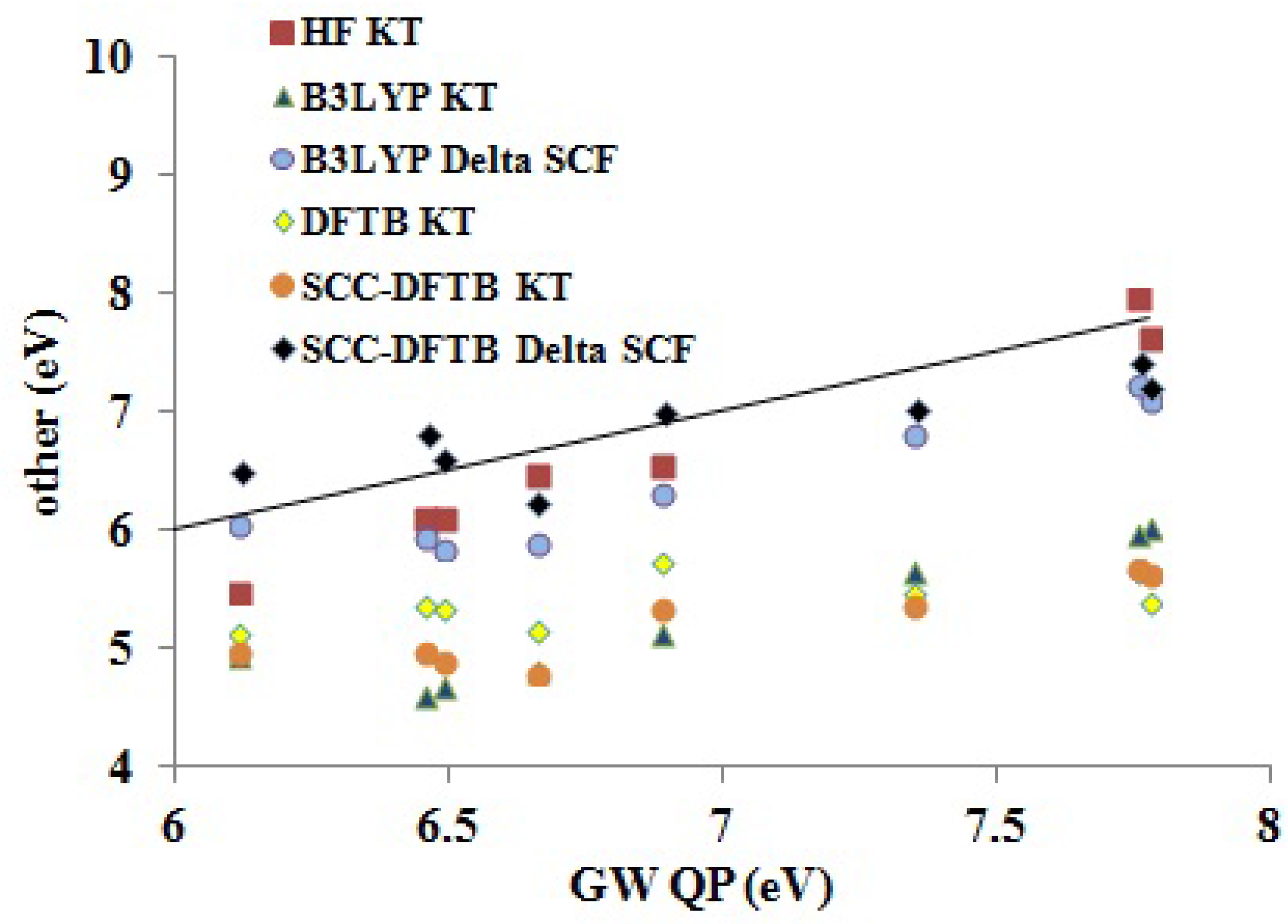
In conclusion, we feel justified in using our $GW$ QP values of IPs and EAs as a BDS for medium-sized molecules. We will use these to judge the quality of DFTB IPs and EAs.

Assessment of Our DFTB Calculations Figure 9 shows how DFTB and other approximate theoretical methods compare to our $GW$ QP IP BDS. Fitting data, including $\Delta y$ and $\Delta x$ values, are shown in Table 7. In general, the HF KT and the ΔSCF methods give the best absolute agreement with the $GW$ QP results. Somewhat surprisingly, the HF KT IPs underestimate the GW QP IPs, though HF KT IPs typically overestimate experimental IPs for small molecules. The B3LYP ΔSCF values underestimate the GW QP IPs somewhat more than do the HF KT IPs. The SCC-DFTB ΔSCF are perhaps closer in absolute values to the GW QP IPs, but the trend (slope m in Table 7) is better for the B3LYP ΔSCF ($m=0.856$) than for the SCC-DFTB ΔSCF ($m=0.520$) method. As expected, the B3LYP KT, DFTB KT (the same as DFTB ΔSCF) and SCC-DFTB KT values are shifted down. The trends are best represented by the B3LYP KT ($m=0.867$) method, less so by the SCC-DFTB KT ($m=0.504$) method and very badly by the DFTB KT ($m=0.200$) method. Focusing on $\Delta x$ as a measure of the predictive value, we see that the B3LYP method is most predictive (ΔSCF $\Delta x=0.256$ eV, KT $\Delta x=0.270$ eV), but that the SCC-DFTB method is still fairly good (ΔSCF $\Delta x=0.489$ eV, KT $\Delta x=0.326$ eV). Surprisingly, the SCC-DFTB KT approach seems to have somewhat more predictive power than does the SCC-DFTB ΔSCF method, but we would not count on this always being the case. Of course, the original DFTB is not nearly as good ($\Delta x=0.982$ eV).

Table 6. Comparison values of the first electron affinity for the medium-sized molecules from the experiment and from quantum chemistry calculations.

Molecule	Experiment		Green’s Function
	Bulk	Molecule	OVGF	GW
				PW		Literature
				DOS ${}^{\mathit{p}}$	QP ${}^{\mathit{q}}$
pentacene		1.35 ${}^f$	0.001 ${}^c$	0.985	0.981
			0.755 ${}^d$	0.941	0.953
DIP	2. ${}^g$		0.421 ${}^c$	1.31	1.30
H${}_2$Pc			1.063 ${}^c$	1.64	1.68
PCBM	5.96 ${}^j$	2.63 ${}^n$		1.94	2.01
6T		1.25 ${}^m$	–0.045 ${}^c$	0.413	0.422
DCV3T	3.90 ${}^i$		1.201	1.85	1.86
C${}_{60}$		2.68 ${}^n$	1.486 ${}^c$	2.14	2.14
rubrene			–0.195 ${}^c$	0.839	0.822	1.88 o
Molecule	Koopmans’ Theorem				ΔSCF
	HF	B3LYP e	DFTB	SCC-	B3LYP e	SCC-
				DFTB		DFTB
pentacene	0.553 ${}^k$	2.38	4.05	3.63	1.05	1.80
	−0.274 ${}^l$
DIP	−0.251 ${}^k$	2.59	4.14	3.75	1.39	2.10
H${}_2$Pc	0.478 ${}^k$	2.83	3.94	3.65	1.71	2.08
PCBM		3.09	3.89	3.75	1.92	2.07
6T	−0.519 ${}^k$	2.14	3.52	3.22	1.09	1.85
DCV3T	0.792 ${}^k$	3.46	3.93	4.12	2.37	2.61
C${}_{60}$	0.679 ${}^k$	3.22	3.88	3.89	2.61	2.15
rubrene	−0.957 ${}^k$	2.07	3.71	3.27	0.89	1.58

${}^a$ Present work: inspection of the density of states. ${}^b$ Present work: solution of the quasiparticle equation. ${}^c$ Present work: OVGF/6-31G//B3LYP/6-31G**. ${}^d$ Present work: OVGF/6-311++G**//B3LYP/6-31G**. e Present work: B3LYP/6-31G*//B3LYP/6-31G*. ${}^f$ Gas phase measurement using electron-transfer equilibria [100]. ${}^g$ Thin film UPS and IPES [98]. ${}^h$ [101]. ${}^i$ Cyclic voltammetry in CH${}_2$Cl${}_2$ [92]. ${}^j$ Solid-phase threshold electron affinity [102]. ${}^k$ Present work: HF/6-31G. ${}^l$ Present work: HF/6-311++G**. ${}^m$ Gas-phase adiabatic electron affinity from photodetachment photoelectron spectroscopy [103]. ${}^n$ Gas-phase adiabatic electron affinity from low-temperature photoelectron spectroscopy [104]. o $GW$ calculation from [97].

Table 6. Comparison values of the first electron affinity for the medium-sized molecules from the experiment and from quantum chemistry calculations.

Molecule	Experiment		Green’s Function
	Bulk	Molecule	OVGF	GW
				PW		Literature
				DOS ${}^{\mathit{p}}$	QP ${}^{\mathit{q}}$
pentacene		1.35 ${}^f$	0.001 ${}^c$	0.985	0.981
			0.755 ${}^d$	0.941	0.953
DIP	2. ${}^g$		0.421 ${}^c$	1.31	1.30
H${}_2$Pc			1.063 ${}^c$	1.64	1.68
PCBM	5.96 ${}^j$	2.63 ${}^n$		1.94	2.01
6T		1.25 ${}^m$	–0.045 ${}^c$	0.413	0.422
DCV3T	3.90 ${}^i$		1.201	1.85	1.86
C${}_{60}$		2.68 ${}^n$	1.486 ${}^c$	2.14	2.14
rubrene			–0.195 ${}^c$	0.839	0.822	1.88 o
Molecule	Koopmans’ Theorem				ΔSCF
	HF	B3LYP e	DFTB	SCC-	B3LYP e	SCC-
				DFTB		DFTB
pentacene	0.553 ${}^k$	2.38	4.05	3.63	1.05	1.80
	−0.274 ${}^l$
DIP	−0.251 ${}^k$	2.59	4.14	3.75	1.39	2.10
H${}_2$Pc	0.478 ${}^k$	2.83	3.94	3.65	1.71	2.08
PCBM		3.09	3.89	3.75	1.92	2.07
6T	−0.519 ${}^k$	2.14	3.52	3.22	1.09	1.85
DCV3T	0.792 ${}^k$	3.46	3.93	4.12	2.37	2.61
C${}_{60}$	0.679 ${}^k$	3.22	3.88	3.89	2.61	2.15
rubrene	−0.957 ${}^k$	2.07	3.71	3.27	0.89	1.58

${}^a$ Present work: inspection of the density of states. ${}^b$ Present work: solution of the quasiparticle equation. ${}^c$ Present work: OVGF/6-31G//B3LYP/6-31G**. ${}^d$ Present work: OVGF/6-311++G**//B3LYP/6-31G**. e Present work: B3LYP/6-31G*//B3LYP/6-31G*. ${}^f$ Gas phase measurement using electron-transfer equilibria [100]. ${}^g$ Thin film UPS and IPES [98]. ${}^h$ [101]. ${}^i$ Cyclic voltammetry in CH${}_2$Cl${}_2$ [92]. ${}^j$ Solid-phase threshold electron affinity [102]. ${}^k$ Present work: HF/6-31G. ${}^l$ Present work: HF/6-311++G**. ${}^m$ Gas-phase adiabatic electron affinity from photodetachment photoelectron spectroscopy [103]. ${}^n$ Gas-phase adiabatic electron affinity from low-temperature photoelectron spectroscopy [104]. o $GW$ calculation from [97].

Figure 8. Correlation graph of data from Table 6 showing how experimental and Green’s function EAs compare. The label “$GW$” (as opposed to $GW$ DOS and $GW$ QP) is the calculated values taken from the literature (see Table 6).

Figure 8. Correlation graph of data from Table 6 showing how experimental and Green’s function EAs compare. The label “$GW$” (as opposed to $GW$ DOS and $GW$ QP) is the calculated values taken from the literature (see Table 6).

Figure 9. Correlation graph of data from Table 5 showing how the DFTB, SCC-DFTB and other methods compare to $GW$ QP IPs.

Figure 9. Correlation graph of data from Table 5 showing how the DFTB, SCC-DFTB and other methods compare to $GW$ QP IPs.

Figure 10 puts our results for medium-sized molecules in better perspective. In particular, it shows that the inversion procedure (Equation (40)) gives good results for the first IPs of both medium-sized and small molecules, but that a more sophisticated model than the present linear model would be required to maintain quantitative fitting for the binding energies of more tightly-bound electrons. Thus, our simple linear model seems to work well for band structure with 15 eV or less binding energy, while a more elaborate analysis is in order for binding energies above 20 eV.

Table 7. Fitting data for the first IPs of the medium-sized BDS molecules: $y=mx+b$, where x is the $GW$ IP and y is another theoretical IP, both in eV. HF, Hartree–Fock; OVGF, outer valence Green’s function; LDA, local density approximation; DFTB, density-functional tight binding (without self-consistent charge); SCC-DFTB, self-consistent charge DFTB.

Method	m (Unitless)	b (eV)	$\Delta y$ (eV)	$\Delta x$ (eV)
Koopmans’ Theorem
HF ${}^a$	1.484	−3.450	0.420	0.283
HF ${}^b$	1.021	−0.674	0.856	0.838
HF ${}^c$	1.344	−2.645	0.159	0.118
OVGF ${}^d$	0.482	2.672	0.956	1.985
OVGF e	0.822	0.594	0.388	0.472
LDA	0.782	−0.024	0.361	0.461
B3LYP	0.867	−0.792	0.234	0.270
DFTB	0.200	4.030	0.197	0.982
SCC-DFTB	0.504	1.707	0.165	0.326
ΔSCF
HF ${}^a$	0.931	−1.074	1.069	1.149
LDA	0.644	2.472	0.318	0.493
B3LYP	0.856	0.457	0.219	0.256
DFTB	0.200	4.030	0.197	0.982
SCC-DFTB	0.520	3.235	0.254	0.489

${}^a$ HF/6-31G*//HF/6-31G*, ${}^b$ HF/6-31G//B3LYP/6-31G**, except for PCBM, which was calculated at the HF/STO-3G//B3LYP/6-31G** level. ${}^c$ HF/6-31G//B3LYP/6-31G**, excluding PCBM. ${}^d$ OVGF/6-31G//B3LYP/6-31G**, except for PCBM, which was calculated at the OVGF/STO-3G//B3LYP/6-31G** level. e OVGF/6-31G//B3LYP/6-31G**, excluding PCBM.

Table 7. Fitting data for the first IPs of the medium-sized BDS molecules: $y=mx+b$, where x is the $GW$ IP and y is another theoretical IP, both in eV. HF, Hartree–Fock; OVGF, outer valence Green’s function; LDA, local density approximation; DFTB, density-functional tight binding (without self-consistent charge); SCC-DFTB, self-consistent charge DFTB.

Method	m (Unitless)	b (eV)	$\Delta y$ (eV)	$\Delta x$ (eV)
Koopmans’ Theorem
HF ${}^a$	1.484	−3.450	0.420	0.283
HF ${}^b$	1.021	−0.674	0.856	0.838
HF ${}^c$	1.344	−2.645	0.159	0.118
OVGF ${}^d$	0.482	2.672	0.956	1.985
OVGF e	0.822	0.594	0.388	0.472
LDA	0.782	−0.024	0.361	0.461
B3LYP	0.867	−0.792	0.234	0.270
DFTB	0.200	4.030	0.197	0.982
SCC-DFTB	0.504	1.707	0.165	0.326
ΔSCF
HF ${}^a$	0.931	−1.074	1.069	1.149
LDA	0.644	2.472	0.318	0.493
B3LYP	0.856	0.457	0.219	0.256
DFTB	0.200	4.030	0.197	0.982
SCC-DFTB	0.520	3.235	0.254	0.489

${}^a$ HF/6-31G*//HF/6-31G*, ${}^b$ HF/6-31G//B3LYP/6-31G**, except for PCBM, which was calculated at the HF/STO-3G//B3LYP/6-31G** level. ${}^c$ HF/6-31G//B3LYP/6-31G**, excluding PCBM. ${}^d$ OVGF/6-31G//B3LYP/6-31G**, except for PCBM, which was calculated at the OVGF/STO-3G//B3LYP/6-31G** level. e OVGF/6-31G//B3LYP/6-31G**, excluding PCBM.

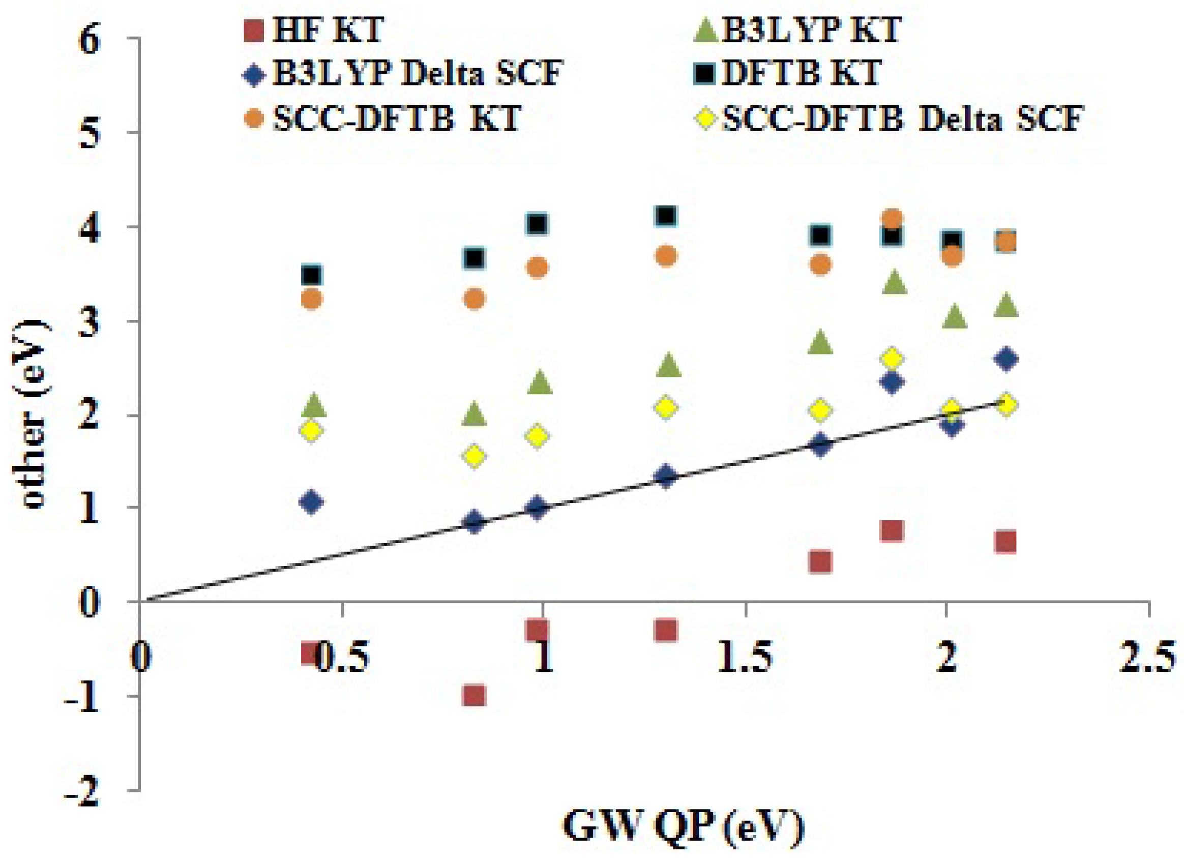
Figure 11 shows how the DFTB and other approximate methods compare to our $GW$ QP EA BDS. To get an idea of predictability, see Table 8. The HF KT EAs are expected to be an underestimate of the experimental values. Indeed, both relaxing the $(N+1)$-electron state and taking into account the greater correlation energy of the $(N+1)$-electron system compared to that of the N-electron system indicate that the HF KT EAs may be expected to be smaller than the true EAs. In this case, many of the HF KT EAs are negative and hence are unreliable unbound values. DFT KT EAs are expected to behave very differently, as the unoccupied DFT orbital energies may best be regarded as a first approximation on electronic excitation energies, which are typically smaller than EAs. This is seen in the overestimation of EAs by the DFTB KT and SCC-DFTB KT methods. As the B3LYP functional contains some admixture of HF exchange, it is normal that the B3LYP KT EAs lie somewhere in between the (SCC-)DFTB KT and HF KT methods. The ΔSCF method results in a dramatic improvement for EAs in both the SCC-DFTB and B3LYP cases, with particularly good absolute EAs being produced by the B3LYP ΔSCF method. Table 8 suggests that the main difference between the LDA, B3LYP and SCC-DFTB KT and ΔSCF values is more in the value of the intercept b than in a change in the slope m. This is consistent with the idea that the KT calculations contain a derivative discontinuity contribution not present in the ΔSCF calculations. As commented on earlier, this is not true for the original non-SCC DFTB method where the KT and ΔSCF calculations always give the same result. Furthermore, comparing Table 7 and Table 8, we see that the main difference between the IP and EA B3LYP KT and SCC-DFTB KT fits is also in the intercept b, rather than the slope m, also consistent with an important derivative discontinuity effect. Interestingly, the IP and EA B3LYP ΔSCF fits show only a small shift of the intercept b, while the IP and EA SCC-DFTB ΔSCF fits show a more distinct shift.

Figure 10. Inversion plot showing how fitting parameters obtained for the SCC-DFTB KT IPs and medium-sized molecules predict the GW QP IPs of medium-sized molecules and the experimental IPs of small molecules.

Figure 10. Inversion plot showing how fitting parameters obtained for the SCC-DFTB KT IPs and medium-sized molecules predict the GW QP IPs of medium-sized molecules and the experimental IPs of small molecules.

Figure 11. Correlation graph of data from Table 5 showing how the DFTB, SCC-DFTB and other methods (y-axis, eV) compare with $GW$ QP (x-axis, eV) EAs.

Figure 11. Correlation graph of data from Table 5 showing how the DFTB, SCC-DFTB and other methods (y-axis, eV) compare with $GW$ QP (x-axis, eV) EAs.

Table 8. Fitting data for first EAs of the medium-sized benchmark dataset (BDS) molecules: $y=mx+b$, where x is the $GW$ EA and y is another theoretical EA, both in eV. HF, Hartree–Fock; OVGF, outer valence Green’s function; LDA, local density approximation; DFTB, density-functional tight binding (without self-consistent charge); SCC-DFTB, self-consistent charge DFTB.

Method	m (Unitless)	b (eV)	$\Delta y$ (eV)	$\Delta x$ (eV)
Koopmans’ Theorem
HF ${}^a$	−0.817	1.772	0.181	0.222
HF ${}^b$	1.455	−1.695	0.860	0.591
HF ${}^c$	0.971	−1.289	0.344	0.354
OVGF ${}^d$	1.183	−0.777	0.475	0.402
OVGF e	0.948	−0.578	0.487	0.513
LDA	0.801	2.815	0.197	0.246
B3LYP	0.769	1.645	0.218	0.284
DFTB	0.151	3.672	0.195	1.298
SCC-DFTB	0.407	3.089	0.186	0.458
ΔSCF
HF ${}^a$	1.020	−0.833	0.460	0.451
LDA	0.917	1.107	0.303	0.331
B3LYP	0.926	0.330	0.317	0.342
DFTB	0.150	3.672	0.195	1.298
SCC-DFTB	0.340	1.552	0.252	0.740

${}^a$ HF/6-31G*//HF/6-31G*, ${}^b$ HF/6-31G//B3LYP/6-31G**, except for PCBM, which was calculated at the HF/STO-3G//B3LYP/6-31G** level. ${}^c$ HF/6-31G//B3LYP/6-31G**, excluding PCBM. ${}^d$ OVGF/6-31G//B3LYP/6-31G**, except for PCBM, which was calculated at the OVGF/STO-3G//B3LYP/6-31G** level. e OVGF/6-31G//B3LYP/6-31G**, excluding PCBM.

Table 8. Fitting data for first EAs of the medium-sized benchmark dataset (BDS) molecules: $y=mx+b$, where x is the $GW$ EA and y is another theoretical EA, both in eV. HF, Hartree–Fock; OVGF, outer valence Green’s function; LDA, local density approximation; DFTB, density-functional tight binding (without self-consistent charge); SCC-DFTB, self-consistent charge DFTB.

Method	m (Unitless)	b (eV)	$\Delta y$ (eV)	$\Delta x$ (eV)
Koopmans’ Theorem
HF ${}^a$	−0.817	1.772	0.181	0.222
HF ${}^b$	1.455	−1.695	0.860	0.591
HF ${}^c$	0.971	−1.289	0.344	0.354
OVGF ${}^d$	1.183	−0.777	0.475	0.402
OVGF e	0.948	−0.578	0.487	0.513
LDA	0.801	2.815	0.197	0.246
B3LYP	0.769	1.645	0.218	0.284
DFTB	0.151	3.672	0.195	1.298
SCC-DFTB	0.407	3.089	0.186	0.458
ΔSCF
HF ${}^a$	1.020	−0.833	0.460	0.451
LDA	0.917	1.107	0.303	0.331
B3LYP	0.926	0.330	0.317	0.342
DFTB	0.150	3.672	0.195	1.298
SCC-DFTB	0.340	1.552	0.252	0.740

${}^a$ HF/6-31G*//HF/6-31G*, ${}^b$ HF/6-31G//B3LYP/6-31G**, except for PCBM, which was calculated at the HF/STO-3G//B3LYP/6-31G** level. ${}^c$ HF/6-31G//B3LYP/6-31G**, excluding PCBM. ${}^d$ OVGF/6-31G//B3LYP/6-31G**, except for PCBM, which was calculated at the OVGF/STO-3G//B3LYP/6-31G** level. e OVGF/6-31G//B3LYP/6-31G**, excluding PCBM.

6. Conclusions

As emphasized, for example, by the Shockley diode model presented in the Appendix and perhaps even better by the Shockley-like model developed in [5] specifically for organic solar cells, it is important to be able to understand the underlying phenomenology of organic photovoltaics at the atomistic level. However, these are complex systems that can benefit from both molecular and solid-state theory and that ultimately are likely to require hybrid approaches, which are somewhere between what is now standard for molecules and what is now standard for inorganic solids. It is a problem, in fact, at the “nanoscale interface” between these two ideological paradigms, which is likely to require the modeling the electronic structure and dynamics of ensembles of objects on the order of 1–100 nm in size. As this is beyond the reach of most first principles methods, we have decided to adopt the semi-empirical DFTB approach as a way to try to extend first principles accuracy to larger systems. Naturally, this also requires us to accept some loss of accuracy whose magnitude we have tried to evaluate for IPs and EAs of small molecules and of medium-sized molecules of interest for organic electronics.

This paper has presented a test of the accuracy of DFTB and especially of third-order SCC-DFTB. It has been possible to determine this for larger molecules than is usually the case because of our access to the recently-developed $GW$ methodology, which itself has been checked against available experimental values. The final result is that DFTB3 with the 3ob parameter set is found to give the first IPs with an accuracy of ±0.489 ev/±0.326 eV with the SCC-DFTB ΔSCF/KT approaches. To judge from Figure 10, lower IPs may also be determined with a similar accuracy using the SCC-DFTB KT method. The first EAs are found to be accurate to ±0.740 eV/±0.458 eV with the SCC-DFTB ΔSCF/KT approaches. We find this quite encouraging and expect that one should still be able to answer quite a few well-posed questions in organic electronics with this level of accuracy. There is a caveat, however: the reader should keep in mind that results will change if a different implementation of DFTB and/or another parameter set are used.

A perhaps more important observation is that, while it is possible to optimize a semi-empirical method explicitly for IPs and EAs, the parameters in the DFTB method have not been optimized with this end in mind, but rather with the idea of being a well-balanced approximation to DFT. Thus, we repeatedly find that DFTB is behaving like DFT rather than, say, a correlated HF-based ab initio method. Moreover, though the SCC-DFTB formalism differs significantly in details from the self-consistent solution of the DFT equations, we do find that (much like in DFT) the best way to calculate IPs and EAs is to use the ΔSCF method with SCC-DFTB. However, much like in regular DFT calculations, SCC-DFTB KT IPs are also found to be a reasonable way to estimate the first several IPs simultaneously and, hence, to obtain the molecular analogue of band spectra. Such a similarity with DFT, together with the capacity to go to larger and more complex systems, makes DFTB particularly attractive to us as we wish to go well beyond merely studying IPs and EAs to using DFTB to study the details of photochemical processes at the donor-acceptor interface in organic solar cells, as all indications point to the details of polaron pair dissociation as being a key determining step to organic photocell performance [5]. Of course, where possible, we will continue to check our DFTB results against experiment and against good first-principles computational methods as we go along.