
Scatter Search Applied to the Inference of a Development Gene Network


1
Computational Science Lab, University of Amsterdam, Science Park 904, 1098XH Amsterdam, The Netherlands
2
EMBL/CRG Systems Biology Research Unit, Centre for Genomic Regulation (CRG), The Barcelona Institute of Science and Technology, 08003 Barcelona, Spain
3
Universitat Pompeu Fabra (UPF), 08003 Barcelona, Spain
4
Centre for Interdisciplinary Research in Biology, College de France, CNRS, INSERM, PSL Research University, 75231 Paris, France
*
Author to whom correspondence should be addressed.
Computation 2017, 5(2), 22; https://0-doi-org.brum.beds.ac.uk/10.3390/computation5020022
Submission received: 10 March 2017
/
Revised: 19 April 2017
/
Accepted: 28 April 2017
/
Published: 4 May 2017
(This article belongs to the Special Issue Multiscale and Hybrid Modeling of the Living Systems)
Abstract
:Efficient network inference is one of the challenges of current-day biology. Its application to the study of development has seen noteworthy success, yet a multicellular context, tissue growth, and cellular rearrangements impose additional computational costs and prohibit a wide application of current methods. Therefore, reducing computational cost and providing quick feedback at intermediate stages are desirable features for network inference. Here we propose a hybrid approach composed of two stages: exploration with scatter search and exploitation of intermediate solutions with low temperature simulated annealing. We test the approach on the well-understood process of early body plan development in flies, focusing on the gap gene network. We compare the hybrid approach to simulated annealing, a method of network inference with a proven track record. We find that scatter search performs well at exploring parameter space and that low temperature simulated annealing refines the intermediate results into excellent model fits. From this we conclude that for poorly-studied developmental systems, scatter search is a valuable tool for exploration and accelerates the elucidation of gene regulatory networks.
1. Introduction
One of the big challenges in current-day biology is efficient network inference (also known as reverse engineering) [1]. It is the so-called inverse problem of deducing which genes interact and how strong each interaction is on the basis of the network’s observed output, its expression dynamics. By tackling this challenge successfully, we gain insight in the internal dynamics of a regulatory network. In turn, this understanding aides the explanation of existing experimental results and helps us formulate hypotheses and new experiments to further probe the biological system under study. While on the experimental side obtaining the required data is often laborious and difficult, here we take the data as a given and focus on the computational side of network inference.
With the currently available computational power of a single workstation, network inference in a unicellular context is a successful endeavour, such as for yeast genetic and metabolic networks [2,3], and for the optimization of specific bio-molecules in bacteria [4] and in mammalian cell lines [5,6,7]. Moreover, the study of such systems is supported by software tools [8], formal languages for model description that enhance sharing and re-use [9,10], and crowd-sourcing efforts (e.g., DREAM Challenges [11]).
In developmental biology, network inference is used to compare and better understand how organisms create spatial and temporal patterns to grow and shape themselves. Networks of interacting genes are key players in these dynamical processes. Well-known examples are body plan formation in insects [12,13,14,15,16] and sea-anemones [17], limb development [18,19], and vulva cell differentiation [20]. The multicellular context, however, means an additional computational challenge. In the tissue that is being patterned, each cell has a gene network and (in general) communicates with other cells, thus creating a large system of coupled gene networks. This means that as we move from describing a single cell to a multicellular setting, the number of variables of the system increases dramatically (though the number of parameters remains rather similar to the single cell case). As a result, to do a rigorous, automated, fitting of model parameters, increased system size makes calculations computationally demanding. In fact, one is often restricted to high-performance computing (HPC) facilities.
Regardless of whether one studies single cells or patterning tissues, when one is deriving a network from data, swift feedback from the inference algorithm is highly desirable. The effort of building a model usually requires several iterations of inferring the regulatory network to arrive at a satisfactory solution. Hence a fast algorithm is not only convenient, it also allows for a better study of the network through alternative scenarios and systematic assessment of the influence of parameters on the system. Each iteration of inference provides information that may be used to adjust the algorithm and to analyse the solutions that have been produced. It follows that an important feature is the computational cost of an algorithm used for network inference.
Here, we address the issue of computational cost and swift feedback in the context of a developmental regulatory network—the gap gene system, introduced below—responsible for early body plan formation in insects. We introduce a hybrid, two-stage optimization approach to infer the network. The idea behind the two-stage approach is to first explore parameter space with scatter search. Scatter search is a population-based approach, that has been building a solid reputation for solving combinatorial and nonlinear optimization problems [21,22]. Indeed, a solver based on scatter search was found to be the best stochastic solver tackling 1000 global optimization problems and outperformed other methods in black-box challenges [23]. In the last decade, scatter search has been adapted for nonlinear dynamic biological systems (and continues to be further developed, see Discussion) [21,22]. Its biggest advantage is that it is a computationally light method and thus provides rapid feedback on the structure of the network.
Once after several rounds of exploration a set of promising solutions is established, in a second stage low temperature simulated annealing is used to refine them. We evaluate the strengths and weaknesses of the hybrid approach against ‘normal’ simulated annealing. We use a parallel implementation of simulated annealing, pLSA, that over the last two decades has been our algorithm of choice as it finds excellent solutions that faithfully reproduce expression data and spatial patterns [12,14,24]. While we restrict ourselves here to a comparison of scatter search with simulated annealing, we note that also evolutionary optimization algorithms have been used to tackle the challenge of insect body plan formation [25,26,27].
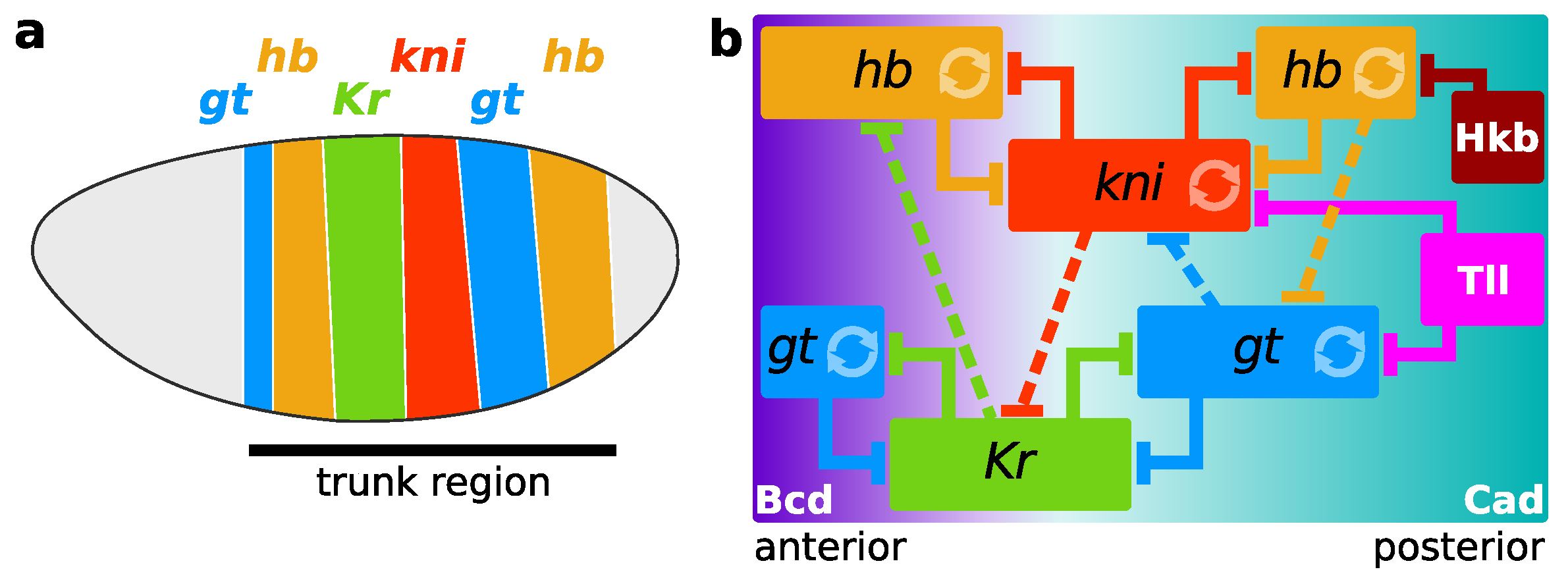
As a benchmark system, we use the gap gene network of the fruit fly Drosophila melanogaster (Figure 1a). It is the regulatory network that lays down the initial body plan of the fly during the blastoderm stage of early development, before the onset of gastrulation (Figure 1b). It consists of three maternal gradients, namely Bicoid (Bcd), Caudal (Cad), and Hunchback (Hb), that are interpreted by four trunk gap genes, hb, Krüppel (Kr), giant (gt), and knirps (kni)). As a result, the trunk gap genes form a series of broad stripes along the antero-posterior (A–P) axis. At the posterior end, the terminal gap genes tailless (tll) and huckebein (hkb) regulate the trunk gap genes. The gap gene system is one of the best understood developmental networks from both an experimental and modelling point of view, and thus a good benchmark case [28].
In comparison to other developmental systems, the Drosophila embryo has some key advantages. The early embryo is a syncytium (multi-nucleated cell), so we may ignore intercellular signalling. There is no tissue growth or rearrangement during the blastoderm stage. Moreover, patterning by gap genes in the trunk region occurs only along the A–P axis, and is decoupled from other patterning processes, such as those along the dorsal-ventral axis. These properties allow us to simplify the system to a one-dimensional array of (dividing) nuclei along the A–P axis. Indeed, due to its modelling-friendly properties, the gap gene system has been studied with a variety of models and methods [29,30,31,32,33,34,35].
We employ the gene circuit approach to model the Drosophila embryo [12,13,14,24,36,37,38]. A gene circuit is a dynamical hybrid model of coupled ordinary differential equations (ODEs). An embryo is represented as a row of nuclei that divide over time, where each nucleus has an identical instance of the gap gene regulatory network. The ODEs encode the network through regulated synthesis of gene products (mRNA or protein), Fickian gene product diffusion between neighbouring nuclei, and linear decay of the gene product. For D. melanogaster, the system has 41 parameters and fitting these may be classified as an optimization task of medium size. Originally, gene circuits were developed to fit quantitative protein expression data [12,13,38]. The acquisition and processing of such data are a laborious and time-consuming effort, and are not easily applied to nonmodel organisms. Recent studies, however, have shown the wider applicability of the gene circuit approach by developing protocols based on mRNA expression data, not only in D. melanogaster [14], but also in nonmodel organisms [15,16]. Moreover, gene circuits allow for simultaneous inference of which interactions are present, whether they are activating/inhibiting, and the strength of these interactions. It sets the gene circuit approach apart from other modelling efforts, where the topology is predefined and the task is to establish which interaction strengths fit the data best (known as parameter estimation). Together, these properties make fitting gene circuits an ideal test case for scatter search. It is a challenging task, it has an immediate practical relevance in systems biology, and has been shown to be successful for the inference of unknown gene regulatory networks.
We show that a hybrid, two-stage approach to network inference problems in developmental biology delivers equally good results as simulated annealing, our current default method. We find that scatter search efficiently and effectively explores the parameter space, and that low temperature simulated annealing turns good solutions into excellent ones. These results suggest that it is a promising method for inferring unknown networks, such as the one laying down the body plan of the sea anemone Nematostella vectensis [17,39,40], where multiple rounds of exploration are likely necessary. Moreover, given the additional computational costs for simulating systems in which morphogenetic processes play an important role (e.g., 2D and 3D models including cell migration, tissue rearrangements, growth, cell death) a light explorative method will be a prerequisite for success.
2. Materials and Methods
2.1. Scatter Search Method
Scatter search is a global optimization algorithm related to the family of evolutionary algorithms [41]. As do evolutionary algorithms, the method maintains a population of solutions and combines these solutions to obtain new ones. However, the underlying search strategy is different (see [21,22] for an in depth discussion). We implemented a sequential version of scatter search, closely following a set of guidelines developed for applications in biology [21,22].
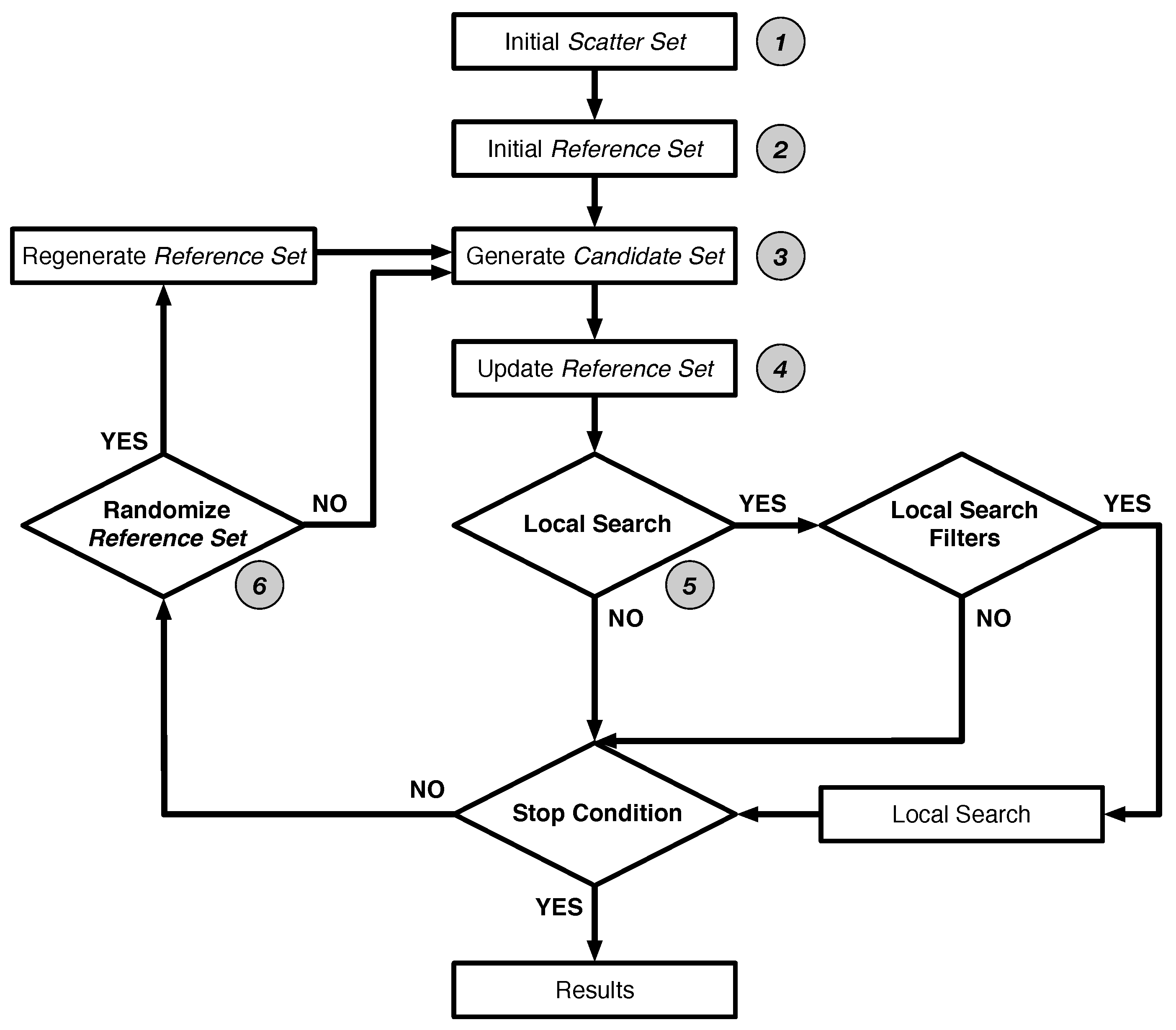
The algorithm operates as follows (Figure 2). In an initial phase, (1) scatter search generates a large set of diverse solutions, named the Scatter Set. The goal is to have an initial set of solutions that reasonably covers the parameter search space. To this end, the diversity of solutions is maximised by subdividing parameter space into bins and uniformly sampling parameter values across these bins. Then (2) the algorithm creates the main population of solutions named the Reference Set. A set of solutions is selected from the Scatter Set on the basis of their quality and diversity: half of the reference set contains the best solutions, i.e., elite solutions, and the other half consists of diverse solutions (in terms of parameter values). This dual use of the Reference Set is maintained during the optimization phase.
After initialization, scatter search iterates the following steps until a stop condition is satisfied. In our case, the algorithm performs a fixed number of iterations. In every iteration, (3) the algorithm produces a set of candidate solutions, Candidate Set, by creating linear combinations of every pair of solutions in Reference Set. Next, (4) the worst solutions in Reference Set are replaced by better candidates, taking into account quality and diversity of the candidates. Before starting the next iteration, (5) the algorithm may apply a local search on the members of Reference Set to accelerate convergence. By default the Nelder-Mead simplex algorithm is used, additionally we used Stochastic Hill climbing. In our implementation, the user decides beforehand if local search is enabled, and under which conditions it is applied (Local Search Filters in Figure 2) . These filters help to avoid time-consuming evaluations of solutions. We provide one, filter_different_enough, that checks if a solution has sufficiently distinct parameters from other members of Reference Set. This avoids regions of search space that are already being explored. The second filter, filter_good_enough, only allows good individuals, as local search is most effective if the starting solution is good [42,43]. Finally, (6) occasionally no candidates replace the current members of Reference Set. In such a case, we consider the algorithm to be stuck in a specific region of parameter space. Scatter search overcomes such an impasse by randomizing a part of Reference Set using a newly generated Scatter Set.
Scatter search is implemented in C and requires two third-party libraries: SUNDIALS (http://computation.llnl.gov/projects/sundials) and GSL (https://www.gnu.org/software/gsl) [44]. Source code is available on GitHub at https://github.com/amirmasoudabdol/flyOpt. We compiled the code with GCC 4.7.2 (https://gcc.gnu.org)) using the -O2 optimization flag. We have run scatter search simulations on the Lisa system of SURFsara (https://userinfo.surfsara.nl/systems/lisa) using search parameters as listed in Table 1. We saturated single nodes (Intel Xeon CPUs at 2.6 GHz, 16 cores) with the maximum of 16 runs to suppress hardware parallelism. We note that these tests were run on a HPC facility simply for convenience. The software does not use any parallel computation features and the hardware of current-day workstations is often comparable to that of the Lisa system.
2.2. Parallel Simulated Annealing
Simulated annealing (SA) is a probabilistic global optimization algorithm, originally formulated in the 1980s [45]. It operates in analogy to metallurgic annealing, the process of slowly cooling metal in order to reach a low-energy equilibrium state. In simulated annealing the energy level is the cost of a solution, and the notion of cooling is implemented as slowly reducing the probability of accepting a new candidate with a worse cost.
The basic structure of SA has three components. First of all, it requires a so-called ‘move’ function that creates from the current solution a neighbouring ‘mutant’ solution. Second, there is a policy to accept or reject the new solution. The cost of the old and new candidates and the current temperature are taken into account to make the decision. Third, an annealing schedule determines how to lower the temperature as the algorithms progresses. The key parameter is the temperature. It determines the acceptance rate of new solutions with worse cost than the current one: the lower the temperature, the lower the probability of acceptance. Thus, starting with a high temperature, SA initially samples across the entire parameter space. As the algorithm moves from one solution to another, the annealing schedule lowers the temperature and over many ‘moves’ the algorithm biases progressively towards better solutions. The (occasional) acceptance of worse solutions ensures that it escapes local optima.
The strength of SA is that it works very well for a wide variety of (biological) optimization problems. Moreover, given certain requirements, it is mathematically proven to find the global minimum. However, its weakness is a large computational footprint. Therefore, we use parallel Lam Simulated Annealing (pLSA), developed by [46]. It is a parallel implementation of SA with the adaptive annealing schedule of [47,48]. The approach is based on the observation that the acceptance policy maintains a Boltzmann distribution of energies. By combining statistics from all processing nodes, and a mixing of node states at given intervals, such a Boltzmann distribution is ensured also in the parallel case.
pLSA is implemented in C and uses MPI, SUNDIALS, and GSL. pLSA is run (with settings given in Table 2) at the Barcelona Supercomputing Center, using Mare Nostrum 3 computing facilities. It is compiled with the Intel compiler v13.0.1 using the -O3 optimization flag and Intel MPI library. A single pLSA run is executed on 64 cores. Nodes have Intel Sandybridge CPUs (8 cores) at 2.6 GHz, with at least 2 GB of working memory per core.
2.3. Gene Circuits, Simulation, and Analysis
The gap gene regulatory network is modelled as a gene circuit [24], described in detail elsewhere [13,14]. In short, we model the trunk region of the D. melanogaster embryo as a linear array of nuclei. The trunk region is defined for mRNA expression data from 35% to 87% A–P position, and for protein data 35–92% (0% is the anterior pole). In each nucleus, there is continuous regulation and expression of gap genes, while over time the number of nuclei doubles through discrete mitotic division. Gene regulation and expression over time t is governed by coupled ordinary differential equations (ODEs):
with , gene expression product (mRNA or protein, depending on the data) at nucleus i of gap gene (G is defined below). Parameters , and are production, diffusion, and decay rates. Diffusion depends on the number of previous divisions n. Eukaryotic gene regulation is phenomenologically modelled as a sigmoid response curve with a summation over genetic interactions :
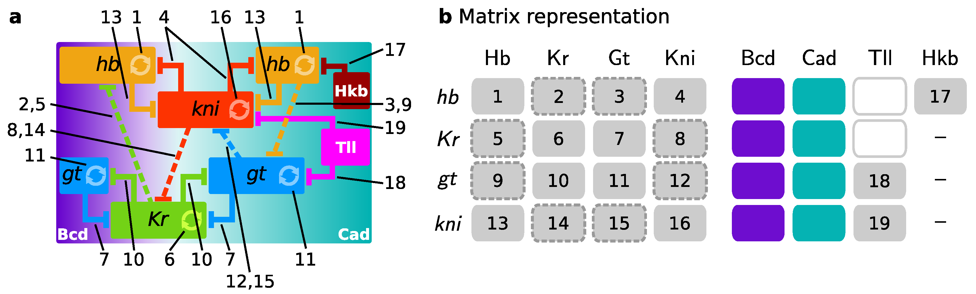
with trunk gap genes and external inputs . Parameter matrices W and E define genetic interactions between trunk gap genes and external inputs on trunk gap genes, respectively. Each parameter (and ) represents the effect of regulator b (m), on gap gene a. We interpret that the regulator has an activating role if () is positive (); an inhibitory role if negative (); and there is no interaction if the value is near zero (). The interpretation is visualized as a network diagram (Figure 3a) or as a genetic interaction matrix (Figure 3b). Parameter represents background maternal factors and is fixed at for all trunk gap genes. In total, a gene circuit has 41 parameters.
As mentioned in the Introduction, D. melanogaster gap genes are expressed during late blastoderm, in mitotic cycle C13 and C14A. Gene circuit equations are solved from the start of C13 (t = 0 min), when gap gene expression becomes detectable, until the onset of gastrulation at the end of C14A (t = 71.1 min). Mitosis occurs during t = 16–21 min, during which gene product synthesis is set to zero. Gene circuits have 108 ODEs in C13, and 212 ODEs in C14A. Regardless of the optimization algorithm, gene circuits are numerically integrated using two solvers. If circuits are inferred from mRNA expression data, an implicit multi-step method is used (CVODE, Sundails library) [44]. In case protein expression data are used, we employ a Runge-Kutta Cash-Karp adaptive step-size method [12].
The cost of a gene circuit is the sum of residuals when comparing the circuit output with experimental data. It is minimized by the optimization algorithms, and we formulate it as a weighted least squares [13,14]:
with G the set of trunk gap genes, T the set of time points for which we have data (C13, C14A: T1–T8), the number of nuclei after n mitotic cycles, weights, and the mRNA or protein expression level of gap gene a in nucleus i at time point t. For interpretation, we may also express the cost as a Root Mean Square (RMS), which ignores the weights v and is a normalization with respect to the total number of data points ( and ).
After optimization, the resulting solutions are judged on RMS, numerical stability, and visual inspection of model output, as described in detail elsewhere [13,14]. Analysis and plotting is performed using the previously developed SuperFIT package (https://app.assembla.com/spaces/superfit/subversion/source) [16].
3. Results
3.1. Scatter Search Efficiently Explores Parameter Space
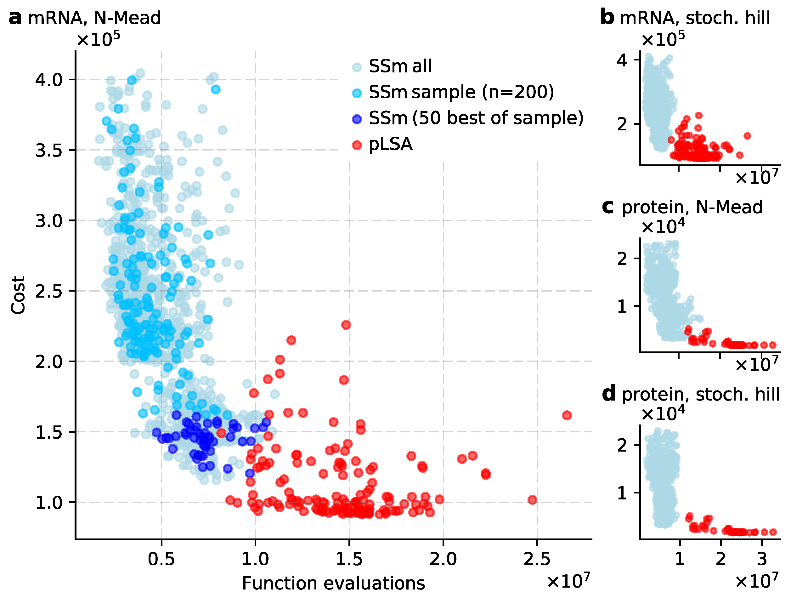
Our first goal was to broadly characterize the performance of scatter search in the context of inferring the network of gap gene interactions in D. melanogaster. We generated a large set of solutions by starting 1000 scatter search simulations and taking the final best solution from each of them. We focussed on the networks derived from D. melanogaster mRNA expression data (Figure 4a) [14], while we obtained similar results for protein expression data (Figure 4c,d) [13]. The cost of mRNA-derived solutions, as defined in Equation (3), ranged from to , with an average of (and median ). As scatter search only applied the local search method, if a solution’s cost is below , there is a lack of solutions just below this cost (Figure 4a, ‘Local search score’ in Table 1). From these 1000 solutions, we sampled 200 for further study and analysis (Figure 4, blue dots).
Next, we used pLSA to generate a second set of solutions by fitting 150 gene circuits to mRNA expression data. We made three noteworthy observations in the comparison of both methods (Figure 4). First, the average scatter search run executes substantially fewer function evaluations than an average pLSA run ( against ). Second, we defined good and excellent solutions to have, respectively, a cost and . With this categorization, scatter search finds many good solutions, but not any excellent ones. Instead, pLSA does find excellent solutions that are suitable for in-depth biological analysis. Third, the relation between cost and function evaluations suggests there is a Pareto front, where a certain minimal number of evaluations are necessary to reach a given cost (Figure 4a). Intuitively it makes sense, as good and excellent solutions are rare and it requires computational effort to find them. We place a cautionary note, though, as we observed that the shape of the (potential) Pareto front depends on the local search method used in scatter search and the type of expression data (mRNA/protein). If we use Stochastic Hill climbing or protein data, the front changes shape and the trade-off between cost and function evaluations is less visible (Figure 4b–d).
Thus, despite the population-based approach, scatter search is a computationally light search method (also noted by [21]). Moreover, the strength of scatter search is that it efficiently surveys parameter space and identifies promising areas that can be further explored (i.e., analysing the good solutions). Its weakness, however, is that it does not find as excellent solutions as pLSA does.
3.2. Exploiting the Exploration Done by Scatter Search
Even if scatter search solutions do not reproduce expression data at the desired level of biological correctness, they provide a first view on the structure of the gene network. As argued in the Introduction, such a quick first view is a valuable source of information, especially in the case of unknown gene networks or computationally expensive models. The gap gene network of D. melanogaster is a good test case, as we know its structure well. We asked what biological insight is already contained in the 50 best solutions inferred by scatter search.
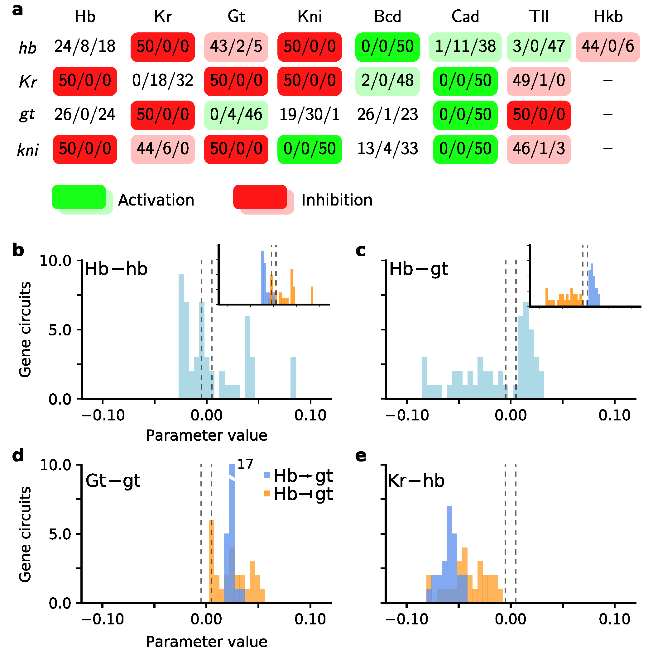
We created a first view of the gap gene network by categorizing the genetic interactions in the 50 best gene circuits (Figure 5a). Almost half (14/29) of the interactions show full consensus, while 10/29 show a clear trend towards activation or inhibition. In previous work, the genetic interactions were grouped in five mechanisms [12,13,14]. Focussing on the consensus interactions, we immediately observed the two major mechanisms: alternating cushions and maternal activation. The former is comprised of two pairs of strongly repressing gap genes, namely hb/kni and gt/Kr, while the latter requires that Bcd and Cad activate the gap genes. We see that Bcd is essential for hb activation, while Cad is crucial for gt and kni. Kr is thought to be mainly under control of Bcd [28] and we find that with two exceptions it is the case. Experiments, however, show Kr expression in embryos without Bcd, which may be explained by a redundant role for Cad [28]. Indeed we have consensus for activation by Cad (Figure 5a).
The third mechanism is the shifting of posterior gap gene domains in an anterior direction, i.e., towards the head region. These shifts require an asymmetric regulation between neighbouring expression domains, which are only partially observed here, namely for Kr/kni. In Drosophila, the hb/Kr boundary is an exception as it does not display anterior shifts. Instead, the two gap genes inhibit each other strongly and establish a boundary with a fixed position along the A–P axis. Indeed, we observed a consensus for mutual inhibition. The fourth mechanism is self-activation of the gap genes, which is clear for gt and kni at this stage of network inference. Finally, we observe that Tll represses Kr, gt and kni, which ensures they are not expressed in the posterior terminal end.
We obtained a more detailed view by inspecting the distribution of parameters for specific interactions. We focused on the regulation of hb and gt by Hb, as scatter search predicts multiple, qualitatively different outcomes for these interactions. First, hb self-regulation tends towards inhibition (compare Figure 5a,b). Yet the parameter distribution gives us the insight that only a small amount of inhibition is tolerated, while neutral behaviour and especially activation are accepted for a wide range of values. Second, for the regulation of gt by Hb (Figure 5c), we noticed that the regulatory effect of Hb on gt was split along either inhibition or activation. We asked if the two alternative regulatory effects on gt correlate with distinct sets of gene circuits. We compared the set of gene circuits with Hb inhibiting gt to the circuits with Hb activating gt, and observed two major differences. First, and most importantly, circuits with inhibition of gt show a wider range of values for several interactions. Examples are gt self regulation (Figure 5d) and Kr regulation of hb (Figure 5e). Second, inhibition of gt by Hb correlates clearly with hb self-activation. Activation of gt by Hb, on the other hand, is accompanied by hb self-inhibition (Figure 5b, inset). Interestingly, the observed correlations between parameter distributions may be associated to canalizing properties of the gap gene network to position the anterior hb boundary at ∼50% A–P position [49,50]. A dynamical systems analysis of this hb boundary showed a nonlinear dependence on Bcd, gt, and Kr during the late blastoderm stage [50], which may explain scatter search finding multiple regulatory solutions. Yet a complementary explanation that cannot be ruled out, is that as hb and gt expression domains appear at the edges of the modelled region, additional regulatory factors could be missing [49].
We hesitate interpreting the more subtle differences between the two sets of circuits. In this test case of the D. melanogaster gap gene network, it is straightforward to link our observations to our knowledge of the wildtype network structure. However, if a network is unknown, interpreting subtle cues easily leads to errors where model artefacts are taken to have a biological meaning. Nevertheless, there is a clear potential for inspecting intermediate results and drawing conclusions from them that may guide a next iteration of network inference.
3.3. Low Temperature Simulated Annealing Refines Good Solutions into Excellent Ones
After exploring the gene circuits proposed by scatter search, in the second stage we set out to refine them with the goal of obtaining solutions that are as excellent as the ones generated by simulated annealing. As the scatter search circuits perform well, we decided to take them as starting points for optimization with low temperature simulated annealing. By skipping the initial moves of simulated annealing and beginning with a relatively low temperature, we avoid the early randomizing behaviour of this search method. Instead, the algorithm is likely to make only modest changes and is likely to preserve the structure of the network. In effect, this mode of simulated annealing is focussed on a particular area of parameter space.
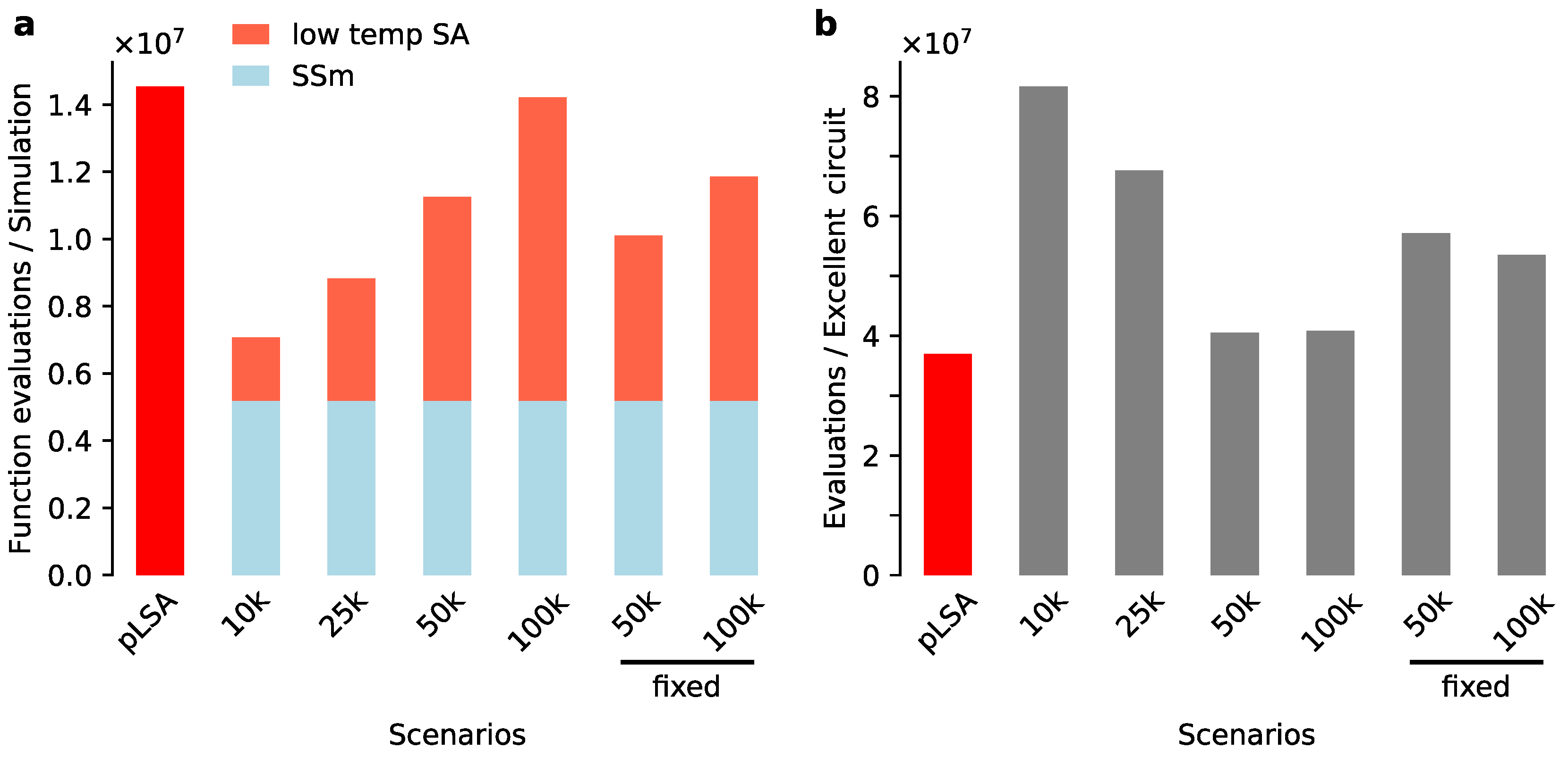
First we filtered the 200 solutions by removing all with a cost >. We continued with 143 remaining solutions. To assess the effect of different starting temperatures, we surveyed four scenarios with a range from T to (Figure 6). Moreover, for T = 50 k and 100 k, we tested how simulated annealing performed under a restriction of its search space. For each consensus interaction as inferred in the first stage (Figure 5a) the range of allowed parameter values was limited by the sign of the interaction. For instance, scatter search indicated that Kni represses hb, and therefore, we limited this interaction to negative values only. After fitting gene circuits, the results of non-fixed and fixed low temperature SA were compared to each other and to the standard use of pLSA by computational performance (number of function evaluations) and quality of the inferred networks.
With respect to computational performance, we found that the starting temperature has a strong influence on the performance of simulated annealing. At first sight the two-stage approach appeared more efficient than pLSA (Figure 6a). With the exception of T = 100k (non-fixed), the two-stage approach required fewer function evaluations than pLSA to generate a set of excellent gene circuits. That was anticipated, as a lower starting temperature means that simulated annealing accepts worse solutions with a lower probability than is the case for a normal optimization run with pLSA. Thus convergence is more rapid. As expected, the restricted search space of fixed scenarios reduced the number of function evaluations in comparison to the corresponding non-fixed scenarios. Yet, the reduction did not lead to an increase in efficiency of finding excellent solutions (Figure 6b). We realized that restricting search space excludes many of the 143 gene circuits as valid starting points for SA, as they have one or more parameters in a forbidden area of search space. This indicates that in the non-fixed scenarios, low temperature SA still changed the topology of ‘bad’ networks and that this is a beneficial feature.
In general, compared to pLSA, the number of function evaluations per excellent solution is equal or higher for the hybrid, two-stage approach (Figure 6b). That would argue against our two-stage approach. However, if several iterations are needed either for the first exploratory stage or the later refining one, the hybrid approach will be less computationally costly than doing several rounds of ‘full’ pLSA runs. Especially, the scenario T = 50 k (non-fixed) will rival the performance of pLSA.
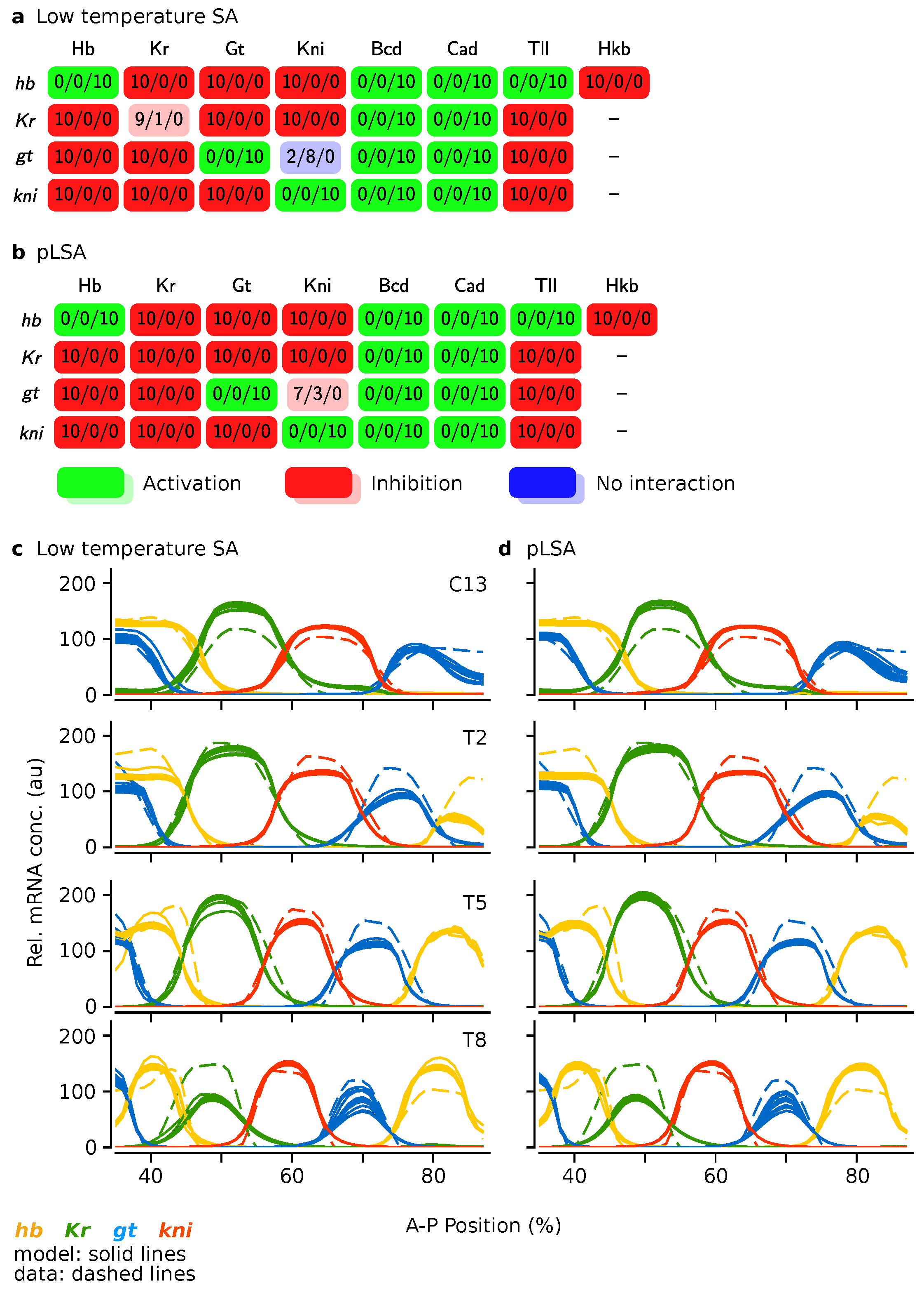
We continued by comparing the best solutions of both approaches. We selected the 10 circuits with lowest RMS, and generated genetic interaction matrices (Figure 7a,b) and gene expression profiles (Figure 7c,d). We found that hybrid runs from intermediate temperatures have the least number of defects (visual inspection, data not shown for T = 25 k). Most importantly, two-stage solutions are just as good as the ones generated by pLSA, both in terms of interaction matrix and expression profile.
4. Discussion
For network inference of spatiotemporal patterning, especially in flies, we traditionally used parallel Lam simulated annealing. It is a computationally costly method, but produces excellent results across different species of flies [12,13,14,15,16]. Here we reported on an alternative, hybrid approach consisting of two stages: first we applied scatter search to develop an initial understanding of the network, followed by low temperature SA to refine good solutions into excellent ones. The alternative approach delivered equally good results in terms of genetic interactions and gene expression profiles. However, the total cost of both stages of network inference is slightly higher than for pLSA. Thus we recommend the alternative approach if repeated rounds of exploration of parameter space and tweaking of the algorithms are necessary.
Considering only few developmental gene regulatory networks are understood in-depth, most (future) applications of network inference will involve inferring an unknown network. In such cases, a 5 to 10 iterations are usually needed to tweak the algorithm, test alternatives, and get excellent solutions. Here the advantage of an initial exploration with scatter search is clear: the intermediate information that one can extract from good solutions is valuable and can be used to guide—or reduce the number of—subsequent iterations of network inference.
We point out that interpreting intermediate solutions has to be done with caution, as some of the findings may be misleading. Our test case of the gap gene network showed that scatter search generated at least two alternative network structures. While we know that one of them is unsupported by current experimental evidence, for an unknown network this information may not be available. From a more general perspective, it shows where the optimization algorithms struggles to find a unique solution. That may not be a satisfying result at first sight, yet it indicates a lack of knowledge and suggests specific experiments to improve our understanding of the system.
For a hybrid approach, the combination of scatter search and low temperature simulated annealing is not the only viable option. As was suggested in [26], (parallel) genetic algorithms are known to be good exploratory search methods as well. Moreover, with respect to our implementation of scatter search, recently a more advanced version of scatter search has become available, called saCeSS (self-adaptive cooperative enhanced scatter search) [51]. It uses multiple instances of scatter search set at different levels of exploration and exploitation, multiple local search methods, and utilizes the small-scale parallelism of current-day workstations. One expects saCeSS to perform better than our version of scatter search. In this sense, we have presented a worst-case performance scenario in this work. Also parallel LSA is still being improved. An asynchronous version has been released and it will be interesting to check its performance in the context of network inference [52].
Summarizing, for the inference of unknown networks scatter search is a valuable exploratory tool. It has light computational demands and delivers good solutions from which relevant information can be extracted. In a two-stage setting with simulated annealing, we expect it to be particularly effective in reducing the computational cost of network inference.
Acknowledgments
We thank Johannes Jaeger for critical feedback and scientific advice. We thankfully acknowledge the computer resources, technical expertise and assistance provided by the Barcelona Supercomputing Center, which is part of the Red Española de Supercomputación. We thank SURFsara (www.surfsara.nl) for the support in using the Lisa Compute Cluster. The Centre for Genomic Regulation (CRG) acknowledges support from the Spanish Ministry of Economy and Competitiveness, ‘Centro de Excelencia Severo Ochoa 2013-2017’, SEV-2012-0208. AC kindly acknowledges Fondation Bettencourt Schueller.
Author Contributions
A.M.A., J.A.K., and A.C. conceived and designed the experiments; A.M.A., D.C.-S., and A.C. performed the experiments; A.M.A. and A.C. analysed the data; A.M.A., D.C.-S., and A.C. contributed software and analysis tools; A.C. and A.M.A. wrote the paper with contributions of J.A.K.
Conflicts of Interest
The authors declare no conflict of interest.
References
- Villaverde, A.F.; Banga, J.R. Reverse engineering and identification in systems biology: Strategies, perspectives and challenges. J. R. Soc. Interface 2013, 11, 20130505. [Google Scholar] [CrossRef] [PubMed]
- Heavner, B.D.; Smallbone, K.; Price, N.D.; Walker, L.P. Version 6 of the consensus yeast metabolic network refines biochemical coverage and improves model performance. Database 2013, 2013, bat059. [Google Scholar] [CrossRef] [PubMed]
- Borodina, I.; Nielsen, J. Advances in metabolic engineering of yeast Saccharomyces cerevisiae for production of chemicals. Biotechnol. J. 2014, 9, 609–620. [Google Scholar] [CrossRef] [PubMed]
- Costa, R.S.; Hartmann, A.; Vinga, S. Kinetic modeling of cell metabolism for microbial production. J. Biotechnol. 2016, 219, 126–141. [Google Scholar] [CrossRef] [PubMed]
- Selvarasu, S.; Ho, Y.S.; Chong, W.P.K.; Wong, N.S.C.; Yusufi, F.N.K.; Lee, Y.Y.; Yap, M.G.S.; Lee, D.Y. Combined in silico modeling and metabolomics analysis to characterize fed-batch CHO cell culture. Biotechnol. Bioeng. 2012, 109, 1415–1429. [Google Scholar] [CrossRef] [PubMed]
- Saraiva, I.; Vande Wouwer, A.; Hantson, A.L. Parameter identification of a dynamic model of CHO cell cultures: An experimental case study. Bioprocess Biosyst. Eng. 2015, 38, 2231–2248. [Google Scholar] [CrossRef] [PubMed]
- López-Meza, J.; Araíz-Hernández, D.; Carrillo-Cocom, L.M.; López-Pacheco, F.; Rocha-Pizaña, M.D.R.; Alvarez, M.M. Using simple models to describe the kinetics of growth, glucose consumption, and monoclonal antibody formation in naive and infliximab producer CHO cells. Cytotechnology 2016, 68, 1287–1300. [Google Scholar] [CrossRef] [PubMed]
- Hoops, S.; Sahle, S.; Gauges, R.; Lee, C.; Pahle, J.; Simus, N.; Singhal, M.; Xu, L.; Mendes, P.; Kummer, U. COPASI—A COmplex PAthway SImulator. Bioinformatics 2006, 22, 3067–3074. [Google Scholar] [CrossRef] [PubMed]
- Hucka, M.; Finney, A.; Sauro, H.M.; Bolouri, H.; Doyle, J.C.; Kitano, H.; Arkin, A.P.; Bornstein, B.J.; Bray, D.; Cornish-Bowden, A.; et al. The systems biology markup language (SBML): A medium for representation and exchange of biochemical network models. Bioinformatics 2003, 19, 524–531. [Google Scholar] [CrossRef] [PubMed]
- Miller, A.K.; Marsh, J.; Reeve, A.; Garny, A.; Britten, R.; Halstead, M.; Cooper, J.; Nickerson, D.P.; Nielsen, P.F. An overview of the CellML API and its implementation. BMC Bioinform. 2010, 11, 178. [Google Scholar] [CrossRef] [PubMed]
- Karr, J.R.; Williams, A.H.; Zucker, J.D.; Raue, A.; Steiert, B.; Timmer, J.; Kreutz, C.; DREAM8 Parameter Estimation Challenge Consortium; Wilkinson, S.; Allgood, B.A.; et al. Summary of the DREAM8 parameter estimation challenge: Toward parameter identification for whole-cell models. PLoS Comput. Biol. 2015, 11, e1004096. [Google Scholar] [CrossRef] [PubMed]
- Jaeger, J.; Surkova, S.; Blagov, M.; Janssens, H.; Kosman, D.; Kozlov, K.N.; Myasnikova, E.; Vanario-Alonso, C.E.; Samsonova, M.; Sharp, D.H.; et al. Dynamic control of positional information in the early Drosophila embryo. Nature 2004, 430, 368–371. [Google Scholar] [CrossRef] [PubMed]
- Ashyraliyev, M.; Siggens, K.; Janssens, H.; Blom, J.; Akam, M.; Jaeger, J. Gene circuit analysis of the terminal gap gene huckebein. PLoS Comput. Biol. 2009, 5, e1000548. [Google Scholar] [CrossRef] [PubMed]
- Crombach, A.; Wotton, K.R.; Cicin-Sain, D.; Ashyraliyev, M.; Jaeger, J. Efficient reverse-engineering of a developmental gene regulatory network. PLoS Comput. Biol. 2012, 8, e1002589. [Google Scholar] [CrossRef] [PubMed]
- Crombach, A.; Garcia-Solache, M.A.; Jaeger, J. Evolution of early development in dipterans: Reverse-engineering the gap gene network in the moth midge Clogmia albipunctata (Psychodidae). Biosystems 2014, 123, 74–85. [Google Scholar] [CrossRef] [PubMed]
- Crombach, A.; Wotton, K.R.; Jimenez-Guri, E.; Jaeger, J. Gap gene regulatory dynamics evolve along a genotype network. Mol. Biol. Evol. 2016, 33, 1293–1307. [Google Scholar] [CrossRef] [PubMed]
- Leclère, L.; Rentzsch, F. RGM regulates BMP-mediated secondary axis formation in the sea anemone Nematostella vectensis. Cell Rep. 2014, 9, 1921–1930. [Google Scholar] [CrossRef] [PubMed]
- Sheth, R.; Marcon, L.; Bastida, M.F.; Junco, M.; Quintana, L.; Dahn, R.; Kmita, M.; Sharpe, J.; Ros, M.A. Hox genes regulate digit patterning by controlling the wavelength of a Turing-type mechanism. Science 2012, 338, 1476–1480. [Google Scholar] [CrossRef] [PubMed]
- Raspopovic, J.; Marcon, L.; Russo, L.; Sharpe, J. Modeling digits. Digit patterning is controlled by a Bmp- Sox9-Wnt Turing network modulated by morphogen gradients. Science 2014, 345, 566–570. [Google Scholar] [CrossRef] [PubMed]
- Hoyos, E.; Kim, K.; Milloz, J.; Barkoulas, M.; Pénigault, J.B.; Munro, E.; Félix, M.A. Quantitative variation in autocrine signaling and pathway crosstalk in the Caenorhabditis vulval network. Curr. Biol. 2011, 21, 527–538. [Google Scholar] [CrossRef] [PubMed]
- Rodriguez-Fernandez, M.; Egea, J.A.; Banga, J.R. Novel metaheuristic for parameter estimation in nonlinear dynamic biological systems. BMC Bioinform. 2006, 7, 483. [Google Scholar] [CrossRef] [PubMed]
- Egea, J.A.; Rodríguez-Fernández, M.; Banga, J.R.; Martí, R. Scatter search for chemical and bio-process optimization. J. Glob. Optim. 2007, 37, 481–503. [Google Scholar] [CrossRef]
- Neumaier, A.; Shcherbina, O.; Huyer, W.; Vinkó, T. A comparison of complete global optimization solvers. Math. Program. 2005, 103, 335–356. [Google Scholar] [CrossRef]
- Reinitz, J.; Sharp, D.H. Mechanism of eve stripe formation. Mech. Dev. 1995, 49, 133–158. [Google Scholar] [CrossRef]
- Fomekong-Nanfack, Y.; Kaandorp, J.A.; Blom, J. Efficient parameter estimation for spatio-temporal models of pattern formation: Case study of Drosophila melanogaster. Bioinformatics 2007, 23, 3356–3363. [Google Scholar] [CrossRef] [PubMed]
- Jostins, L.; Jaeger, J. Reverse engineering a gene network using an asynchronous parallel evolution strategy. BMC Syst. Biol. 2010, 4, 17. [Google Scholar] [CrossRef] [PubMed]
- Kozlov, K.; Samsonov, A. DEEP-differential evolution entirely parallel method for gene regulatory networks. J. Supercomput. 2011, 57, 172–178. [Google Scholar] [CrossRef] [PubMed]
- Jaeger, J. The gap gene network. Cell. Mol. Life Sci. 2011, 68, 243–274. [Google Scholar] [CrossRef] [PubMed]
- Sánchez, L.; Thieffry, D. A logical analysis of the Drosophila gap-gene system. J. Theor. Biol. 2001, 211, 115–141. [Google Scholar] [CrossRef] [PubMed]
- Perkins, T.J.; Jaeger, J.; Reinitz, J.; Glass, L. Reverse engineering the gap gene network of Drosophila melanogaster. PLoS Comput. Biol. 2006, 2, e51. [Google Scholar] [CrossRef] [PubMed]
- Perkins, T.J. The gap gene system of Drosophila melanogaster: Model-fitting and validation. Ann. N. Y. Acad. Sci. 2007, 1115, 116–131. [Google Scholar] [CrossRef] [PubMed]
- Wunderlich, Z.; DePace, A.H. Modeling transcriptional networks in Drosophila development at multiple scales. Curr. Opin. Genet. Dev. 2011, 21, 711–718. [Google Scholar] [CrossRef] [PubMed]
- Wunderlich, Z.; Bragdon, M.D.; Eckenrode, K.B.; Lydiard-Martin, T.; Pearl-Waserman, S.; DePace, A.H. Dissecting sources of quantitative gene expression pattern divergence between Drosophila species. Mol. Syst. Biol. 2012, 8, 604. [Google Scholar] [CrossRef] [PubMed]
- Becker, K.; Balsa-Canto, E.; Cicin-Sain, D.; Hoermann, A.; Janssens, H.; Banga, J.R.; Jaeger, J. Reverse-engineering post-transcriptional regulation of gap genes in Drosophila melanogaster. PLoS Comput. Biol. 2013, 9, e1003281. [Google Scholar] [CrossRef] [PubMed]
- Chertkova, A.A.; Schiffman, J.S.; Nuzhdin, S.V.; Kozlov, K.N.; Samsonova, M.G.; Gursky, V.V. In silico evolution of the Drosophila gap gene regulatory sequence under elevated mutational pressure. BMC Evol. Biol. 2017, 17. [Google Scholar] [CrossRef] [PubMed]
- Mjolsness, E.; Sharp, D.H.; Reinitz, J. A connectionist model of development. J. Theor. Biol. 1991, 152, 429–453. [Google Scholar] [CrossRef]
- Reinitz, J.; Mjolsness, E.; Sharp, D.H. Model for cooperative control of positional information in Drosophila by bicoid and maternal hunchback. J. Exp. Zool. 1995, 271, 47–56. [Google Scholar] [CrossRef] [PubMed]
- Jaeger, J.; Blagov, M.; Kosman, D.; Kozlov, K.N.; Myasnikova, E.; Surkova, S.; Vanario-Alonso, C.E.; Samsonova, M.; Sharp, D.H.; Reinitz, J. Dynamical analysis of regulatory interactions in the gap gene system of Drosophila melanogaster. Genetics 2004, 167, 1721–1737. [Google Scholar] [CrossRef] [PubMed]
- Genikhovich, G.; Fried, P.; Prünster, M.M.; Schinko, J.B.; Gilles, A.F.; Fredman, D.; Meier, K.; Iber, D.; Technau, U. Axis patterning by BMPs: Cnidarian network reveals evolutionary constraints. Cell Rep. 2015, 10, 1646–1654. [Google Scholar] [CrossRef] [PubMed]
- Botman, D.; Jansson, F.; Röttinger, E.; Martindale, M.Q.; de Jong, J. Analysis of a spatial gene expression database for sea anemone Nematostella vectensis during early development. BMC Syst. Biol. 2016, 9, 1–22. [Google Scholar] [CrossRef] [PubMed]
- Glover, F. A template for scatter search and path relinking. In Artificial Evolution; Springer: Berlin/Heidelberg, Germany, 1997; pp. 1–51. [Google Scholar]
- Mendes, P.; Kell, D. Non-linear optimization of biochemical pathways: applications to metabolic engineering and parameter estimation. Bioinformatics 1998, 14, 869–883. [Google Scholar] [CrossRef] [PubMed]
- Aarts, E.H.; Lenstra, J.K. Local Search in Combinatorial Optimization; Wiley: Hoboken, NJ, USA; Princeton University Press: Princeton, NJ, USA, 2003. [Google Scholar]
- Hindmarsh, A.C.; Brown, P.N.; Grant, K.E.; Lee, S.L.; Serban, R.; Shumaker, D.E.; Woodward, C.S. SUNDIALS: Suite of nonlinear and differential/algebraic equation solvers. ACM Trans. Math. Softw. 2005, 31, 363–396. [Google Scholar] [CrossRef]
- Kirkpatrick, S.; Gelatt, C.D.; Vecchi, M.P. Optimization by simulated annealing. Science 1983, 220, 671–680. [Google Scholar] [CrossRef] [PubMed]
- Chu, K.W.; Deng, Y.; Reinitz, J. Parallel simulated annealing by mixing of states. J. Comput. Phys. 1999, 148, 646–662. [Google Scholar] [CrossRef]
- Lam, J.; Delosme, J. An Efficient Simulated Annealing Schedule: Derivation; Technical Report 8816; Electrical Engineering Department, Yale: New Haven, CT, USA, 1988. [Google Scholar]
- Lam, J.; Delosme, J. An Efficient Simulated Annealing Schedule: Implementation and Evaluation; Technical Report 8817; Electrical Engineering Department, Yale: New Haven, CT, USA, 1988. [Google Scholar]
- Surkova, S.; Spirov, A.V.; Gursky, V.V.; Janssens, H.; Kim, A.R.; Radulescu, O.; Vanario-Alonso, C.E.; Sharp, D.H.; Samsonova, M.; Reinitz, J. Canalization of gene expression in the Drosophila blastoderm by gap gene cross regulation. PLoS Biol. 2009, 7, e1000049. [Google Scholar]
- Gursky, V.V.; Panok, L.; Myasnikova, E.M.; Manu, M.; Samsonova, M.G.; Reinitz, J.; Samsonov, A.M. Mechanisms of gap gene expression canalization in the Drosophila blastoderm. BMC Syst. Biol. 2011, 5, 118. [Google Scholar] [CrossRef]
- Penas, D.R.; González, P.; Egea, J.A.; Doallo, R.; Banga, J.R. Parameter estimation in large-scale systems biology models: A parallel and self-adaptive cooperative strategy. BMC Bioinform. 2017, 18, 52. [Google Scholar] [CrossRef] [PubMed]
- Lou, Z.; Reinitz, J. Parallel simulated annealing using an adaptive resampling interval. Parallel. Comput. 2016, 53, 23–31. [Google Scholar] [CrossRef] [PubMed]
Figure 1.
Body plan patterning in D. melanogaster. In both panels, the trunk gap genes are hunchback (hb), Krüppel (Kr), giant (gt), and knirps (kni)). External inputs to these four genes are the maternal factors Bicoid (Bcd), Caudal (Cad), and the terminal gap proteins Tailless (Tll), and Huckebein (Hkb). (a) Schematic depiction of a Drosophila embryo with the anterior (head) oriented to the left and its dorsal side to the top. Gap gene expression domains are shown as vertical bands along the trunk region. Expression in the head and terminal area is omitted; (b) The gap gene network mapped onto the expression domains of the trunk region. Background gradients of Bcd (purple) and Cad (cyan) activate the gap genes. Each rectangle is an expression domain. Circular arrows indicate self-activation, interactions with T-bars represent inhibition. Dashed interactions signal a net effect.

Figure 2.
Scatter search algorithm design as presented in [21]. See main text for details.
Figure 2.
Scatter search algorithm design as presented in [21]. See main text for details.

Figure 3.
Gap gene network representations. (a) Diagram of the gap gene network as shown in Figure 1, with interactions between the expression domains along the A–P axis. Each number refers to an interaction in panel b; (b) Matrix representation. Column names are regulators (proteins), row names are gap genes (gene names) receiving the regulation. Gap-gap and terminal-gap interactions are numbered 1–19, and maternal gradients are coloured to match the background gradients in panel a. The gap-gap interactions with a dashed border are depicted as a net regulatory effect from one gap gene to an other in panel a (as in [14]). The regulatory effect of Tll on hb and Kr (white boxes) are ignored in panel a.

Figure 4.
Performance of (sequential) scatter search method (SSm) and parallel Lam simulated annealing (pLSA). All panels plot function evaluations against cost (see Equation (3)). A function evaluation is defined as computing gene expression levels of a gene circuit from time to min. It is a performance measure independent of compiler settings and hardware. The cost indicates how well a gene circuit reproduces gap gene expression data (lower is better). (a) The main body of results is based on gene circuits derived from mRNA expression data, using scatter search with the Nelder-Mead algorithm as a local search method. Gene circuits from SSm are grey blue, the 200 selected circuits are blue, of which the 50 best in dark blue. Gene circuits from pLSA are red; (b–d) Gene circuit performance using mRNA and protein data expression data, and switching between Nelder-Mead and stochastic hill climbing. Circuits from scatter search are grey-blue, those from pLSA are red.

Figure 5.
Exploring genetic interactions of the 50 best scatter search circuits. (a) Genetic interaction matrix summarizing the type of regulation found amongst the circuits (see also Figure 3). Number triplets define the number of solutions with repressive/no/activating interactions. Columns are regulators, rows target genes. The colour code indicates green for activation and red for repression. Saturated colours indicate full consensus amongst gene circuits, light colours a two-third fraction of circuits for one type of regulation; (b) Histogram of parameter values for hb self-regulation. Inset shows the same parameter values split by Hb activating (purple) and inhibiting (orange) gt. See also panel d; (c) Histogram of parameter values for Hb regulating gt. The distribution splits into an inhibitory and activating set of gene circuits (see inset); (d) Self-regulation of gt split along Hb–gt regulation. Activation (→) is purple, inhibition (⊣) is orange. The peak of the purple distribution extends to 17 gene circuits; (e) Regulation of hb by Kr split along Hb–gt regulation, similar to panel d.

Figure 6.
Performance of simulated annealing (pLSA) and the two-stage approach. (a) Total number of function evaluations per optimization scenario. The two-stage approaches shares the first explorative stage by scatter search (blue bars), after which different starting temperatures were used for low temperature SA; (b) Number of function evaluations per excellent gene circuit, defined as a circuit with an RMS . In both panels, we replace by the letter ‘k’ in scenario names. The two last columns (‘50 k’ and ‘100 k’) are labelled as “fixed” to signal a constrained search space was used.

Figure 7.
Comparison of the best gene circuits resulting from low temperature Simulated Annealing (SA) and parallel Lam Simulated Annealing (pLSA). Panels (a,c) show scenario T = 50 k, and (b,d) show pLSA. (a,b) Genetic interaction matrices. See Figure 5 and main text for details; (c,d) Gene expression profiles at four time points. Gene circuit expression is given by solid lines, data by dashed lines. The embryo’s trunk region is shown, spanning 35–87% A–P position. Time points are mitotic cycle C13 and time classes of cycle C14A, T2/5/8.


Table 1.
Parameter settings for sequential scatter search.
| Name | Value | Description |
|---|---|---|
| iterations | 10,000 | Maximum number of iterations |
| reference set size | 22 | Number of individuals in set |
| scatter set size | 1000 | Number of individuals in set |
| local search frequency | 25 | Do search every n iterations |
| local search score | Cost must be lower than x | |
| regenerate reference set | 50 | Refresh set every n iterations |
| stop criterion | Maximum number of iterations is reached |
Table 2.
Parameter settings for parallel simulated annealing.
| Name | Value | Description |
|---|---|---|
| initial moves | 96,000 | Initial moves to establish unbiased Boltzmann distribution |
| processing nodes | 64 | Number of CPU cores used |
| moves per iteration | 41 | One move per gene circuit parameter |
| mixing interval | 25 | Synchronization every n iterations |
| start temperature | High starting temperature | |
| stop criterion | 0.0001 | Cost change in last 5 moves less than value |
© 2017 by the authors. Licensee MDPI, Basel, Switzerland. This article is an open access article distributed under the terms and conditions of the Creative Commons Attribution (CC BY) license (http://creativecommons.org/licenses/by/4.0/).
Share and Cite
MDPI and ACS Style
Abdol, A.M.; Cicin-Sain, D.; Kaandorp, J.A.; Crombach, A. Scatter Search Applied to the Inference of a Development Gene Network. Computation 2017, 5, 22. https://0-doi-org.brum.beds.ac.uk/10.3390/computation5020022
AMA Style
Abdol AM, Cicin-Sain D, Kaandorp JA, Crombach A. Scatter Search Applied to the Inference of a Development Gene Network. Computation. 2017; 5(2):22. https://0-doi-org.brum.beds.ac.uk/10.3390/computation5020022
Chicago/Turabian StyleAbdol, Amir Masoud, Damjan Cicin-Sain, Jaap A. Kaandorp, and Anton Crombach. 2017. "Scatter Search Applied to the Inference of a Development Gene Network" Computation 5, no. 2: 22. https://0-doi-org.brum.beds.ac.uk/10.3390/computation5020022
Note that from the first issue of 2016, this journal uses article numbers instead of page numbers. See further details here.