Developing a New Storage Format and a Warp-Based SpMV Kernel for Configuration Interaction Sparse Matrices on the GPU †

1
Department of Computer Science, University of North Dakota, Grand Forks, ND 58202, USA
2
Department of Chemistry, University of North Dakota, Grand Forks, ND 58202, USA
*
Author to whom correspondence should be addressed.
†
This paper is an extended version of the conference paper, Mahmoud, M.; Hoffmann, M.; Reza, H.; An Efficient Storage Format for Storing Configuration Interaction Sparse Matrices on CPU/GPU. The 4th Annual Conference on Computational Science & Computational Intelligence (CSCI’17), Las Vegas, NV, USA, 14–16 December 2017.
Computation 2018, 6(3), 45; https://0-doi-org.brum.beds.ac.uk/10.3390/computation6030045
Submission received: 28 July 2018
/
Revised: 19 August 2018
/
Accepted: 20 August 2018
/
Published: 24 August 2018
(This article belongs to the Section Computational Chemistry)
Abstract
:Sparse matrix-vector multiplication (SpMV) can be used to solve diverse-scaled linear systems and eigenvalue problems that exist in numerous, and varying scientific applications. One of the scientific applications that SpMV is involved in is known as Configuration Interaction (CI). CI is a linear method for solving the nonrelativistic Schrödinger equation for quantum chemical multi-electron systems, and it can deal with the ground state as well as multiple excited states. In this paper, we have developed a hybrid approach in order to deal with CI sparse matrices. The proposed model includes a newly-developed hybrid format for storing CI sparse matrices on the Graphics Processing Unit (GPU). In addition to the new developed format, the proposed model includes the SpMV kernel for multiplying the CI matrix (proposed format) by a vector using the C language and the Compute Unified Device Architecture (CUDA) platform. The proposed SpMV kernel is a vector kernel that uses the warp approach. We have gauged the newly developed model in terms of two primary factors, memory usage and performance. Our proposed kernel was compared to the cuSPARSE library and the CSR5 (Compressed Sparse Row 5) format and already outperformed both.
1. Introduction
1.1. GPU
A Graphics Processing Unit (GPU) is an electronic chip that is designed for extremely fast parallel computations and processing of data. GPUs are more efficient, and faster, than Central Processing Units (CPUs) at manipulating and processing data, especially computer graphics because of their highly parallel structure and their capabilities to execute thousands of threads in parallel. NVIDIA (Santa Clara, CA, USA) introduced the first GPU (GeForce 256) in August, 1999. A CPU includes a few cores that can handle a few threads at a time, on the other hand, a GPU is composed of hundreds of cores that can handle thousands of threads simultaneously in parallel, the matter that leads to faster and more efficient data computations.
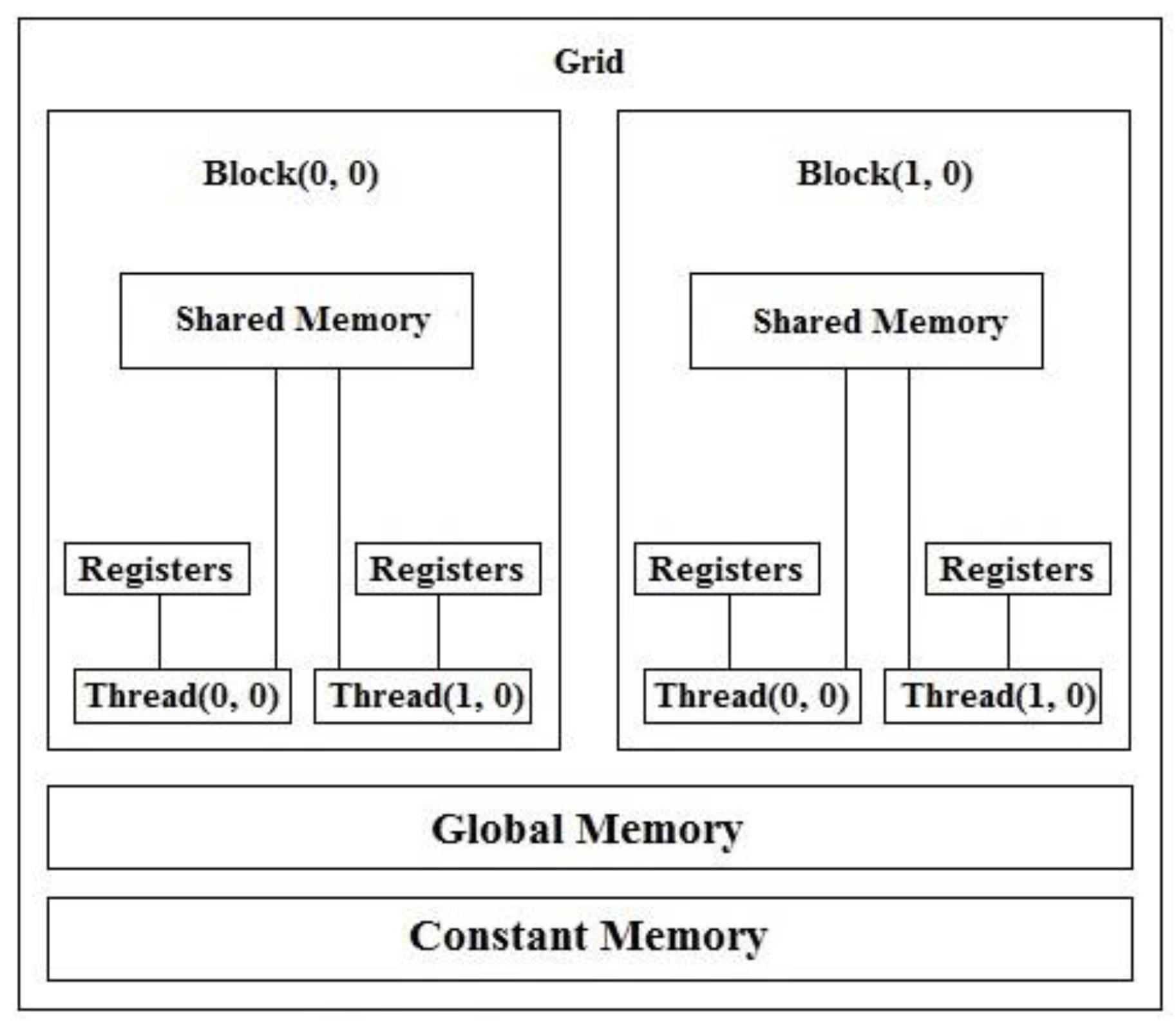
The GPU architecture is different from the CPU architecture in terms of memory. The GPU has multiple memory types (or levels). The global memory is the slowest memory and is a read/write memory. The global memory can be accessed by all the threads within the grid. The constant memory is a read-only memory and it’s faster than global memory. The constant memory can be accessed by all the threads within the grid, just like the global memory. The shared memory is defined for each block. The shared memory can be accessed by all the threads within the block. Automatic variables are stored in registers. Registers are faster than the shared memory. Registers can be accessed only by the current thread. The compiler sometimes places automatic variables in the local memory—for example, an array created within the kernel is likely to be stored in the local memory. The local memory space resides in the global memory, however other threads can’t access it. Local memory accesses have the same high latency and low bandwidth as global memory accesses, so local memory is rarely used. The local memory is only accessible from the current thread. Registers are faster than the shared memory. The shared memory is faster than the constant memory. The constant memory is faster than the global memory. Figure 1 illustrates the memory hierarchy of the GPU.
1.2. CUDA
Compute Unified Device Architecture (CUDA) [2,3] is often mistaken for a programming language, or it might be thought of as an Application Programming Interface (API). In fact, CUDA is more than that. CUDA is a general purpose parallel computing platform created by NVIDIA in 2006. It aids software developers by allowing the compute engine in NVIDIA GPUs to solve a variety of complex problems faster and more efficient than CPUs. CUDA allows the software developer to parallelize some portions of the program’s code in order to make the program run faster [4]. CUDA can be viewed as a layer that enables software developers to access the GPU for the sake of executing compute kernels. CUDA is designed to work with various programming languages; i.e., C, C++, C#, FORTRAN, Java, Python, etc. [4]. This makes it possible for software developers who are experts in diverse programming languages to use the CUDA platform comfortably.
CUDA has numerous advantages over traditional general-purpose computation on GPUs. Some of these advantages are:
- Faster downloads and readbacks to and from the GPU.
- Scattered reads.
- Unified memory (CUDA 6.0 and above).
- Full support for integer and bitwise operations.
- Unified virtual memory (CUDA 4.0 and above).
- Shared memory—CUDA exposes a fast shared memory region that can be shared among threads.
One way to use CUDA kernels is mentioned in the following steps:
- The CPU allocates storage on the GPU (using cudaMalloc()).
- The CPU copies input data from the CPU to the GPU (using cudaMemcpy()).
- The CPU launches on the GPU multiple copies of the kernel on parallel threads to process the GPU data. A kernel is a Function (Serial program) that will run on the GPU. The CPU which launch the kernel on parallel threads.
- The CPU copies results back from the GPU to the CPU (using cudaMemcpy()).
- Use or display the output.
The following code is a simple GPU kernel (written in CUDA) called AddArrays that is used for the purpose of adding two integer arrays. In this case, the CPU launches on the GPU multiple copies of the AddArrays kernel on parallel threads (one kernel per thread) in order to perform the addition operation.
__global__ void AddArrays(int *d_Arr1, int *d_Arr2, int *d_sum, unsigned int Length)
{
 unsigned int Index = (blockDim.x * blockIdx.x) + threadIdx.x;
 if (Index < Length)
 {
  d_sum[Index] = d_Arr1[Index] + d_Arr2[Index];
 }
}
Although CUDA allows us to run millions of threads or more, programs that run on the GPU aren’t million times faster than the CPU for multiple reasons:
- It takes time to copy data from the CPU to the GPU and vice versa.
- CUDA doesn’t allow all the threads to run simultaneously on the GPU since it depends on the architecture of the GPU.
- Kernel threads access global memory which is implemented in Dynamic Random Access Memory (DRAM) (slow and there is a lookup latency).
1.3. Sparse Matrix-Vector Multiplication (SpMV)
SpMV is a substantial computational kernel that has numerous applications in a wide variety of scientific areas and fields. SpMV is the main step of some iterative solvers, such as conjugate gradient (CG) and generalized minimum residual (GMRES), that can be used to solve sparse linear systems. SpMV has the form of Ax = y [5], where A is an m by n (m rows and n columns) sparse matrix, x is a dense vector of length n, y is a dense vector (the result of SpMV) of length m. A sparse matrix is a matrix that most of its elements are zeros. A dense vector is a vector that most of its elements are non-zeros. The sparsity of the matrix is the number of zero-valued elements divided by the total number of elements in the matrix (1 minus the density of the matrix, the sum of the sparsity and the density should equal 100%). SpMV itself is not a complex algorithm [6], but it might take a huge amount of time especially when we deal with big matrices. When matrices are sparse, the algorithm wastes a great deal of time trying to multiply zero elements by vector elements and the sparser the matrix is (increasing sparsity), the more time is wasted.
A linear system (system of linear equations) is a collection of two or more linear equations that include the same set of variables. SpMV can be effectively used to solve small-scale to large-scale linear systems [7,8] (systems of linear equations) and eigenvalue problems that have strong existence in a big variety of scientific applications, the matter that promotes the need to efficiently improve the SpMV operation on the GPU. As a matter of fact, improving the SpMV operation is extremely critical to the performance of a variety of scientific applications.
1.4. The Schrödinger Equation
The Schrödinger equation is a mathematical equation that can be used to study quantum mechanical systems, and it is well-known that any quantum mechanical system can be described and represented using this equation. The Schrödinger equation is considered the core of any quantum mechanical system and it was named after Erwin Schrödinger, a scientist who derived the equation in 1925.
The Time-independent Schrödinger equation is illustrated below:
where:
- h: Planck’s constant (6.62607004 × 10⁻³⁴ J.s).
- = h/2 π.
- m: Mass.
- ∇2: Second Derivative.
- V: Potential Energy.
- ψ: Wavefunction.
There are various techniques and methods that are used to solve the Schrödinger equation (figuring out the wavefunction and the energy) for a quantum system. The Hartree-Fock (HF) method [9], also known as the self-consistent field (SCF) method, is an approximation method that is used to determine the wavefunction and the energy of a quantum system. In the HF method, there is an assumption that the wavefunction can be approximated using a single Slater determinant (a representation of the wavefunction). The HF solution is considered a starting point for many methods that deal with many-electron systems.
Hartree-Fock method:
where:
F C = S C E
- F: Fock operator
- C: Matrix (a wavefunction)
- S: Overlap matrix.
- E: Energy
Ecorr = ɛo − Eo
- Ecorr: Electron Correlation Energy.
- εo: True (exact) ground state energy.
- Eo: HF energy.
Post-HF methods are considered a group of methods that were created in order to improve the HF method. Electron correlation is the interaction among electrons in the electronic structure of a quantum system. Electron correlation is an accurate way of including the repulsions among electrons. Electron correlation is considered by post-HF methods as opposed to the HF method, where repulsions are averaged.
2. Configuration Interaction (CI)
Quantum chemistry, of which CI is a part of, has made important contributions to understanding environmental fates of pollutants. Quantum mechanical calculations of quantum chemistry had contributed to the greening of many chemical practices [10]. This could be done via replacing experiments with computation as green alternative. So, what is Configuration Interaction? Configuration Interaction [11] is a linear method for solving the nonrelativistic Schrödinger equation for quantum chemical multi-electron systems. Relativistic wave equations are applicable to massive particles at high energies and high velocities comparable to the speed of light. Unlike other techniques and methods that can only deal with the ground state, the CI method can deal with the ground state as well as multiple excited states. The term “Configuration” basically refers to the linear combination of Slater determinants that are used for the wavefunction. The term “Interaction” refers to mixing different electronic states. CI uses a linear combination of configuration state functions (CSFs), which isn’t the case with the Hartree-Fock method. The CI approach is related to the size-extensivity problem, which has significantly reduced the use of the CI approach. The CI matrix is a sparse matrix, and the bigger the CI matrix, the more electron correlation can be captured. However, due to the large size of the CI sparse matrix that is involved in CI computations, a good amount of the time spent on the eigenvalue computations is associated with the multiplication of the CI sparse matrix by numerous vectors which is basically known as SpMV.
The trial wavefunction is written as a linear combination of determinants with the expansion coefficients determined by requiring that the energy should be a minimum. The MOs (Molecular Orbitals) used for building the excited Slater determinants are taken from a HF calculation. Determinants can be Singly, Doubly, Triply, etc., excited according to the HF configuration.
2.1. The CI Matrix Elements
The CI matrix elements Hij can be evaluated by the strategy employed for calculating the energy of a single determinant used for deriving the HF equations. This involves expanding the determinants in a sum of products of MOs, thereby making it possible to express the CI matrix elements in terms of MO integrals. There are some general features that make many of the CI matrix elements equal to zero.
The Hamiltonian operator does not contain spin, thus if two determinants have different total spin, the corresponding matrix element is zero. This situation occurs if an electron is excited from an α spin-MO to a β spin-MO.
When the HF wavefunction is a singlet, this excited determinant is a triplet. The corresponding CI matrix element can be written in terms of integrals over MOs, and the spin dependence can be separated out. If there is a different number of α and β spin-MOs, there will always be at least one integral 〈a|b〉 = 0. That matrix elements between different spin states are zero may be fairly obvious. If we are interested in a singlet wavefunction, only singlet determinants can enter the expansion with non-zero coefficients. However, if the Hamiltonian operator includes for example the spin–orbit operator, matrix elements between singlet and triplet determinants are not necessarily zero, and the resulting CI wavefunction will be a mixture of singlet and triplet determinants.
If the system contains symmetry, there are additional CI matrix elements that become zero. The symmetry of a determinant is given as the direct product of the symmetries of the MOs. The Hamiltonian operator always belongs to the totally symmetric representation. Therefore, if two determinants belong to different irreducible representations, the CI matrix element is zero. This is again fairly obvious if the interest is in a state of a specific symmetry, only those determinants that have the correct symmetry can contribute.
The excited Slater determinants are generated by removing electrons from occupied orbitals, and placing them in virtual orbitals. The number of excited Slater Determinants (SDs) is thus a combinatorial problem, and therefore increases factorially with the number of electrons and basis functions. Consider for example a system such as H2O with a 6-31G(d) basis. There are 10 electrons and 38 spin-MOs, of which 10 are occupied and 28 are empty.
The number of SDs = 38!/[10! (38 − 10)!].
The number of determinants (or CSFs) that can be generated grows wildly with the excitation level! Even if the C2v symmetry of H2O is employed, there is still a total of 7,536,400 singlet CSFs with A1 symmetry. Table 1 displays the number of singlet configuration state functions (CSFs) as a function of excitation level for H2O with a 6-31G(d) basis.
In order to develop a computationally tractable model, the number of excited determinants in the CI expansion must be reduced. Truncating the excitation level at one (CI with Singles (CIS)) does not give any improvement over the HF result as all matrix elements between the HF wavefunction and singly excited determinants are zero. CIS is equal to HF for the ground state energy, although higher roots from the secular equations may be used as approximations to excited states. Only doubly excited determinants have matrix elements with the HF wavefunction different from zero, thus the lowest CI level that gives an improvement over the HF result is to include only doubly excited states, yielding the CI with Doubles (CID) model. Compared with the number of doubly excited determinants, there are relatively few singly excited determinants, and including these gives the CI Singles and Doubles (CISD) method. Computationally, this is only a marginal increase in effort over CID. Although the singly excited determinants have zero matrix elements with the HF reference, they enter the wavefunction indirectly as they have non-zero matrix elements with the doubly excited determinants.
Small systems at the CISD level result in millions of CSFs. The variational problem is to extract one or possibly a few of the lowest eigenvalues and eigenvectors of a matrix the size of millions squared. This cannot be done by standard diagonalization methods where all the eigenvalues are found. There are iterative methods for extracting one, or a few, eigenvalues and eigenvectors of a large matrix.
Configuration State Functions (CSFs) are a linear combination of SDs. Molecular Orbitals (MO) are one dimensional objects that are used to create N-dimensional Slater Determinants. If we have a product of MOs and apply the anti-symmetrizer operation to it, you will create a single N-dimensional SD.
2.2. The CI Matrix
In this section, we will talk about the CI matrix. We will take linear combinations of SDs.
where:
- |Φo>: CI wavefunction.
- |Ψo>: Hartree-Fock wavefunction.
- C: Some coefficient that is applied to a Slater Determinant (Ψ).
- |>: All the possible single excitations. An electron is excited from orbital a to orbital r.
- |>: All the possible double excitations.
- …: All the way up to n excitations (excite n electrons).
If we take that to N-electron excitations, then we will have what’s called Full CI. In the case of Full CI, we have every single electron and every possible Slater determinant using all the orbitals available to us. Full CI is considered the exact solution to the nonrelativistic Schrödinger equation within the basis set. If we truncate that at a lower order, if we only do Single Excitations, then we will have what’s called CIS, if we have Double Excitations, then we will have CISD, and this will continue until we reach Full CI.
The SD is used as a basis function. The Hamiltonian is expressed in the basis of these SDs. Therefore, we will diagonalize the Hamiltonian matrix and get the lowest eigenvalue from that to be our ground state.
The Hamiltonian matrix (CI matrix, H) will act on a vector of all of our coefficients (c) and gives the energy out (E) and the coefficients back. So, what does the Hamiltonian matrix look like? It looks like the following:
And this will continue all the way to N Full Excitations <N|H|N>. <Ψo|H|S> is the wavefunction interacting with single excitations. <Ψo|H|D> is the wavefunction interacting with double excitations.
For single excitations, if we have N electrons and K basis functions, the number of single excitations we will have will be:
The previous value can be very large depending on the number of electrons you have (N), and the number of basis functions you have. The total number of SDs you will get is:
For double excitations, if we have N electrons and K basis functions, the number of double excitations we will have will be:
Full CI is very expensive [12]. The scaling for Full CI is on the order of O(N!), where N is the number of electrons. Full CI is exponential with the number of electrons and also with the basis set sizes. Generally, both the number of electrons and the number of basis functions affect computational costs, but the number of basis functions is usually the limiting factor. The number of basis functions that we use depends on and scales with the number of atoms and the types of atoms. A small calculation would have 14 basis functions per carbon atom. A big calculation on Chromium might have 93 basis functions per atom.
2.3. The Proposed Work
One of the main issues in CI computations is the immensely huge size of the CI sparse matrix [13]. The construction of the CI sparse matrix is very expensive. Some of the elements of the CI matrix are hard to calculate or recreate and some are not. Different parts of the CI sparse matrix can be calculated using different ways, therefore we have two approaches. One approach would be to pre-calculate the sparse matrix once at the beginning [13]. This option fits some parts of the CI sparse matrix that are hard to recreate. Adopting this approach will be limited by the GPU memory. The other approach would be to calculate the elements of the CI sparse matrix on the fly. This option fits some parts of the CI sparse matrix that are easy to recreate. It’s worth mentioning that CPUs are faster than the GPUs when calculating the elements on the fly since CPUs have more complex chips than GPUs [14]. GPUs do branch prediction in a slower fashion than CPUs. CPUs have better caching and more caches than GPUs, whereas GPUs have only global memory (slow), constant memory, local memory, shared memory, and registers. Modern CI calculations are often done on the fly, but this doesn’t mean that the entire problem can be done on the fly. Based on the pre-mentioned information, we are going to develop a hybrid approach in order to deal with the CI sparse matrix elements.
In this paper, we have implemented an efficient and powerful format for storing CI sparse matrices on the GPU. The proposed format compresses the sparse matrix in a way that saves a considerable amount of GPU memory. Besides, we have developed the SpMV kernel for the proposed format on the GPU. The proposed SpMV kernel is a single SpMV vector kernel that assigns a warp to each single row in the Reference region (ELLPACK format) and assigns another warp to each single row in the Expansion Space region (CSR format). We used the C language [15] and the CUDA platform [2,3] for implementation. The C language is considered a fast high performance computing programming language as well as easy to use. Numerous programming languages as well as operating systems are built using the C language. The C language supports system calls more conveniently than FORTRAN. The two factors that we are interested in assessing and evaluating are the amount of used memory and performance [16].
3. Common Formats
The format in which the matrix is stored in the GPU memory affects both the performance of the SpMV operation and the amount of memory used. In this section, we will be discussing some of the features of various sparse matrix storage formats that are used for storing sparse matrices on the GPU. We will also be discussing the SpMV kernel that is used along with each format. Besides, we will take a look at the pros and the cons of each single storage format in terms of performance and the amount of used memory.
3.1. The CSR (Compressed Sparse Row) or CRS (Compressed Row Storage) Format
- The Value vector: Contains all the non-zero entries.
- The Column vector: Contains column index of each non-zero entry.
- The RowPtr vector: Contains the index of the first non-zero entry of each row in the “Value” vector. We add the number of non-zero entries in the sparse matrix as the last element of the RowPtr vector.
In terms of memory, the CSR format is very powerful and efficient since no zero-padding [19] is needed. In terms of performance, the CSR format is efficient for SpMV operations implemented on CPUs with multiple cores. On the other hand, on the GPU, the CSR format isn’t as efficient as the ELLPACK format and shows worse throughput than the ELLPACK format when it comes to SpMV due to the lack of coalesced access to global memory on the GPU [17].
Example:
Consider the following 6 by 5 sparse matrix A, where:
The three vectors will be:
- Value = 1, 2, 3, 4, 5, 6, 7, 8
- Column = 0, 2, 4, 1, 4, 2, 3, 4
- RowPtr = 0, 1, 3, 5, 6, 7, 8
Algorithm 1 describes the SpMV kernel for the CSR format.
| Algorithm 1 The SpMV kernel for the CSR format. |
| SpMV_CSR(Value, Column, Vector, RowPtr, Result) for i ← 0 to ROWS - 1 do Start ← RowPtr[i] End ← RowPtr[i + 1] for j ← Start to End - 1 do Temp ← Temp + (Value[j] * Vector[Column[j]]) Result[i] ← Temp Temp ← 0.00 |
3.2. The ELLPACK (ELL) Format
In the ELLPACK (ELL) format [17], each single row will have the same number of elements. If a row contains fewer non-zero elements, then it will be padded with zeros in order to reach the length of the longest non-zero entry row. For example, consider a 10 by 10 diagonal matrix (or an identity matrix) with the last row full of non-zero entries. In this case, each single row in the matrix except the last row will be padded with 9 zeros in order to reach the length of the longest non-zero entry row. Thus, instead of storing 19 elements in memory, we store 100 elements in memory.
The ELLPACK (ELL) format compresses a sparse matrix into two matrices:
- The NonZerosEntries matrix: All the non-zero entries.
- The Column matrix: The column index of each non-zero entry.
In terms of memory, the ELLPACK format introduces a noticeable redundancy since zero-padding [19] is needed in order to reach the length of the longest non-zero entry row. Therefore, the ELLPACK format is less efficient than the CSR format from the memory standpoint.
In terms of performance, the ELLPACK format achieves better performance on the GPU than on the CPU due to the coalesced access to global memory on the GPU [17]. To ensure coalesced global memory access on the GPU, the number of rows has to be a multiple of the block size. This can be achieved by adding extra rows with zero entries [17].
Example:
Consider the following 6 by 5 sparse matrix A, where:
The two matrices will be:
Algorithm 2 describes the SpMV kernel for the ELLPACK format (thread per row) [20].
| Algorithm 2 The SpMV kernel for the ELLPACK format (thread per row). |
| SpMV_ELLPACK(NonZerosEntries, Column, Vector, Result, MaxNonZeros) for r1 ← 0 to ROWS – 1 do for r2 ← 0 to MaxNonZeros – 1 do if Column[r1][r2] = -1 then exit loop Temp = Temp + (NonZerosEntries[r1][r2] * Vector[Column[r1][r2]]) Result[r1] ← Temp Temp ← 0.00 |
3.3. The ELLPACK-R (ELL-R) Format
The performance of the SpMV operation can be further improved by adding an extra vector that includes the number of non-zero entries in each row (NonZerosCount vector). In this case, No iterations will be wasted in the loop since only non-zero entries will be involved in calculations [19].
Example:
Consider the following 6 by 5 sparse matrix A, where:
The three matrices will be:
Algorithm 3 describes the SpMV kernel for the ELLPACK-R format (thread per row).
| Algorithm 3 The SpMV kernel for the ELLPACK-R format (thread per row). |
| SpMV_ELLPACK_R(NonZerosEntries, Column, Vector, NonZerosCount, Result) for r1 ← 0 to ROWS – 1 do End ← NonZerosCount[r1] for r2 ← 0 to End – 1 do Temp ← Temp + (NonZerosEntries[r1][r2] * Vector[Column[r1][r2]]) Result[r1] ← Temp Temp ← 0.00 |
3.4. The Sliced ELLPACK Format
The Sliced ELLPACK Format was introduced in order to reduce the redundancy that is inherent in the ELLPACK Format. In this format, the matrix has to be divided first into submatrices (slices) and then each slice is stored in the ELLPACK format. Therefore, the number of extra zero entries (zero-padding) will be determined by the length of the longest non-zero entry row in each slice, rather than in the whole sparse matrix, so we will have less zero-padding, which definitely saves memory.
Example:
Consider the following 6 by 5 sparse matrix A, where:
Notice that we have one column in matrices, NonZerosEntries3 and Column3 instead of two, in other words, no zero-padding has occurred.
Algorithm 4 describes the SpMV kernel for the Sliced ELLPACK format (thread per row).
| Algorithm 4 The SpMV kernel for the Sliced ELLPACK format (thread per row). |
| SpMV_SlicedELLPACK(NonZerosEntries, Column, Vector, Result, Rows, Cols) for r1 ← 0 to Rows – 1 do for r2 ← 0 to Cols – 1 do if Column[r1][r2] = -1 then exit loop Temp ← Temp + (NonZerosEntries[r1][r2] * Vector[Column[r1][r2]]) Result[r1] ← Temp Temp ← 0.00 |
3.5. The Sliced ELLPACK-R Format
It’s worth mentioning that the Sliced ELLPACK format can be even further extended to be Sliced ELLPACK-R. In this case, the performance of the SpMV operation will be improved by adding an extra vector that counts the number of non-zeros in each row (NonZerosCount vector), just like the ELLPACK-R format.
Algorithm 5 describes the SpMV kernel for the Sliced ELLPACK-R format (thread per row).
| Algorithm 5 The SpMV kernel for the Sliced ELLPACK-R format (thread per row). |
| SpMV_SlicedELLPACK_R(NonZerosEntries, Column, Vector, NonZerosCount, Result, Rows) for r1 ← 0 to Rows – 1 do End ← NonZerosCount[r1] for r2 ← 0 to End – 1 do Temp ← Temp + (NonZerosEntries[r1][r2] * Vector[Column[r1][r2]]) Result[r1] ← Temp Temp ← 0.00 |
3.6. The Compressed Sparse Blocks (CSB) Format
The Compressed Sparse Blocks (CSB) format [13,21,22] is used for storing sparse matrices. The CSB format partitions the n × n matrix into n2/z2 equal-sized z × z square blocks using a block size parameter z. The CSB format consists of the following:
- The Value vector: The Value vector is of length nnz. It stored all the non-zero elements of the sparse matrix.
- The row_idx and col_idx vectors: They track the row index and the column index of each non-zero entry inside the Value vector with regard to the block, not the whole entire matrix. Therefore, row_idx and col_idx range from 0 to z – 1.
- The Block_ptr vector: It stores the index of the first non-zero entry of each block inside the Value vector.
4. The Proposed Model
The CI matrix is a sparse matrix that has a greatly-varying dimension length. It can be up to 107 by 107 or even more. Generally speaking, the CI matrix includes two main regions, namely, the Reference region and the Expansion Space region. The Reference region occupies almost 10% of the whole CI matrix with sparsity ranging from 70 to 80%. The Reference region starts out from the left side of the CI matrix. The Expansion Space region occupies the remaining space of the CI matrix with extremely high sparsity, which is around 98 to 99%.
4.1. The Proposed Storage Format
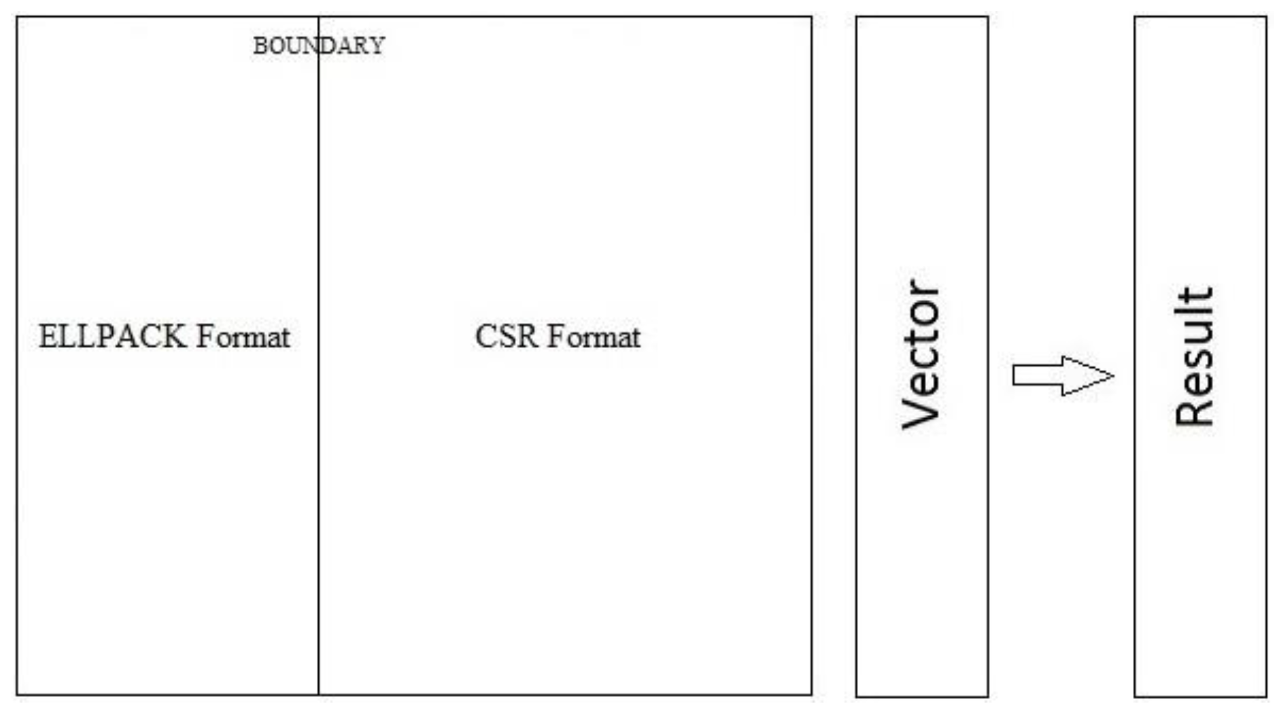
The proposed format is a combination of two formats: The ELLPACK format and the CSR format [8]. Each single row in the matrix is divided up into two sections based on the value of BOUNDARY. For each single row, columns with column indices ranging from 0 to (BOUNDARY–1) will be stored in the ELLPACK format and the rest of the row will be stored in the CSR format. The proposed format is illustrated in Figure 2.
The CSR format is very efficient with regard to using memory (storage space) since it does not require zero-padding like the ELLPACK format. Furthermore, the CSR format provides high performance for SpMV operations on CPUs that have multiple cores [17]. On the other hand, the CSR format provides lower performance than the ELLPACK format on GPUs when it comes to SpMV because of the lack of coalesced access to global memory on the GPU. The ELLPACK format provides higher performance than the CSR format on the GPU [17].
The Reference region of the CI matrix represents most of the electronic structure and performance is an important factor in this part, consequently we are going to store the Reference region in the ELLPACK format. The Expansion Space region that occupies the rest of the CI matrix has a noticeable high sparsity, so storage space is crucial and critical in this part. The CSR format is very powerful regarding storage space—therefore, the Expansion Space region will be stored in the CSR format. If we tried to store the Expansion Space region in the ELLPACK format, we will end up with a huge amount of zero-padding especially if one or more rows in the Expansion Space region was not/were not as sparse as the other rows in the same region.
As we saw in the previous figure (Figure 2), the value of BOUNDARY marks the end of the Reference region which is stored in the ELLPACK format and the beginning of the Expansion Space region which is stored in the CSR format.
Algorithm 6 describes the proposed format that we have created.
| Algorithm 6 The proposed format. |
| CreateFormat(Mat, NonZerosEntries, ELLPACK_Column, Value, CSR_Column, AllNonZerosCount, StartArr, EndArr) for i ← 0 to ROWS – 1 do c = 0 GotIt = 0 for j ← 0 to COLS – 1 do if Mat[i][j]! = 0.00 then if c < BOUNDARY NonZerosEntries[r][c] = Mat[i][j] ELLPACK_Column[r][c] = j c++ else Value[Index] = Mat[i][j] CSR_Column[Index] = j if GotIt = 0 GotIt = 1 Start = Index Index++ r++ if AllNonZerosCount[i] > BOUNDARY End = Index StartArr[i] = Start EndArr[i] = End |
The proposed model can calculate the amount of allocated memory that the proposed format uses. The space allocated to the proposed storage format can be calculated through the following equation:
where:
Storage Space = (3 × ROWS × sizeof(unsigned int)) + (ROWS × BOUNDARY ×
sizeof(double)) + ROWS × BOUNDARY × sizeof(int)) + (CSRNonZeros ×
sizeof(double)) + (CSRNonZeros × sizeof(unsigned int))
sizeof(double)) + ROWS × BOUNDARY × sizeof(int)) + (CSRNonZeros ×
sizeof(double)) + (CSRNonZeros × sizeof(unsigned int))
- ROWS: The number of rows in the matrix.
- BOUNDARY: A divider between the Reference region (ELLPACK format) and the Expansion Space region (CSR format). It marks the end of the Reference region and the start of the Expansion Space region.
- CSRNonZeros: The number of non-zero entries in the Expansion Space region.
The space allocated to the CSR storage format can be calculated through the following equation:
where:
Storage Space = (AllNonZeros × sizeof(double)) + (AllNonZeros × sizeof(unsigned
int)) + ((ROWS + 1) × sizeof(unsigned int))
int)) + ((ROWS + 1) × sizeof(unsigned int))
- AllNonZeros: The number of non-zero entries in the matrix.
- ROWS: The number of rows in the matrix.
The space allocated to the ELLPACK storage format can be calculated through the following equation:
where:
Storage Space = (ROWS × MaxNonZeros × sizeof(double)) + (ROWS ×
MaxNonZeros × sizeof(int))
MaxNonZeros × sizeof(int))
- ROWS: The number of rows in the matrix.
- MaxNonZeros: The length of the longest non-zero entry row in the matrix.
The Sliced ELLPACK Format was created in order to deal with the redundancy problem that exists in the ELLPACK Format. In this format, the matrix will be divided into submatrices (sometimes called slices) and then each submatrix will be stored in the ELLPACK format. The storage spaced that is allocated to the Sliced ELLPACK format will be the sum of the storage spaces that are allocated to the submatrices that make up the Sliced ELLPACK format. The sliced ELLPACK format takes less storage space than the ELLPACK format.
4.2. The Developed SpMV Kernel
The proposed storage format is used by our developed Warp-Based SpMV Kernel. The proposed SpMV kernel is a single SpMV vector kernel that assigns a warp to each single row in the Reference region, and assigns another warp to each single row in the Expansion Space region. Although scalar kernels (one thread per row) are relatively straightforward and provide reasonable performance, there is a big disadvantage that comes with them, when a thread accesses the elements of the storage format (by the storage format, we mean the vector that stores the values and the vector that stores the column indices), it accesses them in a sequential way. Every thread does not access these vectors simultaneously although they are stored in a contiguous fashion in the format, the matter that could have a negative effect on performance.
We overcame this problem when we developed the proposed SpMV kernel. The proposed SpMV kernel is a vector kernel that uses the warp approach, each row in each of the two regions of the storage format (Reference and Expansion Space regions) is accessed by a warp (32 threads), so in total, we have 2 warps that access each matrix row. The vector kernel eliminates the problem that is inherent in the scalar kernel (the threads’ sequential access to the values in the storage format). The order that Warps access the memory is difficult to determine and also does not affect performance. Furthermore, all warps execute independently in vector kernels, therefore thread divergence is less pronounced.
Each warp in the proposed SpMV kernel mandates coordination among the 32 threads that are within it, we achieved this using the atomicAdd() function. The atomicAdd() function provides a level of synchronization to the kernel, it reads a memory location and updates it and then stores the result back into the same location. Every thread has to wait on accessing that memory location until the atomicAdd() function is finished.
Algorithm 7 describes the SpMV kernel for the proposed format.
| Algorithm 7 The SpMV kernel for the proposed format. |
| SpMV_Hybrid_ELLPACKandCSR(NonZerosEntries, ELLPACK_Column, Value, CSR_Column, StartArr, EndArr, AllNonZerosCount, Vector, Result) Thread_id ← (blockDim.x × blockIdx.x) + threadIdx.x; Warp_id ← Thread_id/32 Th_Wa_Id ← Thread_id % 32 define ShMem1[32]//Shared Memory define ShMem2[32]//Shared Memory initialize ShMem1 initialize ShMem2 if Warp_id < ROWS then ShMem1[threadIdx.x] = 0.00 for r2 ← 0 + Th_Wa_Id to BOUNDARY – 1 STEP=32 do ShMem1[threadIdx.x] ← ShMem1[threadIdx.x] + (NonZerosEntries[Warp_id][r2] × Vector[ELLPACK_Column[Warp_id][r2]]) //Warp-level reduction for the ELLPACK format: if Th_Wa_Id < 16 ShMem1[threadIdx.x] ←(SynchronousAdd) ShMem1[threadIdx.x] + ShMem1[threadIdx.x + 16] if Th_Wa_Id < 8 ShMem1[threadIdx.x] ←(SynchronousAdd) ShMem1[threadIdx.x] + ShMem1[threadIdx.x + 8] if Th_Wa_Id < 4 ShMem1[threadIdx.x] ←(SynchronousAdd) ShMem1[threadIdx.x] + ShMem1[threadIdx.x + 4] if Th_Wa_Id < 2 ShMem1[threadIdx.x] ←(SynchronousAdd) ShMem1[threadIdx.x] + ShMem1[threadIdx.x + 2] if Th_Wa_Id < 1 ShMem1[threadIdx.x] ←(SynchronousAdd) ShMem1[threadIdx.x] + ShMem1[threadIdx.x + 1] if AllNonZerosCount[Warp_id] > BOUNDARY then Start ← StartArr[Warp_id] End ← EndArr[Warp_id] ShMem2[threadIdx.x] = 0.00 for j ← Start + Th_Wa_Id to End – 1 STEP=32 do ShMem2[threadIdx.x] ← ShMem2[threadIdx.x] + (Value[j] × Vector[CSR_Column[j]]) //Warp-level reduction for the CSR format: if Th_Wa_Id < 16 ShMem2[threadIdx.x] ←(SynchronousAdd) ShMem2[threadIdx.x] + ShMem2[threadIdx.x + 16] if Th_Wa_Id < 8 ShMem2[threadIdx.x] ←(SynchronousAdd) ShMem2[threadIdx.x] + ShMem2[threadIdx.x + 8] if Th_Wa_Id < 4 ShMem2[threadIdx.x] ←(SynchronousAdd) ShMem2[threadIdx.x] + ShMem2[threadIdx.x + 4] if Th_Wa_Id < 2 ShMem2[threadIdx.x] ←(SynchronousAdd) ShMem2[threadIdx.x] + ShMem2[threadIdx.x + 2] if Th_Wa_Id < 1 ShMem2[threadIdx.x] ←(SynchronousAdd) ShMem2[threadIdx.x] + ShMem2[threadIdx.x + 1] if Th_Wa_Id = 0 //Writing the results Result[Warp_id] ← Result[Warp_id] + ShMem1[threadIdx.x] + ShMem2[threadIdx.x] |
Thread_id is the index of each thread within the whole entire grid, Warp_id is the index of each warp within the grid, and Th_Wa_Id is the index of each thread inside the warp.
The overall memory is efficiently used throughout the use of shared memory. The shared memory (which is much faster than global memory) is useful if you access the data transferred to it more than once (which happens in the proposed model), using good access patterns, to have it help. If you access the data once, then the shared memory is not going to be useful. We computed the running sum for each thread in the Reference region by copying intermediate results to the shared memory (SharedMem1). We did the same thing with the Expansion Space region by copying intermediate results to the shared memory (SharedMem2). For the Reference region and the Expansion Space region, we had to perform parallel reduction in SharedMem1 and SharedMem2. The global memory is not accessed by every thread within the warp, instead we let the first thread in the warp (Th_Wa_Id = 0) access the global memory and write the results back to it by copying them from the shared memory (SharedMem1 and SharedMem2) to the global memory.
The proposed model generates some information about the CI matrix itself, i.e., the number of non-zero elements in the whole entire matrix, the number of non-zero elements in the Reference region (ELLPACK format), the number of non-zero elements in the Expansion Space region (CSR format), the number of non-zero elements in each row of the matrix, the number of non-zero elements in each row of the Reference region, the number of non-zero elements in each row of the Expansion Space region. It also outputs the length of the longest non-zero entry row in the whole entire matrix and its order as well. In addition to that, the proposed model calculates the amount of allocated memory that is used by the proposed format and the execution time that is consumed by the SpMV kernel. In addition to the results of the SpMV operation, the proposed model can produce the components of each of the storage formats (The ELLPACK format and the CSR format) that compose the hybrid format, if the user wanted to.
5. System Configuration
The proposed format and the developed kernel were both developed on Hodor supercomputer. Hodor has 33 compute nodes in total. 1 compute node is the head node. 16 out of the 33 compute nodes have NIVIDIA K20m GPUs. The remaining 16 compute nodes have Intel® Xeon Phi™ co-processor. The 16 compute nodes that have NIVIDIA K20m GPUs can be used to process CUDA code. Each compute node has the following configurations:
- NIVIDIA K20m GPU card or Intel® Xeon Phi™ co-processor card.
- 64 GB of memory.
- 150 GB RAID 17.2 K RPM storage hard drives.
- Linux Red Hat operating system RHEL 7.0.
Hodor supercomputer has an external 10 Gbps Ethernet communications network. In addition to that, it has an internal 56 Gbps Internal FDR InfiniBand network between the compute nodes. CUDA can be used in order to list the GPU properties. Table 2 lists the properties of the GPU in Hodor:
6. The Results
We have tested the proposed model with some simple and relatively large sparse matrices. We have compared the proposed format to the other common format using different-sized sparse matrices. Besides, we have compared the proposed kernel to the cuSPARSE library and the CSR5 (Compressed Sparse Row 5) format. The comparison was based on two main factors—the amount of used memory, and performance.
The output of the proposed model is very inclusive and comprehensive. It gives a lot of details about the format that is being used to store the sparse matrix on the GPU as well as the results of the SpMV operation. The information presented in the output is very intensive and elaborate.
We started out by using 10 CI sparse matrices for testing. Each sparse matrix is a 32,768 by 32,768 matrix (32,768 rows and 32,768 columns). Each single matrix was stored in different storage formats, namely the CSR format, the ELLPACK format, the Sliced ELLPACK format, and finally, the proposed format. We compared the proposed format to the other mentioned formats in terms of memory usage. We also compared the execution time of the proposed SpMV kernel to the execution times of the cuSPARSE library and the CSR5 format.
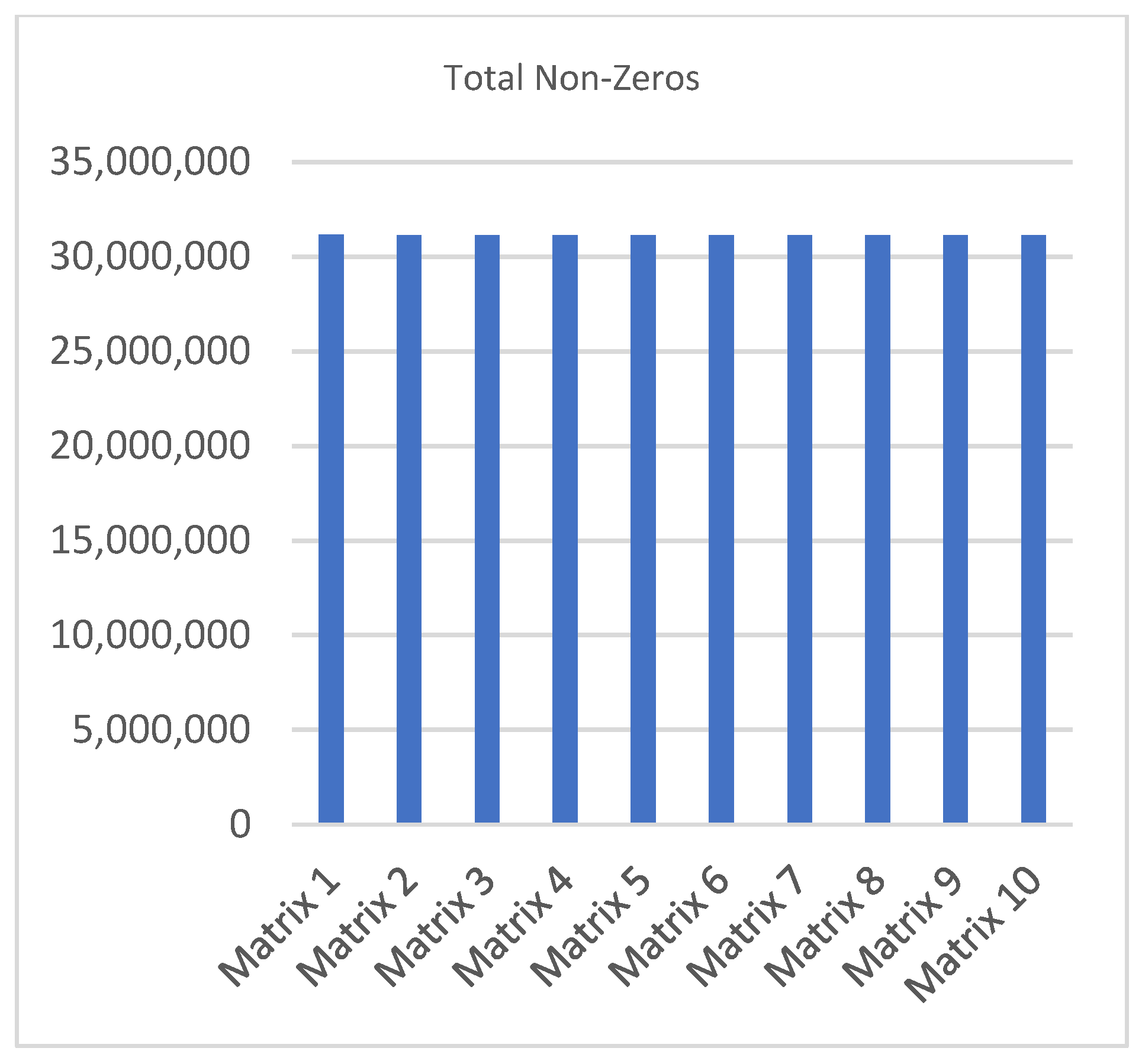
Table 3 demonstrates some general information about the 10 testing sparse matrices that will be stored in the proposed storage format. This information is about the number of non-zero entries in the Reference region, the number of non-zero entries in the Expansion Space region, and the total number of non-zero entries in the whole entire matrix.
The last column of Table 3 identifies the length of the longest non-zero entry row. In another way, the length of the row that has the largest number of non-zero elements in the whole entire sparse matrix. It also identifies the Row_Number of that row. Figure 3 shows the total number of non-zero entries in each of the 10 CI sparse matrices in a graphical way.
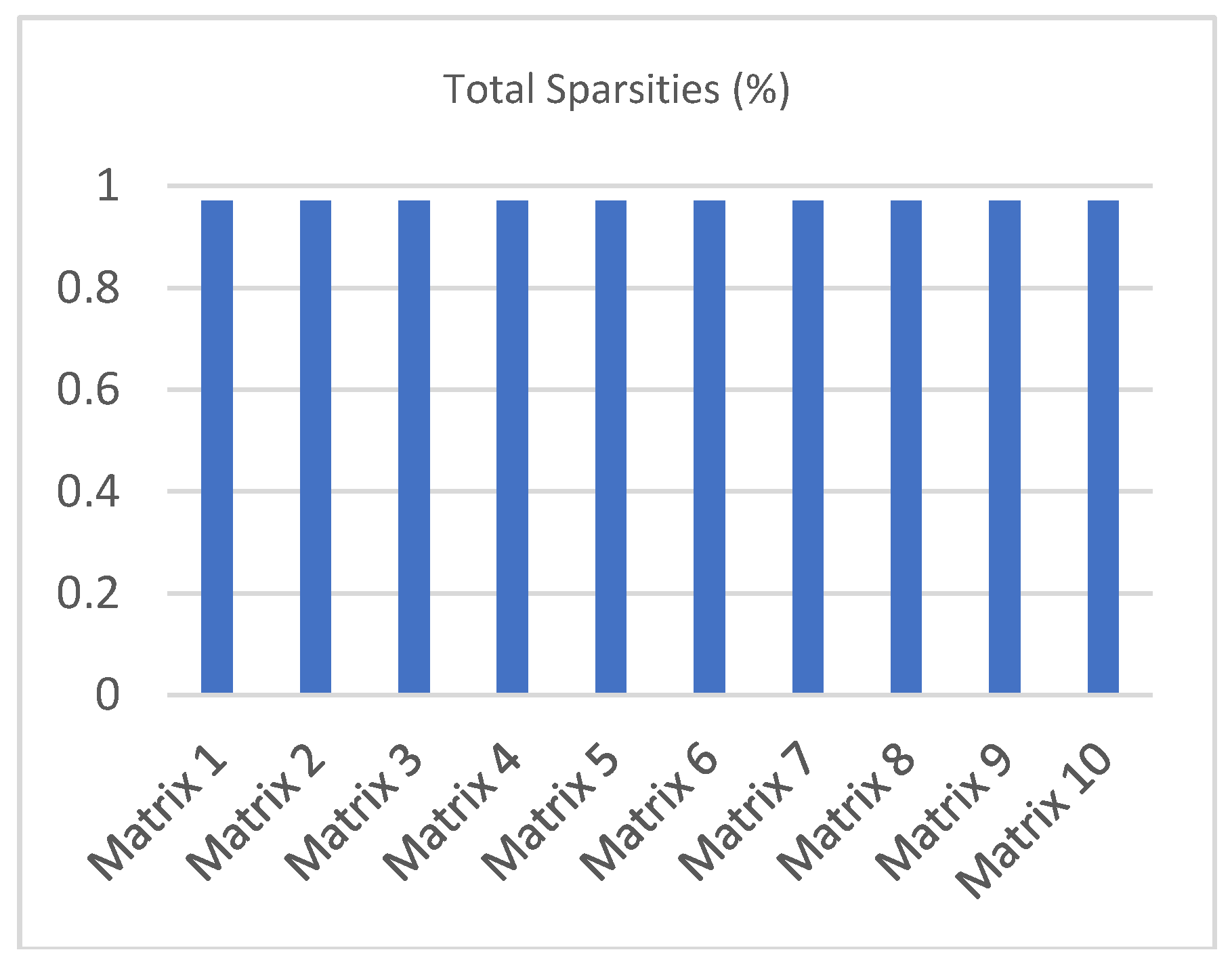
Table 4 shows some information about the sparsity of the 10 testing sparse matrices that will be stored in the proposed storage format. For each sparse matrix, it presents the sparsity of the Reference region, the sparsity of the Expansion Space region, and the overall total sparsity of the sparse matrix. Figure 4 shows the total sparsity of each of the 10 CI sparse matrices in a graphical way.
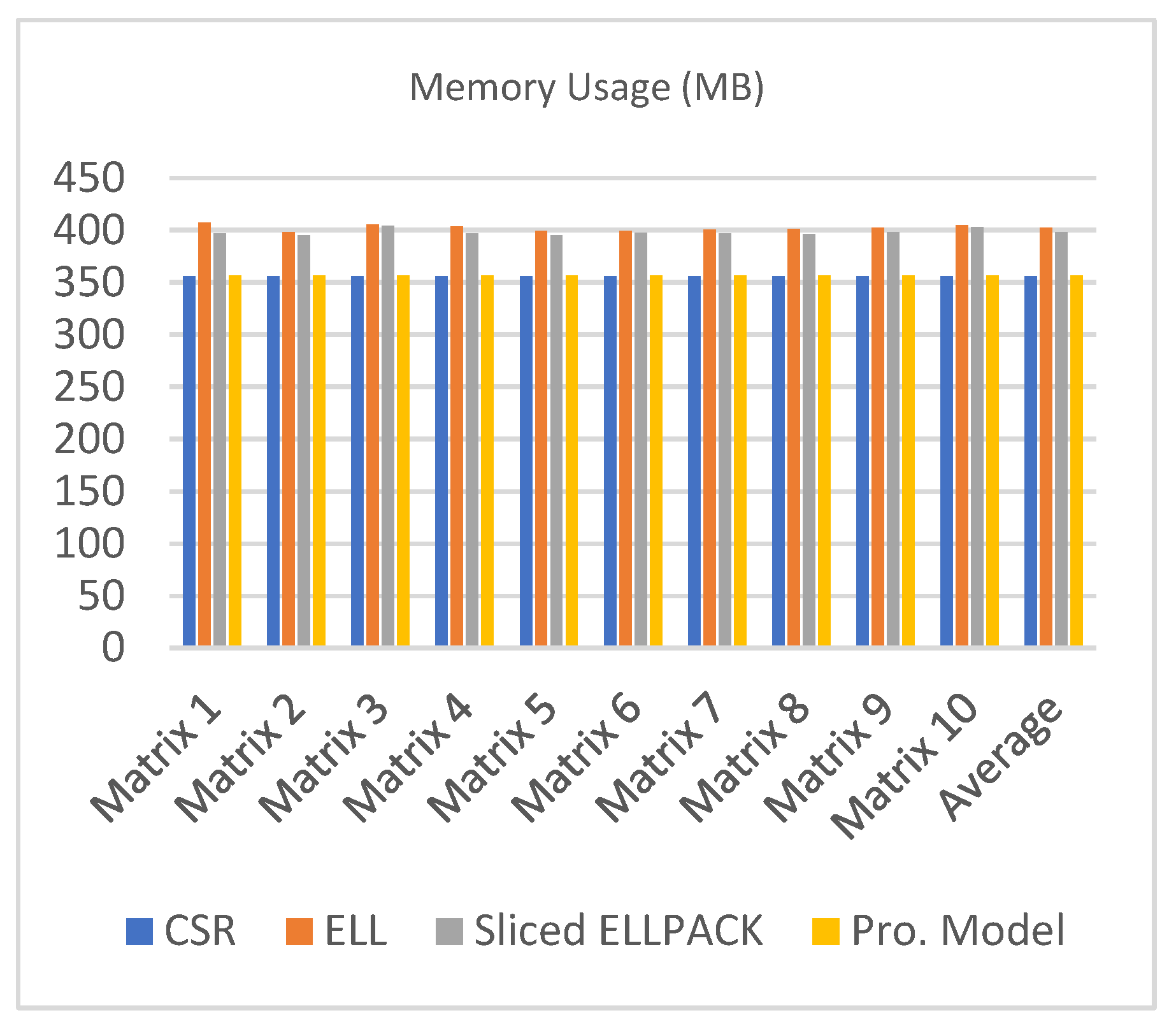
Table 5 compares the amount of memory used (in MB) by the proposed format to the amount of memory used by the CSR format, the ELLPACK format, and the Sliced ELLPACK formats. Figure 5 presents the same previous information (memory usage) in a graphical way.
In the following sections, performance will be the main point. We will discuss and analyze the performance of the proposed kernel and compare it to the other kernels.
The number of threads per block (block size) you choose can, and does effect the performance of the code that is running on the hardware. How each code behaves will be different and the only right way to quantify it, is by careful benchmarking and profiling. You should be aware that the block size you choose can and does have an impact on how fast your code will run, but it depends on the hardware you have and the code you are running. The number of threads per block should be a multiple of the warp size, which is 32 on all current hardware. In CUDA, in order to get the warp size for device number DevNo, you can use the following pseudocode:
- cudaDeviceProp DeviceProp_var
- cudaGetDeviceProperties(DeviceProp_var, DevNo)
- Print DeviceProp_var.warpSize
We are planning on using different values for the size of the block and then run our proposed CUDA SpMV kernel. Next, we will try to pick the block size that has the highest performance on the GPU. We tried 3 different block sizes for testing—16, 32, and 64. Finally, we will compare the proposed SpMV kernel with the best block size to the cuSPARSE library and the CSR5 (Compressed Sparse Row 5) format.
We used nvprof [23] which is a visual profiler developed by NIVIDIA, in order to analyze and view some performance data from the command line. We ran the proposed SpMV kernel with a block size (blockDim) of 16 and analyzed the performance using the nvprof tool. We used the nvprof tool while running the SpMV kernel using block sizes of 32 and 64 as well.
A subset of the output from the nvprof tool when we ran the proposed SpMV kernel using a block size of 16 is illustrated in Table 6. We had run the nvprof visual profiler 5 times.
Table 7 illustrates a subset of the output from the nvprof tool when we ran the proposed SpMV kernel using a block size of 32. We had run the nvprof visual profiler 5 times.
Table 8 illustrates a subset of the output from the nvprof tool when we ran the proposed SpMV kernel using a block size of 64. We had run the nvprof visual profiler 5 times.
In the previous experiments, we used the nvprof visual profiler while executing the proposed SpMV kernel and we considered different block sizes or different number of threads in each block. We tried three different block sizes of 16, 32, and 64. When the block size was set to 16, the average performance of the proposed SpMV kernel using the nvprof visual profiler was 4.8881 ms. When the block size was set to 32, the average performance of the proposed SpMV kernel using the nvprof visual profiler was 3.2844 ms. When the block size was set to 64, the average performance of the proposed SpMV kernel using the nvprof visual profiler was 3.5434 ms. The information presented in Table 6, Table 7 and Table 8, show that using the nvprof visual profiler while running the proposed SpMV kernel using a block size of 32 gives us the best performance, so we will consider this block size for testing.
In the next section, we tried to compare our proposed kernel to the cuSPARSE [24] library and the CSR5 (Compressed Sparse Row 5) format [25]. The cuSPARSE library was developed by NIVIDIA in order to perform linear algebra operations on matrices and vectors. It has already implemented subroutines that deal with the SpMV operation and it is easy to use. The cuSPARSE library supports multiple data types, i.e., float, double, cuComplex, and cuDoubleComplex. The cuSPARSE library supports multiple matrix data formats, i.e., the CSR format, the CSC format, the COO format, and the hybrid format which is a combination of 2 formats, the COO and the ELLPACK formats.
We used the cusparseDcsrmv() subroutine of the cuSPARSE library for the SpMV operation. The “D” portion in the subroutine name refers to the data type of the sparse matrix’s elements and the vector’s elements, which is double “double precision”, the “mv” portion refers to the fact that we multiply a matrix by a vector. If the elements of the sparse matrix and the vector are of type float “single precision”, then we can use the cusparseScsrmv() subroutine. The subroutines cusparseCcsrmv() and cusparseZcsrmv() deal with single precision and double precision complex numbers. The cuSPARSE library also supports matrix-matrix multiplication throughout the cusparseDcsrmm() subroutine that multiplies a sparse matrix (commonly a flat sparse matrix) by a dense matrix (commonly a tall dense matrix).
The CSR5 format [25] is insensitive to the sparsity structure of the sparse matrix. The SpMV kernel of the CSR5 format has high throughput on various platforms (CPU, the GPU, and Xeon Phi).
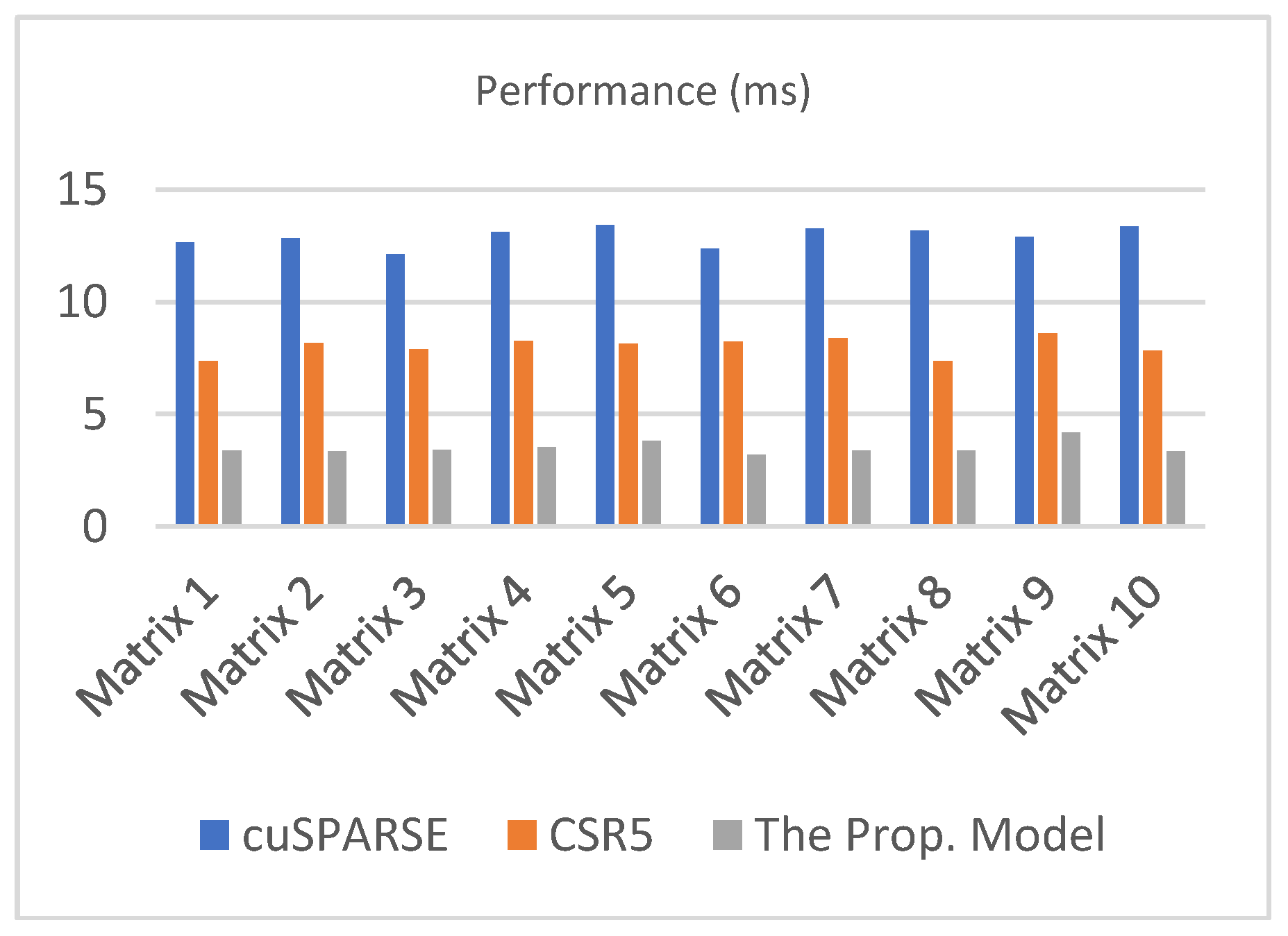
Table 9 compares the performance (in millisecond “ms”) of the proposed SpMV kernel to the performance of the cuSPARSE library and the CSR5 format. In this case, the block size (blockDim) is set to 32 for our proposed SpMV kernel, which means that each block will contain 32 threads. We ran the 3 SpMV kernels on the GPU and listed the results in the following table (Table 9). Figure 6 presents the same previous information (performance with a block size of 32) in a graphical way.
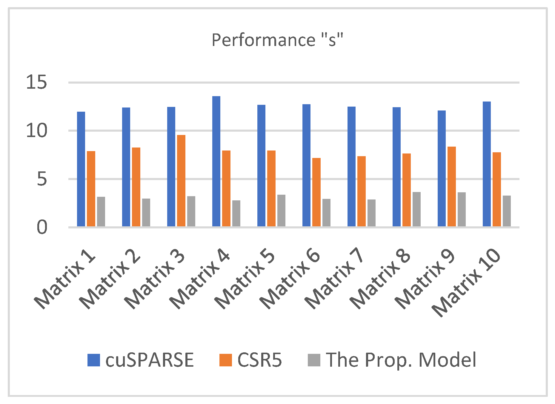
Since block size of 32 showed better performance, we tried to use it with bigger matrices. Subsequently, we tried to execute the proposed SpMV kernel using bigger matrices (1,048,576 by 1,048,576). We used the same block size which is 32. Table 10 compares the performance (in second “s”) of the proposed SpMV kernel to the cuSPARSE library and the CSR5 format using 10 different 1,048,576 by 1,048,576 CI sparse matrices. We ran the proposed SpMV kernel, the cuSPARSE library, and the CSR5 format on the GPU and listed the results in Table 10. Figure 7 presents the same previous information (performance in seconds with a block size of 32 using 10 different 1,048,576 by 1,048,576 CI sparse matrices) in a graphical way.
In general, with regard to memory usage, the proposed format used less memory than the ELLPACK format and the Sliced ELLPACK format and was too close to the CSR format. In terms of performance, the proposed kernel gained better performance than the cuSPARSE library and the CSR5 (Compressed Sparse Row 5) format when we used a block size of 32. The proposed SpMV kernel outperform the other kernels and we already showed that. If we tried to use the scalar ELLPACK kernel for our proposed model, the performance would have been very low since the number of non-zero entries in each row of the sparse matrix is not the same, the matter that leads to slowing the performance down significantly on the GPU. In the proposed model, the number of non-zero entries in each row of the ELLPACK format is guaranteed to be close, since each row starts out with the ELLPACK format’s (Reference region) elements followed by the CSR format’s elements, hence this guarantees high performance.
The CI sparse matrices are a special type of square sparse matrices that have a greatly-varying dimension length, they can be up to 107 by 107 or even more. CI sparse matrices have the same structure in terms of having two regions (the Reference Region and the Expansion Space Region) with two different sparsity settings. We used 20 matrices for testing, the first 10 matrices were 32,768 by 32,768, and the other 10 matrices were 1,048,576 by 1,048,576. For the first 10 matrices, they have different number of non-zero elements as illustrated in Table 3. The sparsity results in Table 4 look close because these matrices have a huge number of elements (1,073,741,824), and when dividing the number of non-zero elements by that number, in order to get the total sparsity of each CI sparse matrix The resulting percentages will look very close, which holds true for most CI matrices.
7. Conclusions
In this paper, we are proposing a new model for storing CI sparse matrices on the GPU. We have also implemented the kernel of the SpMV operation for the proposed model. We have started out by creating the storage format for the newly-developed proposed model. This storage format will be used to store CI matrices on the GPU. We have used this proposed format in order to develop the SpMV kernel for the proposed model. The previously-mentioned SpMV kernel will be used to multiply the compact representation of the CI sparse matrix by a vector. The proposed SpMV kernel that we have developed is a vector kernel that uses the warp technique. The proposed kernel was compared to the cuSPARSE library, and the CSR5 format using different input sparse matrices and already outperformed both of them. The proposed format used less memory than the ELLPACK format and the Sliced ELLPACK format.
The CI sparse matrices have a specific structure and the algorithm that we have developed is well-suited for them. The developed algorithm includes the use of two warps (one for each row in the Reference Region, and another warp for each row in the Expansion Space Region), with an efficient level of synchronization. The proposed algorithm didn’t use tiles as in CSR5, which is not a practical solution for CI matrices due to their irregular sparsity pattern through the whole entire matrix, rather used two warps that efficiently serve the two main regions of the CI matrix. Although the Expansion space region has a very small sparsity, it’s huge especially when we deal with big CI matrices, we stored the Expansion space region in the CSR format that is simple and uses very minimal space on the GPU compared to the CSR5 format.
8. Future Work
We are planning on updating the proposed model in order to deal with quaternion matrices (matrices whose elements are quaternions). Quaternions are 4-dimensional objects, where Q = [s, v], s ∈ R, v ∈ R3, Q = a + bi + cj + dk, a, b, c, d ∈ R. i2 = −1, j2 = −1, k2 = −1, ijk = −1. They extend complex numbers. When we move from complex numbers to quaternions, objects are no longer fields, whereas they algebraically form a semi-ring. We also lose commutativity. For example, ij = k whilst ji = −k. Subsequently, we will compare the proposed model (quaternions version) to other quaternions models. Of course, the comparison will be based on the two crucial key factors: The amount of used memory, and performance.
Author Contributions
M.M. is the first author on this paper. He was working with and advised by H.R. and M.H.
Funding
This research was funded by the Graduate School at the University of North Dakota.
Conflicts of Interest
The authors declare no conflict of interest.
References
- Mei, X.; Chu, X. Dissecting GPU Memory Hierarchy through Microbenchmarking. IEEE Trans. Parallel Distrib. Syst. 2017, 28, 72–86. [Google Scholar] [CrossRef]
- Nickolls, J.; Buck, I.; Garland, M.; Skadron, K. Scalable parallel programming with CUDA. In Proceedings of the ACM SIGGRAPH 2008 Classes, Los Angeles, CA, USA, 11–15 August 2008. [Google Scholar]
- NVIDIA Corporation. CUDA®: A General-Purpose Parallel Computing Platform and Programming Model. In NVIDIA CUDA Programming Guide; Version 2.0; NVIDIA: Santa Clara, CA, USA, 2008. [Google Scholar]
- NVidia Developer’s Guide, about CUDA. Available online: https://developer.nvidia.com/about-cuda (accessed on 2 October 2017).
- Kulkarni, M.A.V.; Barde, P.C.R. A Survey on Performance Modelling and Optimization Techniques for SpMV on GPUs. Int. J. Comput. Sci. Inf. Technol. 2014, 5, 7577–7582. [Google Scholar]
- Baskaran, M.M.; Bordawekar, R. Optimizing Sparse Matrix-Vector Multiplication on GPUs. Ninth SIAM Conf. Parallel Process. Sci. Comput. 2009; IBM Research Report no. RC24704. [Google Scholar]
- Bell, N.; Garland, M. Efficient Sparse Matrix-Vector Multiplication on CUDA. In Proceedings of the 2010 2nd International Conference on Education Technology and Computer, Shanghai, China, 22–24 June 2010. [Google Scholar]
- Guo, D.; Gropp, W.; Olson, L.N. A hybrid format for better performance of sparse matrix-vector multiplication on a GPU. Int. J. High Perform. Comput. Appl. 2016, 30, 103–120. [Google Scholar] [CrossRef]
- Echenique, P.; Alonso, J.L. A mathematical and computational review of Hartree-Fock SCF methods in quantum chemistry. Mol. Phys. 2007, 105, 3057–3098. [Google Scholar] [CrossRef] [Green Version]
- Anthony, B.M.; Stevens, J. Virtually going green: The role of quantum computational chemistry in reducing pollution and toxicity in chemistry. Phys. Sci. Rev. 2017, 2. [Google Scholar] [CrossRef]
- Siegbahn, P.E.M. The Configuration Interaction Method. Eur. Summer Sch. Quantum Chem. 2000, 1, 241–284. [Google Scholar]
- Alavi, A. Introduction to Full Configuration Interaction Quantum Monte Carlo with Applications to the Hubbard model Stuttgart. Autumn Sch. Correl. Electrons 2016, 6, 1–14. [Google Scholar]
- Aktulga, H.M.; Buluc, A.; Williams, S.; Yang, C. Optimizing sparse matrix-multiple vectors multiplication for nuclear configuration interaction calculations. In Proceedings of the 2014 IEEE 28th International Parallel and Distributed Processing Symposium, Phoenix, AZ, USA, 19–23 May 2014. [Google Scholar]
- Zardoshti, P.; Khunjush, F.; Sarbazi-Azad, H. Adaptive sparse matrix representation for efficient matrix-vector multiplication. J. Supercomput. 2016, 72, 3366–3386. [Google Scholar] [CrossRef]
- Ren, Z.; Ye, C.; Liu, G. Application and Research of C Language Programming Examination System Based on B/S. In Proceedings of the 2010 Third International Symposium on Information Processing, Qingdao, China, 15–17 October 2010. [Google Scholar]
- Bell, N.; Garland, M. Implementing sparse matrix-vector multiplication on throughput-oriented processors. In Proceedings of the Conference on High Performance Computing Networking, Storage and Analysis, Portland, OR, USA, 14–20 November 2009. [Google Scholar]
- Dziekonski, A.; Lamecki, A.; Mrozowski, M. A memory efficient and fast sparse matrix vector product on a GPU. Prog. Electromagn. Res. 2011, 116, 49–63. [Google Scholar] [CrossRef]
- Ye, F.; Calvin, C.; Petiton, S.G. A study of SpMV implementation using MPI and OpenMP on intel many-core architecture. In VECPAR 2014: High Performance Computing for Computational Science—VECPAR 2014; Lecture Notes in Computer Science Book Series; Springer: Cham, Switzerland, 2015; pp. 43–56. [Google Scholar]
- Maggioni, M.; Berger-Wolf, T. AdELL: An adaptive warp-Balancing ELL format for efficient sparse matrix-Vector multiplication on GPUs. In Proceedings of the 2013 42nd International Conference on Parallel Processing, Lyon, France, 1–4 October 2013. [Google Scholar]
- Eguly, I.R.; Giles, M. Efficient sparse matrix-vector multiplication on cache-based GPUs. In Proceedings of the 2012 Innovative Parallel Computing (InPar), San Jose, CA, USA, 13–14 May 2012. [Google Scholar]
- Buluç, A.; Fineman, J.T.; Frigo, M.; Gilbert, J.R.; Leiserson, C.E. Parallel sparse matrix-vector and matrix-transpose-vector multiplication using compressed sparse blocks. In Proceedings of the Twenty-First Annual Symposium on Parallelism in Algorithms and Architectures, Calgary, AB, Canada, 11–13 August 2009. [Google Scholar]
- Aktulga, H.M.; Afibuzzaman, M.; Williams, S.; Buluç, A.; Shao, M.; Yang, C.; Ng, E.G.; Maris, P.; Vary, J.P. A High Performance Block Eigensolver for Nuclear Configuration Interaction Calculations. IEEE Trans. Parallel Distrib. Syst. 2016, 28, 1550–1563. [Google Scholar] [CrossRef]
- CUDA Toolkit Documentation. nvprof. Available online: https://docs.nvidia.com/cuda/profiler-users-guide/index.html#nvprof-overview (accessed on 19 July 2018).
- CUDA Toolkit Documentation, cuSPARSE. Available online: https://docs.nvidia.com/cuda/cusparse/index.html (accessed on 16 July 2018).
- Liu, W.; Vinter, B. CSR5: An Efficient Storage Format for Cross-Platform Sparse Matrix-Vector Multiplication Categories and Subject Descriptors. In Proceedings of the 29th ACM on International Conference on Supercomputing, Newport Beach, CA, USA, 8–11 June 2015. [Google Scholar]
Figure 1.
The Graphics Processing Unit (GPU) memory hierarchy [1].
Figure 1.
The Graphics Processing Unit (GPU) memory hierarchy [1].

Figure 2.
The proposed format.

Figure 3.
Total zon-Zeros.

Figure 4.
Matrices total sparsity information.

Figure 5.
Memory usage.

Figure 6.
Performance with block size of 32.

Figure 7.
Performance with block size of 32 using 10 different 1,048,576 by 1,048,576 CI sparse matrices.
Figure 7.
Performance with block size of 32 using 10 different 1,048,576 by 1,048,576 CI sparse matrices.


Table 1.
The number of CSFs as a function of excitation level for H2O with a 6-31G(d) basis.
| Excitation Level (n). | Total Number of CSFs |
|---|---|
| 1 | 71 |
| 2 | 2556 |
| 3 | 42,596 |
| 4 | 391,126 |
| 5 | 2,114,666 |
| 6 | 7,147,876 |
| 7 | 15,836,556 |
| 8 | 24,490,201 |
| 9 | 29,044,751 |
| 10 | 30,046,752 |
Table 2.
GPU properties.
| Name | Tesla K20m |
|---|---|
| Major revision number | 3 |
| Minor revision number | 5 |
| Maximum memory pitch | 2,147,483,647 |
| Clock rate | 705,500 |
| Texture alignment | 512 |
| Concurrent copy and execution | Yes |
| Kernel execution timeout enabled | No |
| Number of multiprocessors | 13 |
| The maximum number of threads per multiprocessor | 2048 |
| The maximum number of threads per block | 1024 |
| The maximum sizes of each dimension of a block (x, y, z) | 1024, 1024, 64 |
| The maximum sizes of each dimension of a grid (x, y, z) | 2,147,483,647, 65,535, 65,535 |
| The total number of registers available per block | 65,536 |
| The total amount of shared memory per block (Bytes) | 49,152 |
| The total amount of constant memory (Bytes) | 65,536 |
| The total amount of global memory (Bytes), (Gigabytes) | 4,972,937,216, 4.631409 |
| Warp size (Threads) | 32 |
Table 3.
The proposed storage format information.
| Ref. Non-Zeros | Exp. Space Non-Zeros | Total Non-Zeros | Length of the Longest Non-Zero Row–Row No. | |
|---|---|---|---|---|
| Matrix 1 | 21,463,040 | 9,678,327 | 31,141,367 | 1074–5314 |
| Matrix 2 | 21,463,040 | 9,673,031 | 31,136,071 | 1069–6144 |
| Matrix 3 | 21,463,040 | 9,666,827 | 31,129,867 | 1078–22,358 |
| Matrix 4 | 21,463,040 | 9,670,529 | 31,133,569 | 1068–21,549 |
| Matrix 5 | 21,463,040 | 9,669,733 | 31,132,773 | 1060–4233 |
| Matrix 6 | 21,463,040 | 9,673,530 | 31,136,570 | 1069–28,394 |
| Matrix 7 | 21,463,040 | 9,666,857 | 31,129,897 | 1079–21,836 |
| Matrix 8 | 21,463,040 | 9,670,234 | 31,133,274 | 1077–20,148 |
| Matrix 9 | 21,463,040 | 9,661,419 | 31,124,459 | 1067–12,787 |
| Matrix 10 | 21,463,040 | 9,670,316 | 31,133,356 | 1064–25,678 |
Table 4.
Matrices sparsity information.
| Ref. Region Spar. (%) | Exp. Space Region Spar. (%) | Total Spar. (%) | |
|---|---|---|---|
| Matrix 1 | 0.800110 | 0.989985 | 0.970997 |
| Matrix 2 | 0.800110 | 0.989990 | 0.971002 |
| Matrix 3 | 0.800110 | 0.989997 | 0.971008 |
| Matrix 4 | 0.800110 | 0.989993 | 0.971005 |
| Matrix 5 | 0.800110 | 0.989994 | 0.971005 |
| Matrix 6 | 0.800110 | 0.989990 | 0.971002 |
| Matrix 7 | 0.800110 | 0.989997 | 0.971008 |
| Matrix 8 | 0.800110 | 0.989993 | 0.971005 |
| Matrix 9 | 0.800110 | 0.990002 | 0.971013 |
| Matrix 10 | 0.800110 | 0.989993 | 0.971005 |
Table 5.
Memory usage.
| CSR | ELL | Sliced ELLPACK | Pro. Model | |
|---|---|---|---|---|
| Matrix 1 | 356.44 | 407.25 | 397.13 | 356.76 |
| Matrix 2 | 356.46 | 398.25 | 395.06 | 356.70 |
| Matrix 3 | 356.39 | 405.75 | 404.44 | 356.63 |
| Matrix 4 | 356.49 | 403.88 | 397.03 | 356.67 |
| Matrix 5 | 356.39 | 399.38 | 395.06 | 356.66 |
| Matrix 6 | 356.38 | 399.75 | 397.59 | 356.70 |
| Matrix 7 | 356.45 | 400.88 | 396.94 | 356.63 |
| Matrix 8 | 356.51 | 401.25 | 396.56 | 356.67 |
| Matrix 9 | 356.43 | 402.75 | 398.25 | 356.57 |
| Matrix 10 | 356.44 | 405 | 403.13 | 356.67 |
| Average | 356.44 | 402.41 | 398.12 | 356.67 |
Table 6.
Running the nvprof profiler with a block size of 16.
| Block Size | Min | Max | Avg |
|---|---|---|---|
| 16 | 4.8877 ms | 4.8877 ms | 4.8877 ms |
| 16 | 4.8884 ms | 4.8884 ms | 4.8884 ms |
| 16 | 4.8891 ms | 4.8891 ms | 4.8891 ms |
| 16 | 4.8882 ms | 4.8882 ms | 4.8882 ms |
| 16 | 4.8870 ms | 4.8870 ms | 4.8870 ms |
| Average | 4.8881 ms | ||
Table 7.
Running the nvprof profiler with a block size of 32.
| Block Size | Min | Max | Avg |
|---|---|---|---|
| 32 | 3.2847 ms | 3.2847 ms | 3.2847 ms |
| 32 | 3.2838 ms | 3.2838 ms | 3.2838 ms |
| 32 | 3.2843 ms | 3.2843 ms | 3.2843 ms |
| 32 | 3.2834 ms | 3.2834 ms | 3.2834 ms |
| 32 | 3.2859 ms | 3.2859 ms | 3.2859 ms |
| Average | 3.2844 ms | ||
Table 8.
Running the nvprof profiler with a block size of 64.
| Block Size | Min | Max | Avg |
|---|---|---|---|
| 64 | 3.5451 ms | 3.5451 ms | 3.5451 ms |
| 64 | 3.5424 ms | 3.5424 ms | 3.5424 ms |
| 64 | 3.5437 ms | 3.5437 ms | 3.5437 ms |
| 64 | 3.5410 ms | 3.5410 ms | 3.5410 ms |
| 64 | 3.5448 ms | 3.5448 ms | 3.5448 ms |
| Average | 3.5434 ms | ||
Table 9.
Performance with a block size of 32.
| cuSPARSE | CSR5 | The Prop. Model | |
|---|---|---|---|
| Matrix 1 | 12.6567 | 7.3672 | 3.3661 |
| Matrix 2 | 12.8334 | 8.1694 | 3.3573 |
| Matrix 3 | 12.1227 | 7.8954 | 3.4127 |
| Matrix 4 | 13.1043 | 8.2654 | 3.5434 |
| Matrix 5 | 13.4352 | 8.1489 | 3.8167 |
| Matrix 6 | 12.3672 | 8.2336 | 3.1884 |
| Matrix 7 | 13.2559 | 8.3962 | 3.3655 |
| Matrix 8 | 13.1655 | 7.3672 | 3.3784 |
| Matrix 9 | 12.8985 | 8.5934 | 4.1836 |
| Matrix 10 | 13.3568 | 7.8349 | 3.3471 |
| Average | 12.9196 | 8.0272 | 3.3661 |
Table 10.
Performance with block size of 16 using 10 different 1,048,576 by 1,048,576 CI sparse matrices.
Table 10.
Performance with block size of 16 using 10 different 1,048,576 by 1,048,576 CI sparse matrices.
| cuSPARSE | CSR5 | The Prop. Model | |
|---|---|---|---|
| Matrix 1 | 11.9564 | 7.8736 | 3.1583 |
| Matrix 2 | 12.3787 | 8.2376 | 2.9672 |
| Matrix 3 | 12.4513 | 9.5462 | 3.1987 |
| Matrix 4 | 13.5645 | 7.9456 | 2.7761 |
| Matrix 5 | 12.6587 | 7.9348 | 3.3762 |
| Matrix 6 | 12.7457 | 7.1764 | 2.9376 |
| Matrix 7 | 12.4874 | 7.3672 | 2.8729 |
| Matrix 8 | 12.4138 | 7.6327 | 3.6534 |
| Matrix 9 | 12.0845 | 8.3432 | 3.6249 |
| Matrix 10 | 13.0198 | 7.7482 | 3.2653 |
| Average | 12.5761 | 7.9806 | 3.1831 |
© 2018 by the authors. Licensee MDPI, Basel, Switzerland. This article is an open access article distributed under the terms and conditions of the Creative Commons Attribution (CC BY) license (http://creativecommons.org/licenses/by/4.0/).
Share and Cite
MDPI and ACS Style
Mahmoud, M.; Hoffmann, M.; Reza, H. Developing a New Storage Format and a Warp-Based SpMV Kernel for Configuration Interaction Sparse Matrices on the GPU. Computation 2018, 6, 45. https://0-doi-org.brum.beds.ac.uk/10.3390/computation6030045
AMA Style
Mahmoud M, Hoffmann M, Reza H. Developing a New Storage Format and a Warp-Based SpMV Kernel for Configuration Interaction Sparse Matrices on the GPU. Computation. 2018; 6(3):45. https://0-doi-org.brum.beds.ac.uk/10.3390/computation6030045
Chicago/Turabian StyleMahmoud, Mohammed, Mark Hoffmann, and Hassan Reza. 2018. "Developing a New Storage Format and a Warp-Based SpMV Kernel for Configuration Interaction Sparse Matrices on the GPU" Computation 6, no. 3: 45. https://0-doi-org.brum.beds.ac.uk/10.3390/computation6030045
Note that from the first issue of 2016, this journal uses article numbers instead of page numbers. See further details here.