Numerical Simulation on Flow Dynamics and Pressure Variation in Porous Ceramic Filter

Department of Mechanical Systems Engineering, Nagoya University, Chikusa, Furo 1, Nagoya, Aichi-ken 4648603, Japan
*
Author to whom correspondence should be addressed.
Computation 2018, 6(4), 52; https://0-doi-org.brum.beds.ac.uk/10.3390/computation6040052
Submission received: 6 September 2018
/
Revised: 19 September 2018
/
Accepted: 20 September 2018
/
Published: 20 September 2018
(This article belongs to the Section Computational Engineering)
Abstract
:Using five samples with different porous materials of Al2TiO5, SiC, and cordierite, we numerically realized the fluid dynamics in a diesel filter (diesel particulate filter, DPF). These inner structures were obtained by X-ray CT scanning to reproduce the flow field in the real product. The porosity as well as pore size was selected systematically. Inside the DPF, the complex flow pattern appears. The maximum filtration velocity is over ten times larger than the velocity at the inlet. When the flow forcibly needs to go through the consecutive small pores along the filter’s porous walls, the resultant pressure drop becomes large. The flow path length ratio to the filter wall thickness is almost the same for all samples, and its value is only 1.2. Then, the filter backpressure closely depends on the flow pattern inside the filter, which is due to the local substrate structure. In the modified filter substrate, by enlarging the pore and reducing the resistance for the net flow, the pressure drop is largely suppressed.
1. Introduction
So far, a great amount of energy has been consumed in transport facilities, including trucks, buses, and passenger cars. Especially, it is well admitted that diesel cars have contributed to a variety of industries and services to support our society. In comparison with gasoline engines, the advantage of diesel engines is that their fuel consumption rate is relatively lower. The disadvantage is that emissions of nitrogen oxide (NOx) and small particulates (particulate matters, PM) in diesel exhaust cause a serious public health problem, such as heart and lung disease, together with environmental pollution [1,2,3]. Thus, more stringent emission limit values for NOx and PM are needed. Last year, in Europe, new exhaust emissions standards, Euro 6d-TEMP, were set.
As a countermeasure for the reduction of PM emissions, a well-known diesel filter (diesel particulate filter, DPF) is used. It is a very efficient device for particle filtration [4,5,6]. Resultantly, the combustion-generated nanoparticles, mainly from the internal combustion engine, are removed [7,8,9,10,11], but inevitably, the deposited particles could be a barrier or block for the flow during the filtration, and the unexpected pressure rise may worsen the fuel consumption rate as well as the available torque. Thus, the filter regeneration process for oxidizing and removing deposited soot is needed periodically or continuously [12,13,14,15,16]. Simultaneously, incombustible materials, including components of minerals such as calcium, manganese, and sulfur compounds, are inevitably formed [17]. Then, the lubricant-derived ash always accumulates inside the DPF. It should be noted that, different from carbon particulate oxidation, ash accumulation is an irreversible process, which inevitably limits the filter’s service life. Therefore, based on the knowledge of the flow field inside the filter, it is important to optimize the filter structure, including pore size and porosity, for the reduction of filter backpressure in advance.
Usually, those filter designs, including any manufacturing, have been referred to data by experiments. The information on the physical and chemical data related with phenomena inside the filter may not be enough, which could improve the filtration durability together with its filtration efficiency. Alternatively, it is indispensable to take advantage of the information on numerical simulations of the real filter systematically. Nevertheless, by the commercial software or in-house CFD code based on the Navier–Stokes equations, it is very challenging and computationally intensive to conduct the flow simulation, because we need to consider the complex geometry of the filter substrate and internal pores [18]. Thus, for the simulation in the porous filter with particle deposition, we have adopted a lattice Boltzmann method (LBM) [13,14,16,19,20,21,22,23].
It is well known that the numerical approach for boundary conditions in the LBM are easy, which would be suitable for the fluid simulation in porous media [24]. Previously, we have conducted the soot deposition and oxidation to simulate the particle trap and filter regeneration by LBM [13,14,16,19,20,21,22,23]. In this study, focusing on the filter substrate structure, we tested three materials, Al2TiO5, SiC, and cordierite, in the numerical simulation. To consider the fluid dynamics in the real product, we applied X-ray CT scanning for the filter inner structure [13,14,16,21,22]. We chose five samples (see Table 1) to set the porosities such as the pore size systematically. They have different porosity, pore size, cell density, and wall thickness. By comparing the filter properties of different materials, we discussed the flow field in detail, which could be deeply related with the filter backpressure.
2. Numerical Method
2.1. Lattice Boltzmann Method
In this section, we explain the numerical procedure in the lattice Boltzmann simulation. The formula of the LBM corresponds to a simplification of the Boltzmann equation [24]. The original approach proposed in our previous work was used [25], which is described briefly in this paper. Here, only the flow field was evaluated by way of the distribution function of the pressure. To realize the porous media flow in the uneven ceramic filter substrate, the 3D model [26] was used, which was composed of 15 discrete velocities in the lattice space, expressed by
where cα (α = 1 to 15) is the velocity of each advection along the lattice coordinate. The evolution equation for the convection of the flow is
Here, the time step is δt. The variable of τ is the relaxation time for controlling the rate to the equilibrium distribution due to collision. The equilibrium distribution function, pαeq, is
where wα = 1/9 (α = 1:6), wα = 1/72 (α = 7:14), and w15 = 2/9. The sound speed, cs, is c/ with p0 = ρ0RT0 = ρ0cs2. Here, p0 and ρ0 are the pressure and density at the room temperature. In the simulation, the temperature was constant. The pressure and the velocity vector of u = (ux, uy, uz) were evaluated in terms of the low Mach number approximation [13], together with the ideal gas equation.
The relaxation time of τ in Equation (2) is related with the kinetic viscosity using ν = (2τ − 1)/6 c2δt, showing that Navier–Stokes equations are derived by the Chapman–Enskog procedure [24]. In the numerical code, all variables were converted to be dimensionless. Based on the similarity of the Reynolds number (Re = UinW/ν), the real values such as flow velocity, were obtained, where Uin is the inflow velocity of the diesel exhaust and W is the inlet width of the 3D simulation area.
2.2. Inner Structure of Filter Substrate
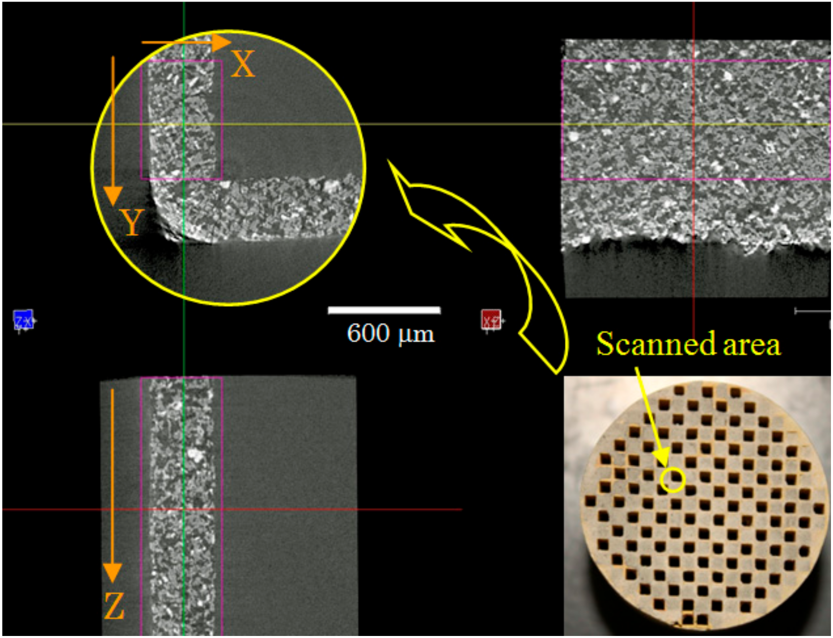
Our main advantage is that we would reproduce the exhaust gas flow in the real filter. Then, the data on the inner porous structure of the filter substrate was used in the simulation. Three materials of Al2TiO5, SiC, and cordierite with different porosity and pore size were tested. Table 1 shows filter properties of five samples. The porosity and the mean pore size were independently selected. In order to evaluate the flow field and the filter backpressure in the real filter, we applied the X-ray CT scanning. An example is shown in Figure 1, with the direct photograph of sample 1. As seen in the photograph, a part of the filter wall shown by the yellow circle was detected by the X-ray CT, and the three-dimensional substrate structure was obtained. In this figure, three slice images of sample 1 are shown. The coordinate system will be described later. The measurement resolution of the X-ray CT scanning was 1.42 μm/pix, which was the corresponding grid spacing in the numerical domain. Using CT data, it was possible to conduct the three-dimensional simulation to visualize the flow field inside the DPF. Since a part of the CT data was used in the simulation, convergence studies were conducted to set the proper numerical domain, which is explained later.
2.3. Numerical Domain
For the simulation, we used a standard PC with CPU of Intel Xeon Gold 5122 Processor (3.6 GHz), with multicore parallel computing. The numerical domain is shown in Figure 2, with the filter substrate of sample 1. At the inlet, the exhaust gas flowed along the X-direction normal to the filter wall. Besides, Y and Z were coordinates normal to X. As already explained, the grid size was 1.42 μm. In advance, for the convergence study, the total numerical domain was 500 μm (X) × W (Y) × W (Z), with inlet and outlet zones of 56 μm outside the filter wall. We changed the inlet width of W, and the inlet width in Figure 2 was W = 85 μm. To evaluate the filter backpressure, the simulation was continued to achieve the steady-state flow.
The boundary conditions are explained. At the filter inlet, the flow velocity (Uin) was given at 1 cm/s [13]. Different from previous simulations [13,14,16,19,20,21,22,23], only the flow was simulated, and the component of the exhaust gas was nitrogen. The temperature at the inlet (Tin) was 350 °C, which was used to determine the kinematic viscosity of the inflow. Each velocity component was set at ux = Uin, uy = 0, and uz = 0. On four side walls, we assumed the periodic structure of the porous material. Then, the slip boundary was adopted. At the exit (outlet), the pressure was always the atmospheric value. At the surface of the filter substrate, the nonslip wall boundary was used [27].
3. Results
3.1. Flow Field and Filter Backpressure
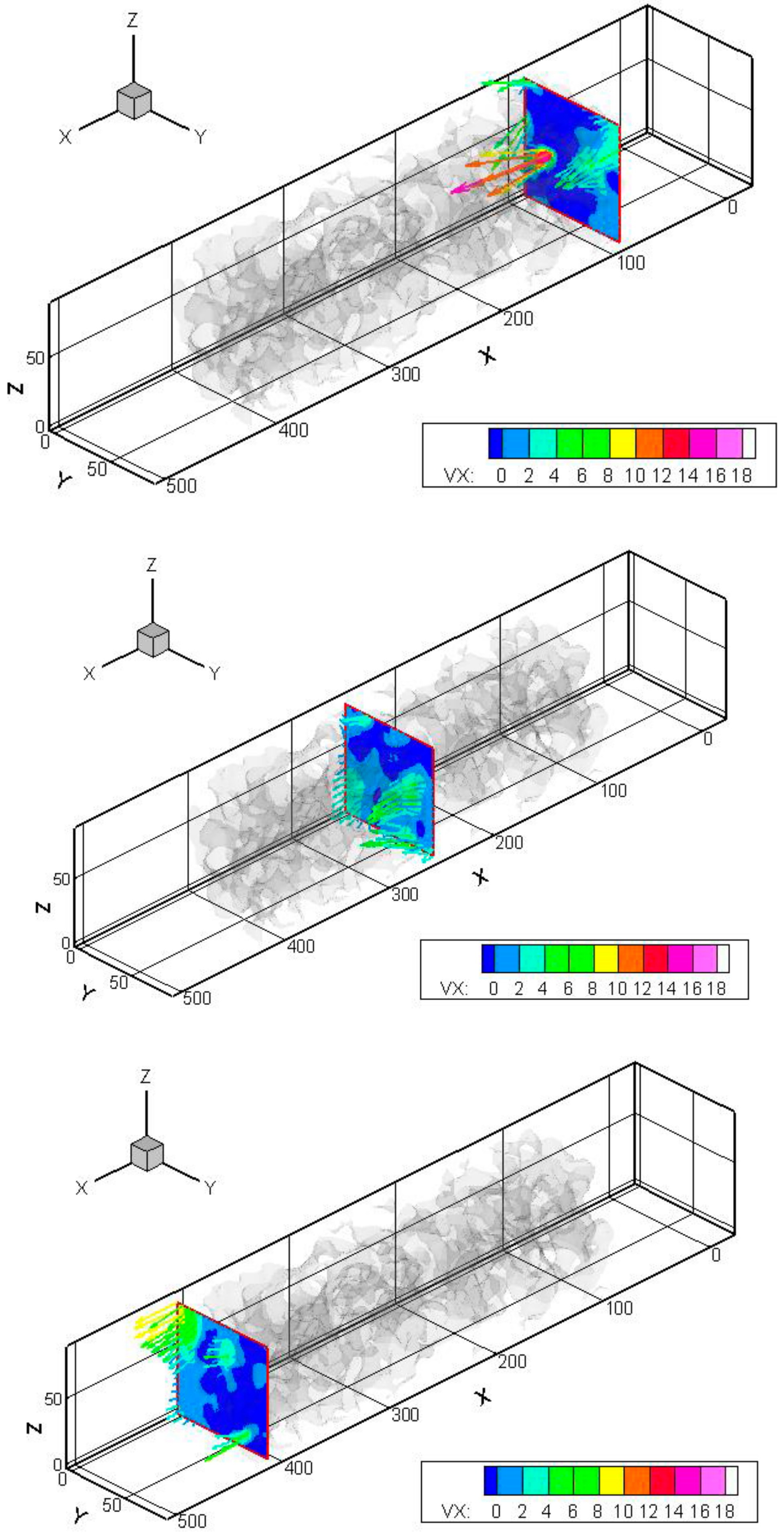
First, we visualized the flow field formed in the filter wall. Needless to say, the filter consisted of two or more interconnected porous substrates. Expectedly, the flow would be very complex inside the nonuniform structure of the filter wall. Figure 3 shows the flow velocity along X-direction at three different locations of sample 1. These were at X = 92, 255, 411 μm. The inlet width of W was 85 μm. It was seen that the flow was locally enlarged in the narrow area between pore spacing. Since the inlet velocity was 1 cm/s, the filtration velocity was much higher than the inflow velocity. Based on the flow trajectory inside the filter wall, it was found that there were a lot of stream paths along the filter substrate.
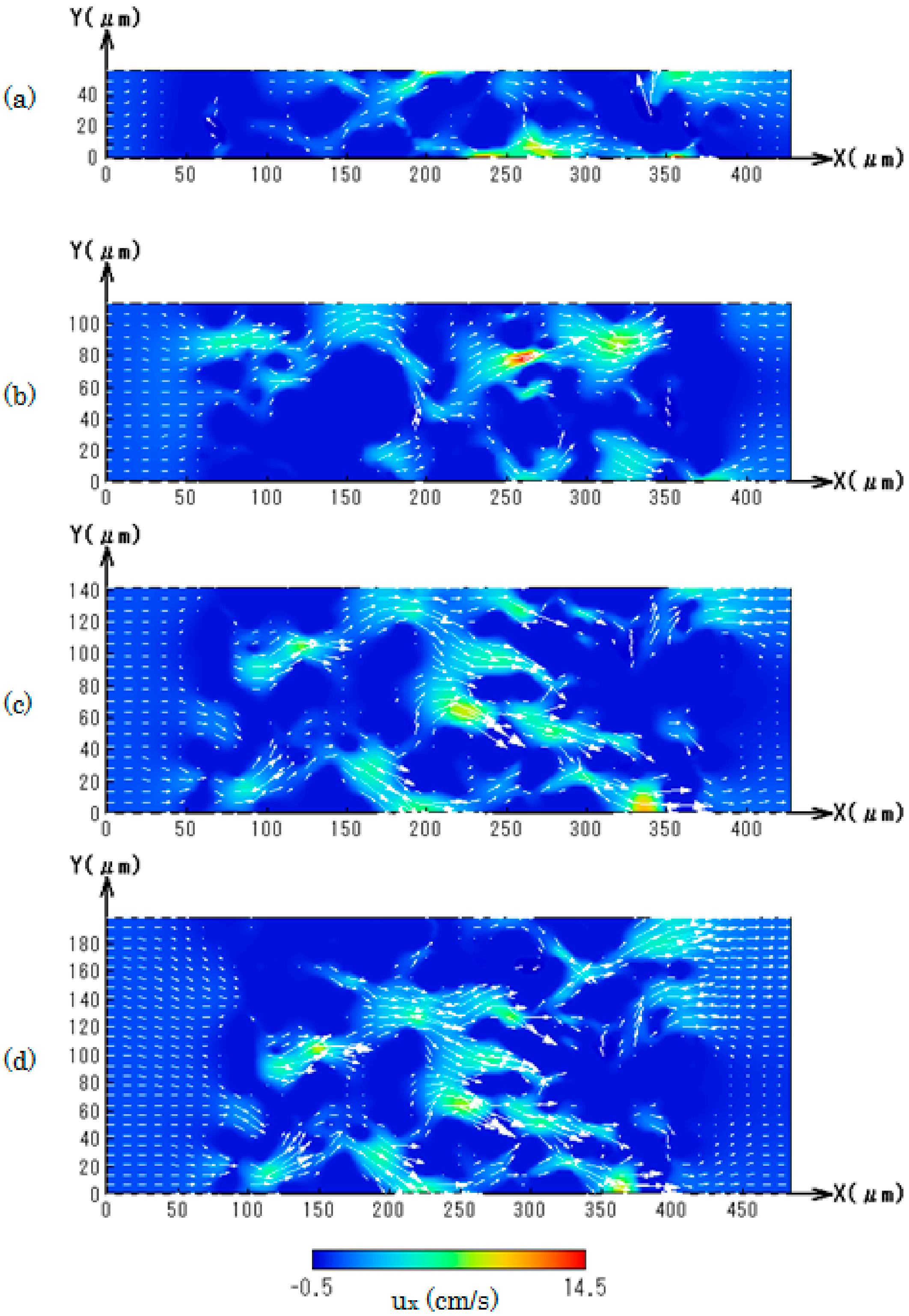
In the simulation, the computational time was roughly proportional to the total number of numerical grids. Then, only a small part of the filter wall obtained by the X-ray CT scanning was used, so that the long computational time would be avoided. Then, by considering that the numerical simulation was limited, a suitable numerical size should be selected. It is for the convergence study, and the dependence of the inlet width was investigated. Figure 4 shows distributions of ux with the velocity vector in XY plane at the center of the numerical domain with sample 1. The inlet width was changed at W = 57, 114, 142, 189 μm. The magnitude of the velocity is shown by the color from blue to red. The flow direction and its magnitude were largely changed, with the flow recirculation of negative velocity. Note that the inflow velocity was the smaller value of 1 cm/s, while the maximum flow velocity in the whole numerical domain was about 15 cm/s. Resultantly, the flow was largely accelerated, because the flow forcibly needed to go through the narrow pores in the filter wall, which is also seen in Figure 3. By comparing four figures, the clear difference was not observed. Then, by changing the inlet width of the filter, we checked the pressure distribution.
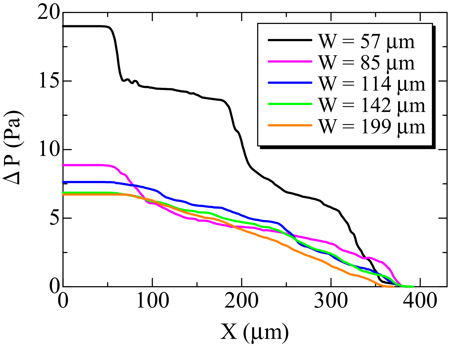
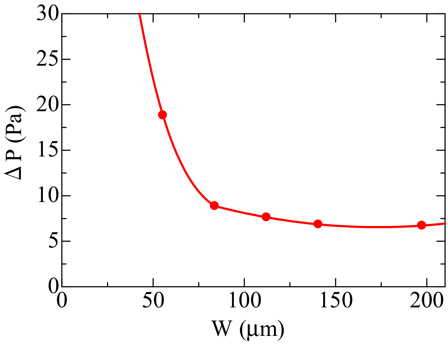
Results are shown in Figure 5. It is shown that when the inlet width was small, the pressure was largely varied. Especially, between four cases, the inlet pressure of the flow was quite different. As the inlet width was larger, the pressure at the inlet became lower. In other words, the filter backpressure was lower. Then, the filter backpressure was examined at the different inlet widths. Results are shown in Figure 6. It was found that, as W was increased, the filter backpressure became smaller, but it was saturated when W was greater than or equal to 85 μm. It should be noted that the same tendency was observed for the other four samples. It is considered that when the inlet area on the numerical domain was enlarged, more flow paths along the filter substrates appeared. However, the numerical domain was large enough, the similar velocity profile was observed, with the filter backpressure saturated. Hereafter, we set W to be 85 μm.
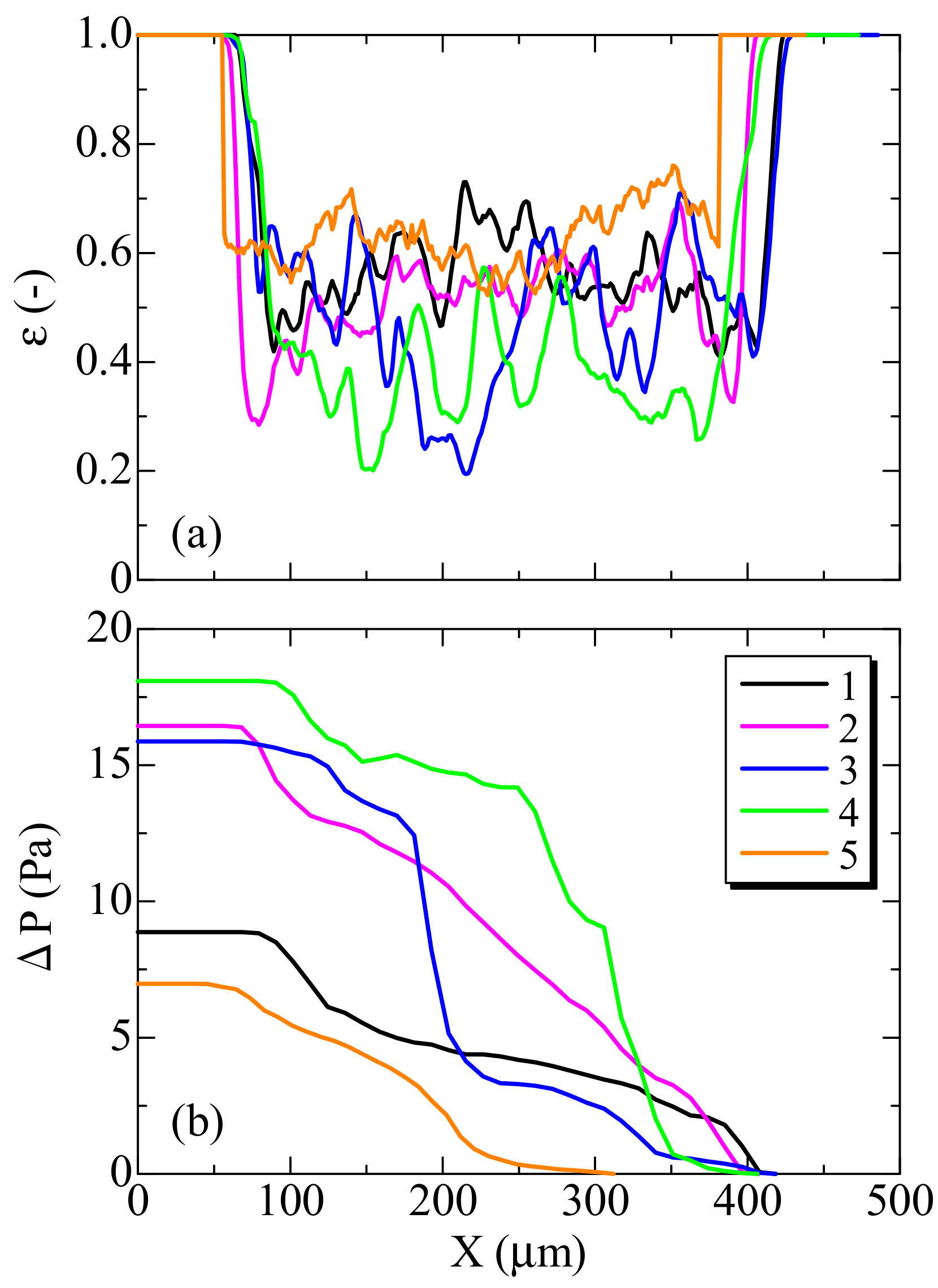
In Figure 7, the distributions of the porosity and the backpressure in the flow direction of X are shown. These describe the averaged variables in the YZ plane. The backpressure, Δp, is the pressure subtracted by the atmospheric pressure [16]. In Figure 7a, the porosity was locally varied, because the inner substrate structure was not uniform. Resultantly, in Figure 7b, the decreasing rate of the pressure was not constant. The filter backpressure was the lowest in sample 5 (cordierite), because the porosity was the highest and the filter wall thickness was thin. On the other hand, the filter backpressure of sample 4 (SiC) was the highest. At the same time, the porosity was the lowest and the average pore size was also small. By comparing the same material of samples 1 to 3, as the porosity as well as the pore size were smaller, the filter backpressure was found to be higher. Thus, the filter backpressure largely depends on the porosity and the pore size.
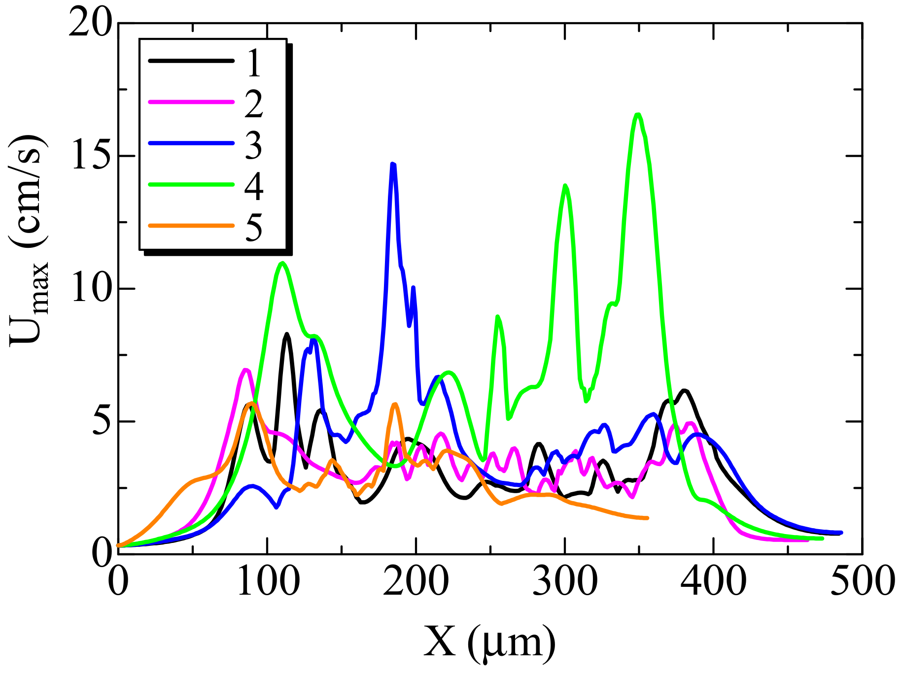
For further discussion on the filter backpressure, the filtration velocity observed in the filter wall was compared among five samples. Figure 8 shows the maximum filtration velocity measured in each YZ plane. The filtration velocity of U is expressed by
where ux, uy, uz are velocity components. Surprisingly, the maximum velocity was over 15 cm/s in sample 4, which exhibited the highest filter backpressure. Accordingly, the large acceleration of the filtration velocity was observed in the case of the filter with the high filter backpressure, because it was expected that there was the region of very narrow space between the filter substrates. The variation of the filtration velocity was also very large, compared with other samples. Conversely, in sample 5, whose filter backpressure was the lowest, the maximum filtration velocity was much smaller than that in the other four cases. Then, it could be derived that the filter backpressure is particularly related with the flow field. In the next section, the flow path is further examined.
U = (ux2 + uy2 + uz2)1/2
3.2. Flow Path Length inside DPF
In the complex structure of the filter substrate, there should be a lot of flow streams along the pores of the filter substrate. Then, we examined the flow path length quantitatively. Here, particles were added to visualize the flow pattern and the flow path length in the filter was counted. The formula of the particle motion is given by [28]
where ρp is the density of particles, dp is the particle diameter, V and u are the particle velocity and the flow velocity, respectively. In this formula, CD is the drag coefficient. By assuming the so-called Stokes’ Law, then CD = 24/Re, where Re is based on the particle diameter. Here, it was assumed that the density of particles was equal to the fluid density. The diameter of all particles was equivalent to 200 nm, which was small enough to follow the flow stream. The particle deposition by any interception effects was not included. In addition, since the flow was steady, it was easy to evaluate the flow path along the streamline by chasing the particle motion inside the filter wall. Before the simulation, initial positions of the particles were equally placed at all grids at the inlet.
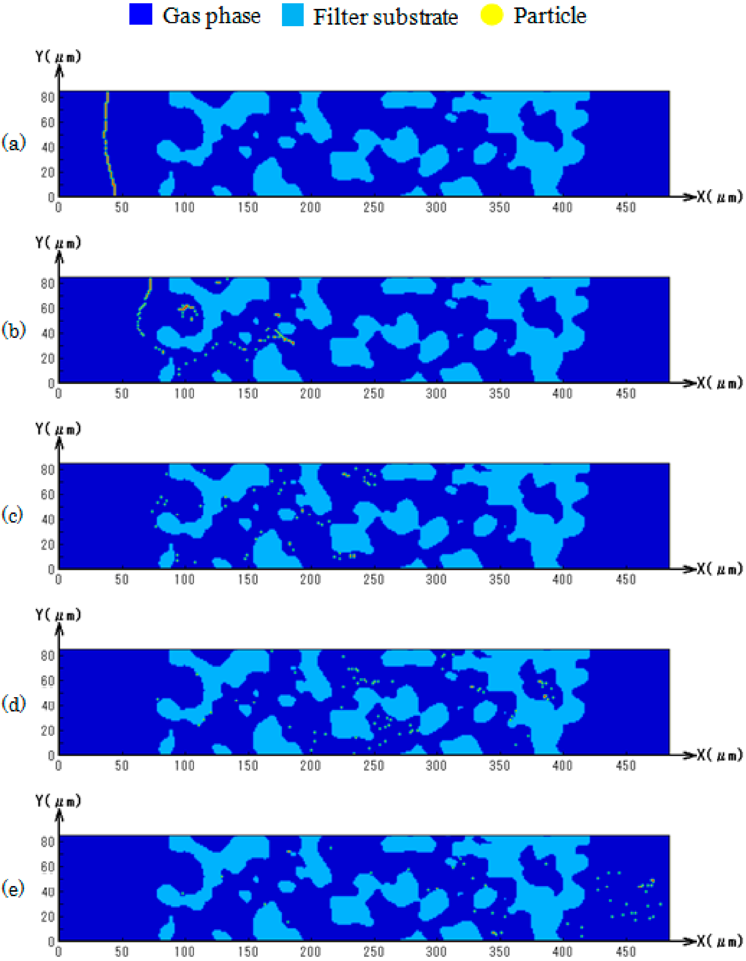
One example is described in Figure 9, showing the particle motion inside the filter. The particle positions at five different time steps are shown, where dots correspond to each particle location. These are the profiles at the central cross-section of the numerical domain at t = 4, 7, 11, 14, 21 ms. Since the filter has a three-dimensional structure, each particle could move freely into the substrate pore and never attach to the filter substrate. Even when we placed all particles at the inlet at t = 0 ms, the particle motion was transported by the convected flow, resulting in the very different motion inside the filter wall. Based on the trajectory of particles passing the filter wall, we discussed the flow path in each sample.
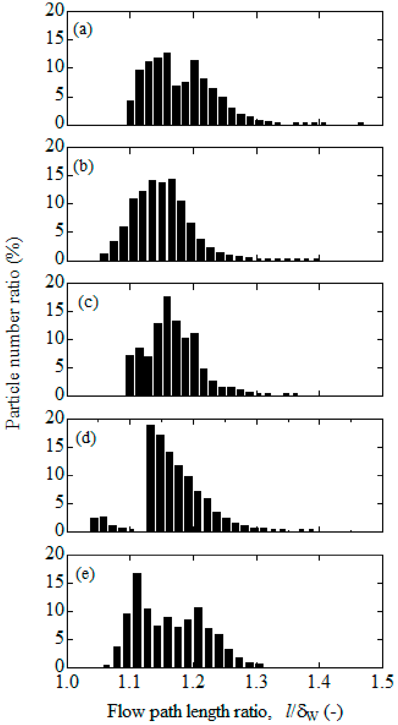
To discuss the flow field quantitatively, we estimated the flow path length, l. Here, the flow path length corresponds to the total length of the streamline calculated by the particle trajectory only inside the filter, which excludes the flow path at the region of inlet and outlet zones. Results are shown in Figure 10. Since each filter had a different filter wall thickness (δw), the flow path length was evaluated by the ratio to the filter wall thickness. We calculated the flow path length by using approximately 3600 particles. The ordinate was the value of particle numbers divided by the total particles in each range of the flow path length. Expectedly, the flow path could be longer when the particle moved along the complicated substrate structure. However, independent of the sample, the range of the flow path length was almost the same. Actually, the averaged value was 1.24, 1.20, 1.23, 1.24, and 1.23 for samples 1 to 5, respectively. That is, the flow path length was slightly longer than the wall thickness of the filter. Therefore, independent of the inner structure of the filter sample, the flow path length is almost constant.
4. Discussion
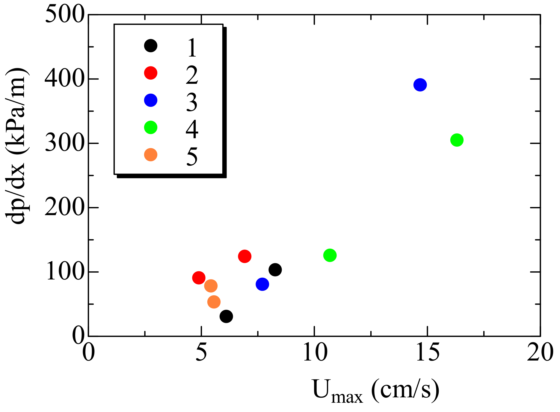
To design the filter with lower filter backpressure, the above information on the flow field must be useful. As shown in Figure 3 and Figure 4, at the region where the local space between substrates was much smaller, the local velocity was very high. That is, the flow velocity was steeply enlarged due to the narrower area along the porous wall. Then, it was difficult to go through the consecutive small pores along the filter’s porous walls, resulting in the large pressure drop. To confirm the above discussion, we examined the local pressure drop at the location where the velocity was significantly enlarged. Results are shown in Figure 11. It shows that there is a good relationship between the local pressure gradient and the maximum filtration velocity described by Equation (6). Two locations for each sample where the filtration velocity was locally the maximum were selected. To distinguish the results of each sample, color plots are used in this figure. Generally, the pressure gradient was larger when the local velocity was higher, although all plots are not on the same line. By considering each sample had different permeability, a good correlation in Figure 11 is quite an interesting finding.
Apparently, the pressure drop corresponding to the filter backpressure could be reduced as the overall porosity or the average pore size was larger. However, as shown in Figure 10, the flow path length across the filter wall of the different porous materials was almost the same. From the results in Figure 11, the further important point is that if the local porosity is not varied much, the smooth and uniform flow is achieved, ensuring that the large velocity fluctuation can be avoided. Thus, the filter backpressure closely depends on the flow pattern inside the filter, which is due to the local substrate structure. Especially, when the local pore size is very small, the pressure drop is inevitably enlarged. This specific location can be detected by examining the region where the local velocity is the maximum in Figure 8.
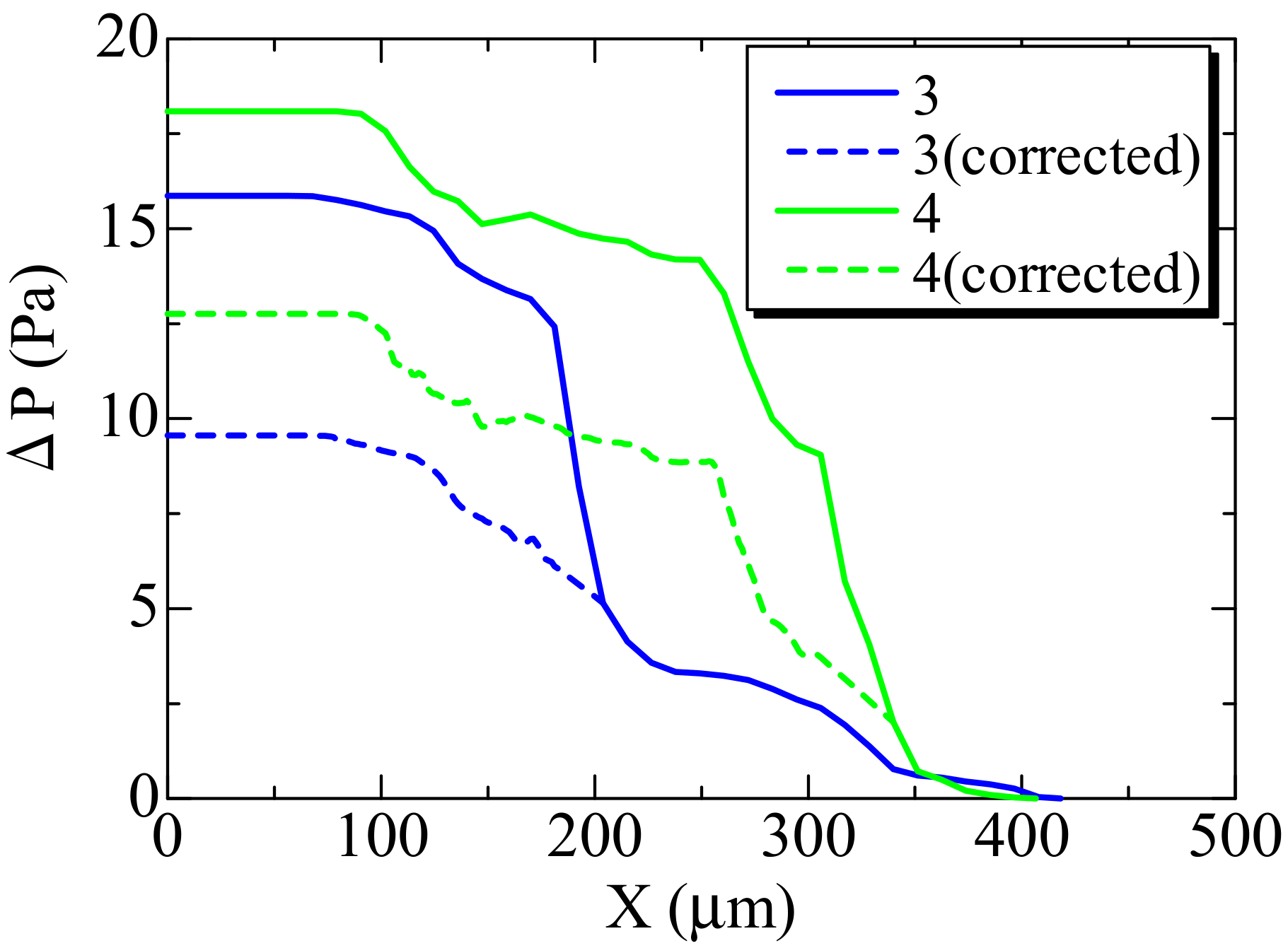
To confirm the above discussion, the filter substrate structure was modified. We selected two filters of samples 3 and 4, in which the large filter backpressure was observed. First, we specified the position with the large filtration velocity. In the case of sample 3, the small pore at which the flow was concentrated was located at around X = 200 μm. Besides, in the case of sample 4, that pore was located at X = 350 μm. These two pores could be crucial to show the bottleneck in the flow. That is, these pores showed some resistance for the net flow. Then, tentatively, two pores were enlarged to the mean pore size of 17 μm or 11 μm. The pressure distribution in the modified filter substrate is shown in Figure 12. For comparison, the original pressure distributions in Figure 7 are also shown. Apparently, the large pressure drop was avoided, resulting in the smaller filter backpressure. Therefore, if the bottleneck in the flow is more avoided, the pressure drop is significantly suppressed. Overall, the uniform pore structure is suitable to achieve the smooth velocity profile, resulting in the reduction of filter backpressure.
5. Conclusions
In this study, using five samples with different porous materials of Al2TiO5, SiC, and cordierite, we simulated the flow inside DPF. These inner structures were obtained by the X-ray CT scanning, in order to reproduce the real flow field in the porous filter. The following conclusions were drawn.
- (1)
- Inside DPFs, a complex flow pattern appears, with the large flow acceleration and the flow recirculation. In some areas, the maximum filtration velocity is over ten times larger than the inlet velocity of 1 cm/s. It is because the flow forcibly needs to go through the narrow pores along the porous filter wall, resulting in the large filter backpressure. By comparing 5 samples, it can be seen that the resultant pressure drop through the filter wall is smaller when the porosity or the pore size of the filter is larger.
- (2)
- To further discuss the flow field, the path length inside the DPF was estimated quantitatively. We followed the flow trajectory by tracing the particle motion in the fluid. The flow path length ratio to the filter wall thickness was almost the same for all samples, and its value was only 1.2. Therefore, independent of the porous material, the flow path length is almost constant under the present flow conditions.
- (3)
- The filter backpressure closely depends on the flow pattern inside the filter, which is due to the local substrate structure. In the modified filter substrate, by enlarging the pore size and reducing the resistance for the net flow, the pressure drop is largely suppressed. Therefore, when the local porosity is not varied much, the smooth and constant flow could be achieved, ensuring that the large velocity fluctuation is avoided. For the reduction of the filter backpressure, the uniform pore structure is suitable.
For the future design of DPFs, the above information could be useful to reduce the filter backpressure for particle filtration.
Author Contributions
K.Y. wrote the original draft, followed by the original idea for this numerical study. Y.T. was responsible for constructing the numerical code of the present simulation.
Funding
This research received no external funding.
Conflicts of Interest
The authors declare no conflict of interest.
Abbreviation
| Notation | |
| c | advection speed in lattice Boltzmann spacing |
| pα | distribution function of pressure |
| p | pressure |
| t | time |
| u | flow velocity of three components, u, v, w |
| Uin | inlet velocity |
| X | flow direction along the inflow |
| Y | direction perpendicular to X |
| Z | direction perpendicular to X |
| ε | porosity |
| ν | kinematic viscosity |
| ρ | density |
| τ | relaxation time |
| Subscripts | |
| 0 | reference condition at the atmosphere |
| in | value at inlet of numerical domain |
| p | value of particle |
| α | number of advection speed in LB coordinate |
References
- Wang, S.; Haynes, B.S. Catalytic combustion of soot on metal oxides and their supported metal chlorides. Catal. Commun. 2003, 4, 591–596. [Google Scholar] [CrossRef]
- Kennedy, I.M. The health effects of combustion-generated aerosols. Proc. Combust. Inst. 2007, 31, 2757–2770. [Google Scholar] [CrossRef]
- Johnson, T.V. Vehicular emissions in review. SAE Int. J. Engines 2016, 9, 1258–1275. [Google Scholar] [CrossRef]
- Barone, T.L.; Storey, J.M.; Domingo, N. An analysis of field-aged diesel particulate filter performance: Particle emissions before, during, and after regeneration. J. Air Waste Manag. Assoc. 2010, 60, 968–976. [Google Scholar] [CrossRef] [PubMed]
- Haralampous, O.; Payne, S. Experimental testing and mathematical modelling of diesel particle collection in flow-through monoliths. Int. J. Engine Res. 2016, 17, 1045–1061. [Google Scholar] [CrossRef]
- Ntziachristos, L.; Saukko, E.; Lehtoranta, K.; Rönkkö, T.; Timonen, H.; Simonen, P.; Karjalainen, P.; Keskinen, J. Particle emissions characterization from a medium-speed marine diesel engine with two fuels at different sampling conditions. Fuel 2016, 186, 456–465. [Google Scholar] [CrossRef]
- Hawker, P.N. Diesel emission control technology. Platin Met. Rev. 1995, 39, 2–8. [Google Scholar]
- Johnson, J.E.; Kittelson, D.B. Deposition, diffusion, and adsorption in the diesel oxidation catalyst. Appl. Catal. B Environ. 1996, 10, 117–137. [Google Scholar] [CrossRef]
- Obuchi, A.; Uchisawa, J.; Ohi, A.; Nanba, T.; Nakamura, N. A catalytic diesel particulate filter with a heat recovery function. Top. Catal. 2007, 42–43, 267–271. [Google Scholar] [CrossRef]
- Sergey, U.; Harald, V.; Bemnes, N.J.; Erik, H. Effects of high sulphur content in marine fuels on particulate matter emission characteristics. J. Mar. Eng. Technol. 2013, 12, 30–39. [Google Scholar]
- Davies, C.; Thompson, K.; Cooper, A.; Golunski, S.; Taylor, S.H.; Macias, M.B.; Doustdar, O.; Tsolakis, A. Simultaneous removal of NOx and soot particulate from diesel exhaust by in-situ catalytic generation and utilisation of N2O. Appl. Catal. B Environ. 2018, 239, 10–15. [Google Scholar] [CrossRef]
- Stein, H.J. Diesel oxidation catalysts for commercial vehicle engines: Strategies on their application for controlling particulate emissions. Appl. Catal. B Environ. 1996, 10, 69–82. [Google Scholar] [CrossRef]
- Yamamoto, K.; Yamauchi, K. Numerical simulation of continuously regenerating diesel particulate filter. Proc. Combust. Inst. 2013, 34, 3083–3090. [Google Scholar] [CrossRef]
- Yamamoto, K.; Matsui, K. Diesel exhaust after-treatment by silicon carbide fiber filter. Fibers 2014, 2, 128–141. [Google Scholar] [CrossRef]
- Ramdas, R.; Nowicka, E.; Jenkins, R.; Sellick, D.; Davies, C.; Golunski, S. Using real particulate matter to evaluate combustion catalysts for direct regeneration of diesel soot filters. Appl. Catal. B Environ. 2015, 176–177, 436–443. [Google Scholar] [CrossRef]
- Kong, H.; Yamamoto, K. Simulation on soot deposition in in-wall and on-wall catalyzed diesel particulate filters. Catal. Today 2018. [Google Scholar] [CrossRef]
- Sappok, A.; Santiago, M.; Vianna, T.; Wong, V. Characteristics and effects of ash accumulation on diesel particulate filter performance: Rapidly aged and field aged results. SAE Tech. Pap. 2009, 1–17. [Google Scholar] [CrossRef]
- Yang, S.; Deng, C.; Gao, Y.; He, Y. Diesel particulate filter design simulation: A review. Adv. Mech. Eng. 2016, 8, 1–14. [Google Scholar] [CrossRef]
- Yamamoto, K.; Ochi, F. Soot accumulation and combustion in porous media. J. Energy Inst. 2006, 79, 195–199. [Google Scholar] [CrossRef]
- Yamamoto, K.; Nakamura, M. Conjugate simulation of flow and heat transfer in diesel particulate filter. Prog. Comput. Fluid Dyn. 2012, 12, 286–292. [Google Scholar] [CrossRef]
- Yamamoto, K. Boundary conditions for combustion field and LB simulation of diesel particulate filter. Commun. Comput. Phys. 2013, 13, 769–779. [Google Scholar] [CrossRef]
- Yamamoto, K.; Sakai, T. Simulation of continuously regenerating trap with catalyzed DPF. Catal. Today 2015, 242, 357–362. [Google Scholar] [CrossRef]
- Yamamoto, K.; Toda, Y. Numerical study on filtration of soot particulates in gasoline exhaust gas by SiC fiber filter. Key Eng. Mater. 2017, 735, 119–126. [Google Scholar] [CrossRef]
- Chen, S.; Doolen, G.D. Lattice Boltzmann method for fluid flows. Annu. Rev. Fluid Mech. 1998, 30, 329–364. [Google Scholar] [CrossRef]
- Yamamoto, K.; Sakai, T. Effect of pore structure on soot deposition in diesel particulate filter. Computation 2016, 3, 46. [Google Scholar] [CrossRef]
- Qian, Y.H.; D’Humie’res, D.; Lallemand, P. Lattice BGK models for Navier-Stokes equation. Eur. Lett. 1992, 17, 479–484. [Google Scholar] [CrossRef]
- Zou, Q.; He, X. On pressure and velocity boundary conditions for the lattice Boltzmann BGK model. Phys. Fluids 1997, 9, 1591–1598. [Google Scholar] [CrossRef] [Green Version]
- Yamamoto, K.; Tajima, Y. Numerical simulation of fluid dynamics in monolithic column. Separations 2017, 4, 3. [Google Scholar] [CrossRef]
Figure 1.
Three slice images of sample 1 by X-ray CT with its direct photograph.

Figure 2.
Numerical domain with coordinate with inner substrate structure of sample 1.

Figure 3.
Distribution of velocity in X-direction at X = 92 μm (upper), X = 255 μm (middle), X = 411 μm (lower) of sample 1.
Figure 3.
Distribution of velocity in X-direction at X = 92 μm (upper), X = 255 μm (middle), X = 411 μm (lower) of sample 1.

Figure 4.
Distributions of velocity in X-direction of sample 1; (a) W = 57 μm; (b) W = 114 μm; (c) W = 142 μm; (d) W = 189 μm.
Figure 4.
Distributions of velocity in X-direction of sample 1; (a) W = 57 μm; (b) W = 114 μm; (c) W = 142 μm; (d) W = 189 μm.

Figure 5.
Distributions of pressure at different inlet widths of W.

Figure 6.
Filter backpressure at different inlet widths of W.

Figure 7.
Distributions of (a) porosity and (b) pressure.

Figure 8.
Distributions of maximum filtration velocity inside DPF for five samples.

Figure 9.
Particle position transported by convection in sample 1 at t = (a) 4 ms, (b) 7 ms, (c) 11 ms, (d) 14 ms, (e) 21 ms.
Figure 9.
Particle position transported by convection in sample 1 at t = (a) 4 ms, (b) 7 ms, (c) 11 ms, (d) 14 ms, (e) 21 ms.

Figure 10.
Particle number ratio of different flow path length ratios for five filters; (a) No. 1, (b) No. 2, (c) No. 3, (d) No. 4, (e) No. 5.
Figure 10.
Particle number ratio of different flow path length ratios for five filters; (a) No. 1, (b) No. 2, (c) No. 3, (d) No. 4, (e) No. 5.

Figure 11.
Relationship between the maximum filtration velocity and local pressure gradient.

Figure 12.
Distribution of pressure of corrected substrates in samples 3 and 4, together with other samples.
Figure 12.
Distribution of pressure of corrected substrates in samples 3 and 4, together with other samples.


Table 1.
Filter properties of five samples used in the simulation.
| Sample No. | 1 | 2 | 3 | 4 | 5 |
|---|---|---|---|---|---|
| Material | Al2TiO5 | Al2TiO5 | Al2TiO5 | SiC | Cordierite |
| Porosity, ε (%) | 56 | 50 | 49 | 37 | 60 |
| Mean pore size (μm) | 17 | 10 | 17 | 11 | 14 |
| Cell density | 230 | 230 | 230 | 300 | 300 |
| Wall thickness, δw (μm) | 372 | 351 | 374 | 361 | 265 |
© 2018 by the authors. Licensee MDPI, Basel, Switzerland. This article is an open access article distributed under the terms and conditions of the Creative Commons Attribution (CC BY) license (http://creativecommons.org/licenses/by/4.0/).
Share and Cite
MDPI and ACS Style
Yamamoto, K.; Toda, Y. Numerical Simulation on Flow Dynamics and Pressure Variation in Porous Ceramic Filter. Computation 2018, 6, 52. https://0-doi-org.brum.beds.ac.uk/10.3390/computation6040052
AMA Style
Yamamoto K, Toda Y. Numerical Simulation on Flow Dynamics and Pressure Variation in Porous Ceramic Filter. Computation. 2018; 6(4):52. https://0-doi-org.brum.beds.ac.uk/10.3390/computation6040052
Chicago/Turabian StyleYamamoto, Kazuhiro, and Yusuke Toda. 2018. "Numerical Simulation on Flow Dynamics and Pressure Variation in Porous Ceramic Filter" Computation 6, no. 4: 52. https://0-doi-org.brum.beds.ac.uk/10.3390/computation6040052
Note that from the first issue of 2016, this journal uses article numbers instead of page numbers. See further details here.