Coefficient-of-Determination Fourier Transform


Naval Air Warfare Center Aircraft Division, Joint-Base McGuire-Dix-Lakehurst, Lakehurst, NJ 08733, USA
†
Disclaimer: NAVAIR Public Release 2016-755 Distribution Statement A—“Approved for public release; distribution is unlimited”.
Computation 2018, 6(4), 61; https://0-doi-org.brum.beds.ac.uk/10.3390/computation6040061
Submission received: 1 August 2018
/
Revised: 31 October 2018
/
Accepted: 8 November 2018
/
Published: 27 November 2018
(This article belongs to the Section Computational Engineering)
Abstract
:This algorithm is designed to perform numerical transforms to convert data from the temporal domain into the spectral domain. This algorithm obtains the spectral magnitude and phase by studying the Coefficient of Determination of a series of artificial sinusoidal functions with the temporal data, and normalizing the variance data into a high-resolution spectral representation of the time-domain data with a finite sampling rate. What is especially beneficial about this algorithm is that it can produce spectral data at any user-defined resolution, and this highly resolved spectral data can be transformed back to the temporal domain.
1. Introduction
The Fourier Transform [1,2,3,4,5,6,7] is one of the most widely used mathematical operators in all of engineering and science [8,9,10]. The Fourier Transform can take a temporal function and convert it into a series of sinusoidal functions, offering significant clarity on the nature of the data. While the original Fourier Transform is an analytical mathematical operator, Discrete Fourier Transform (DFT) methods are overwhelmingly used to take incoherent temporal measurements and convert them into spectral plots based on real, experimental data.
The author proposes a numerical algorithm to perform a highly-resolved spectral transform of a temporal function of limited resolution. The spectral magnitude is determined by finding the magnitude of the Coefficient of Determination of the function as compared with a given sinusoidal function; this represents the independent spectral value as a function of the sinusoidal frequency. Rather than the spectral domain being proportional to the time step, the user defines exactly which frequencies are necessary to investigate. The spectral domain can be as large or as resolved as is necessary; the resolution possible is limited only by the abilities of the computer performing the transform.
2. Spectral Transform
The transform starts by first determining the peak total range of the data in the temporal domain; this range will become the base amplitude of the spectral series. The computer then generates a series of sine and cosine functions at each frequency within the spectral domain, and compares each of these sinusoidal functions to the temporal data to be transformed. In the comparison, a coefficient of determination is found and saved. To accommodate fluctuations in phase, each frequency generates both a sine and cosine function; this ultimately results in real and imaginary spectral components. Finally, the magnitudes of the coefficient of determination data are normalized, and the result is an accurate spectral representation of the temporal function.
The Fourier Transform is one of the most utilized mathematical transforms in science and engineering. By definition, a Fourier Transform will take a given function and represent it by a series of sinusoidal functions of varying frequencies and amplitudes. Analytically, the spectral function is represented as [1,2]
where i is the imaginary term (), f(t) is any temporal function of t to be transformed, and (rad/s) represents the frequency of each sinusoidal function. The inverse of this function is
Conceptually, the spectral function represents the amplitudes of a series of sinusoidal functions of discrete frequencies (rad/s)
Often in practical application, one does not have an exact analytical function, but a series of discrete data points at discrete times . If it is necessary to convert these discrete data into the spectral domain, the traditional approach has been to use the Discrete Fourier Transform (DFT) algorithm, often known as Fast Fourier Transform (FFT). The DFT algorithm is, by definition [11,12]
where is a discrete spectral data point, and is a discrete data point in the temporal domain. With DFT, the spectral resolution is proportional to the temporal resolution, and it is often the case that the limited temporal data will not be sufficient to obtain the spectral resolution desired.
If one wants to obtain frequency information, there is a certain minimum temporal resolution necessary to properly distinguish the frequencies; this is known as the Nyquist rate [13,14,15,16,17].
As demonstrated in Table 1 and Figure 1, two different cosine functions with frequencies of 1 and 9 have exactly the same results when resolved at a temporal resolution .
There are many approaches to implementing Fourier transforms on data of limited resolution. One method is to introduce a scaled coordinate system and identifying the Fourier variables as the direction cosines of propagating light have been used to spectrally characterize diffracted waves in a method known as Angular Spectrum Fourier Transform (FFT-AS) [18,19,20,21]. Another technique of numerical Fourier Transform is Direct Integration (FFT-DI) [22], using Simpson’s rule to improve the calculations accuracy. Finally, one of the simplest approaches to taking the Fourier transform with a limited temporal resolution is to use Non-uniform Discrete Fourier Transforms (NDFT) [23,24,25,26,27,28,29,30,31]
where are relative sample points over the range, and is the frequency of interest.
3. Spectral Transform Algorithm
This algorithm, which the author calls the Coefficient of determination Fourier Transform (CFT), is an approach to obtain greater spectral resolution; the full spectral domain, or any frequency range or resolution desired, is determined by the user. Greater resolution or a larger domain will inherently take longer to solve, depending on the computer resources available. One advantage of this approach is that the spectral domain can also have varying resolutions, for enhanced resolution at points of interest without dramatically increasing the computation cost of each spectral transform.
At each discrete point in the spectral domain, the algorithm generates two sinusoidal functions
where is to represent the real spectral components, is to represent the imaginary spectral components, is the discrete frequency of interest, t is the independent variable of the data of interest, and A is the amplitude of the function
defined and the total range within the temporal data.
% MatLab code of the CFT algorithm
% FFO is the function in the temporal domain. Sfct is a discrete function
% of frequencies, selected by the user, to define the spectral domain
FFavg=mean(FF0); FFstd=max(FF0)-min(FF0);
for ii=2:ct
sinfct=sin(2∗pi∗t∗(Sfct(ii))); % Real cosine function
cosfct=cos(2∗pi∗t∗(Sfct(ii))); % Imaginary sine function
corrR=R2fct(cosfct,FF0); % R^2 of real component
corrI=R2fct(sinfct,FF0); % R^2 of imaginary component
SpecFct(ii)=corrR+(i∗corrI); % Saving the Spectral Function
end
SpecFct=FFstd∗SpecFct/(sum(abs(SpecFct))); % Normalize the spectral function
SpecFct(1)=FFavg; % Set the average of the temporal function (Sfct(1)=0)
The next step is to take each of these functions, and find the Coefficient of Determination between the function and the temporal data, all with the same temporal domain and resolution [9,32,33,34,35]. The coefficient of determination is a numerical representation of how much variance can be expected between two functions. To find the coefficient of determination between two equal-length discrete functions and , three coefficients are first calculated
where N is the discrete length of the two functions, and and represent the arithmetic mean value of functions and . The correlation coefficient, represented as R, is then determined as
and the closer the two functions match, the closer the value of the correlation coefficient reaches . If there is no match at all, the correlation coefficient will be , and if the two functions are perfectly opposite of each other (), the correlation coefficient goes down to R = −1. In practice, the coefficient of determination is often represented as the value
This process is repeated for every sine and cosine function generated with each frequency within the spectral domain. The coefficients of determinations can be used to represent the spectral values, both real (cosine function) and imaginary (sine functions), for the given discrete frequency point. These functions of values for the real and imaginary components are then normalized to the maximum real and imaginary values, and multiplied by the amplitude A determined in Equation (8). The final outcome is a phase-resolved spectral transformation of the input function, but with a spectral domain as large or resolved as desired.
% Correlation Coefficient Function
function [R2]=R2fct(X,Y)
ctx=length(X); foo=zeros(ctx,3);
for ii=1:ctx
foo(ii,1)=(X(ii)-(mean(X)))∗(Y(ii)-(mean(Y)));
foo(ii,2)=(X(ii)-(mean(X)))^2;
foo(ii,3)=(Y(ii)-(mean(Y)))^2;
end
foo=sum(foo);
foo2=(sqrt((foo(2))∗(foo(3))));
if foo2==0
corr=0;
else
corr=foo(1)/foo2; % Closer to 1 is best
end
R2=corr^2;
end
Finally, this spectral transformation can easily be converted back to the temporal domain. By definition, the temporal domain is merely the sum of the series of sinusoidal waves (Equation (3)), and thus the inverse CFT transform can simply be defined as
% MatLab code of the inverse CFT algorithm
% Ftest = temporal output function, of discrete length ctT
% t = time domain of discrete length ctT
% SpecFct = spectral function of discrete length ct to be transformed
% back to the temporal domain
Ftest=zeros(ctT,1);
for ii=1:ct
Ftest=((real(SpecFct(ii)))∗cos(2∗pi∗t∗Sfct(ii)))+Ftest;
Ftest=((imag(SpecFct(ii)))∗sin(2∗pi∗t∗Sfct(ii)))+Ftest;
end
4. Initial Demonstration of the Spectral Transform Algorithm
To demonstrate the capability of this algorithm, six functions are generated based on the two similar functions demonstrated in Table 1 and Figure 1; the two functions are used with a temporal range of 0 to 1, with the same temporal resolution of , and frequencies of both f = 1 and f = 9. The cosine functions are modified to have a phase shift of . The supplementary file Run_Initial_Study.zip contains the MATLAB code to run this analysis and replicate these results.
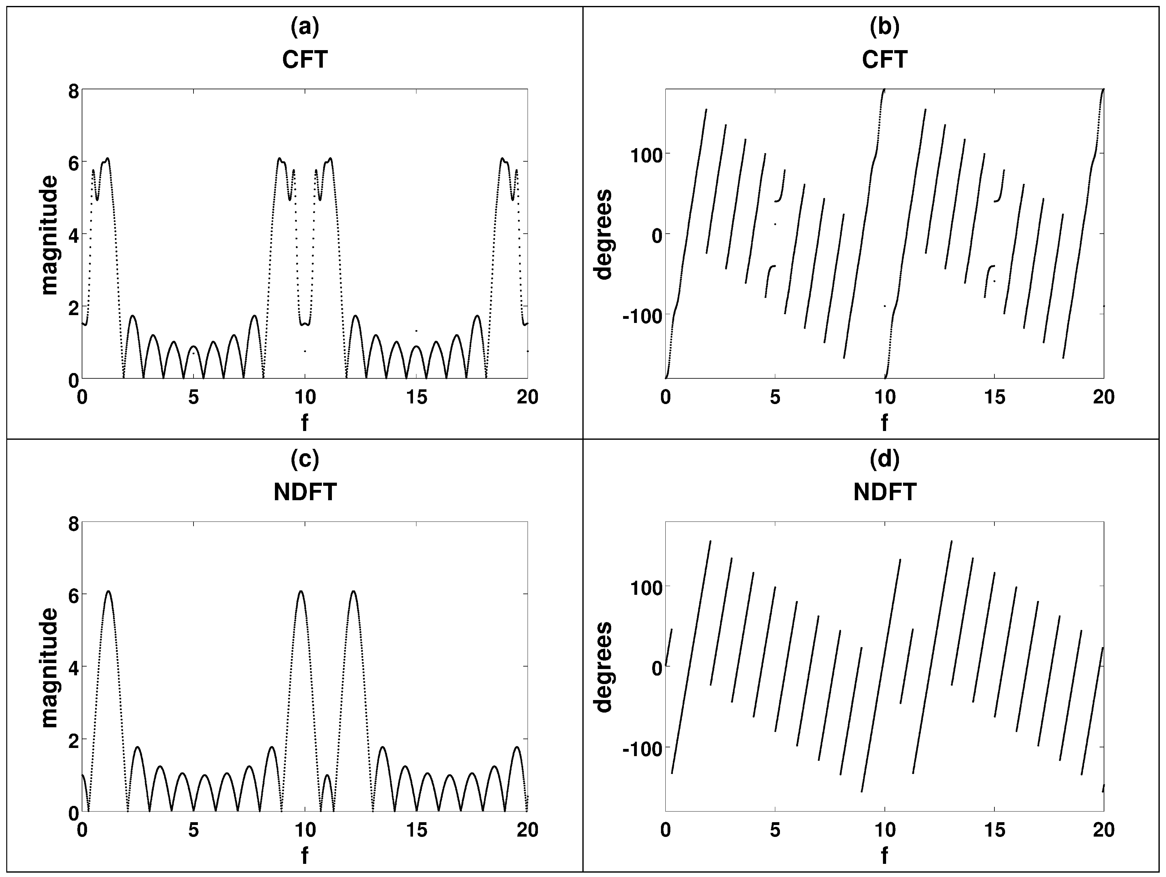
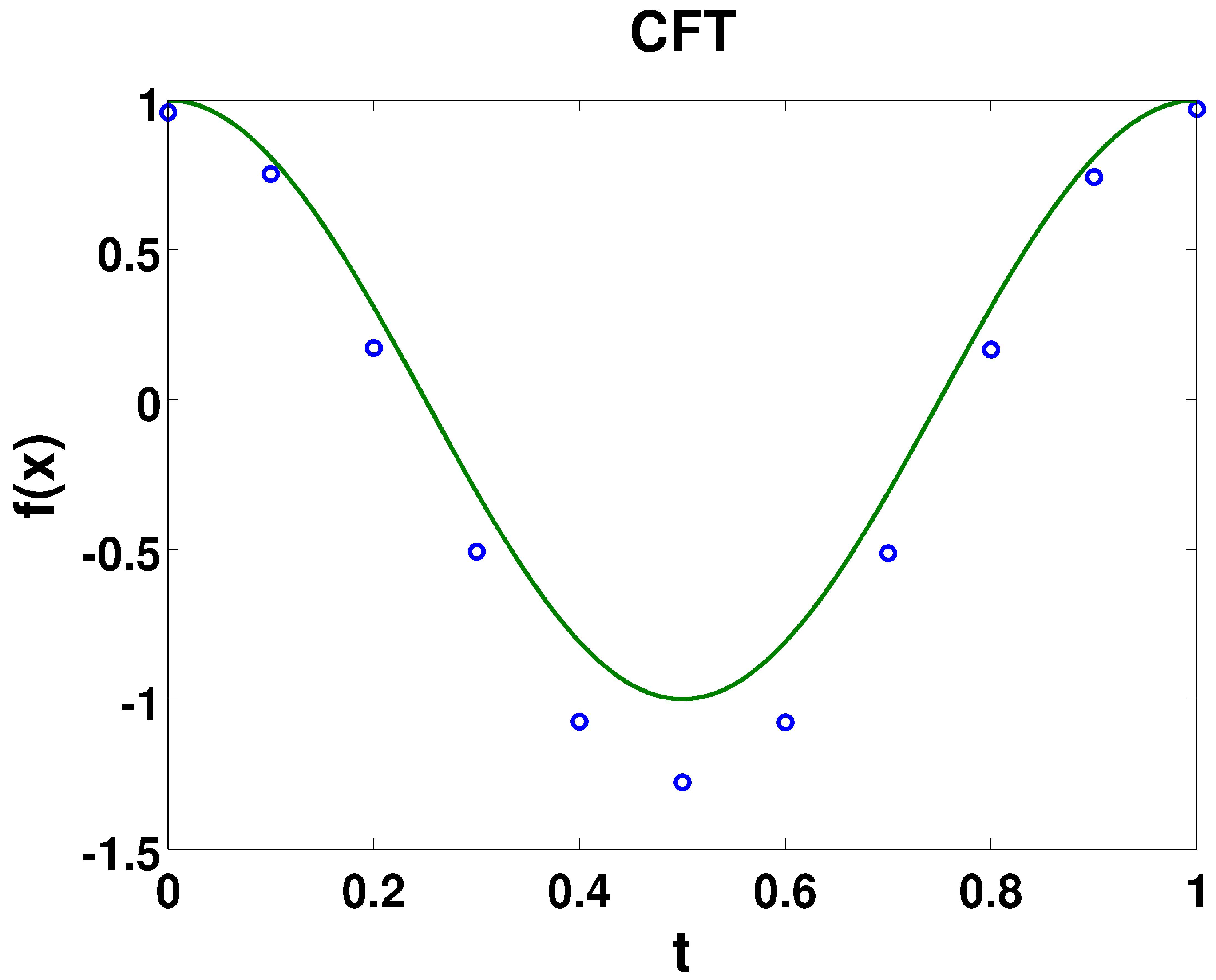
The spectral transform was taken of all six of these functions with both the CFT algorithm, as well as the NDFT algorithm defined in Equation (6). The spectral magnitude and phase from both methods are plotted in Figure 2. By using Equation (12) to get back to the temporal domain (one example is plotted in Figure 3), all six functions matched ( > 0.996) with the spectral magnitude and phase from the CFT; there is no coherent match for the NDFT. This is realized by finding the coefficient of determination between the recovered temporal data and the original temporal data; the results are tabulated in Table 2. While the NDFT may give a clear picture of the spectral domain of the function, it is impossible to recover the function back to the original temporal domain without excessively computationally intensive matrix analysis. The strength of CFT transform lies in its inverse operator defined in Equation (12), with which the true temporal function can be obtained back from the spectral domain obtained with highly resolved CFT.
One important point is that, while the CFT transform is a spectral representation of the transformed temporal function, the spectral function of this method is not a true Fourier transform defined analytically in Equation (1). Both functions are similar (see Figure 2), but not exact; this function, by definition, is the magnitude of the coefficient of determination of the temporal function with the associated sine and cosine wave. For this reason, the CFT versions of the spectral representation, while similar, are not identical to the NDFT versions, and thus are not true Fourier transforms. The power of these CFT spectral plots lie in the fact that they can be easily transformed back to the temporal domain.
5. Performance of the Spectral Transform Algorithm
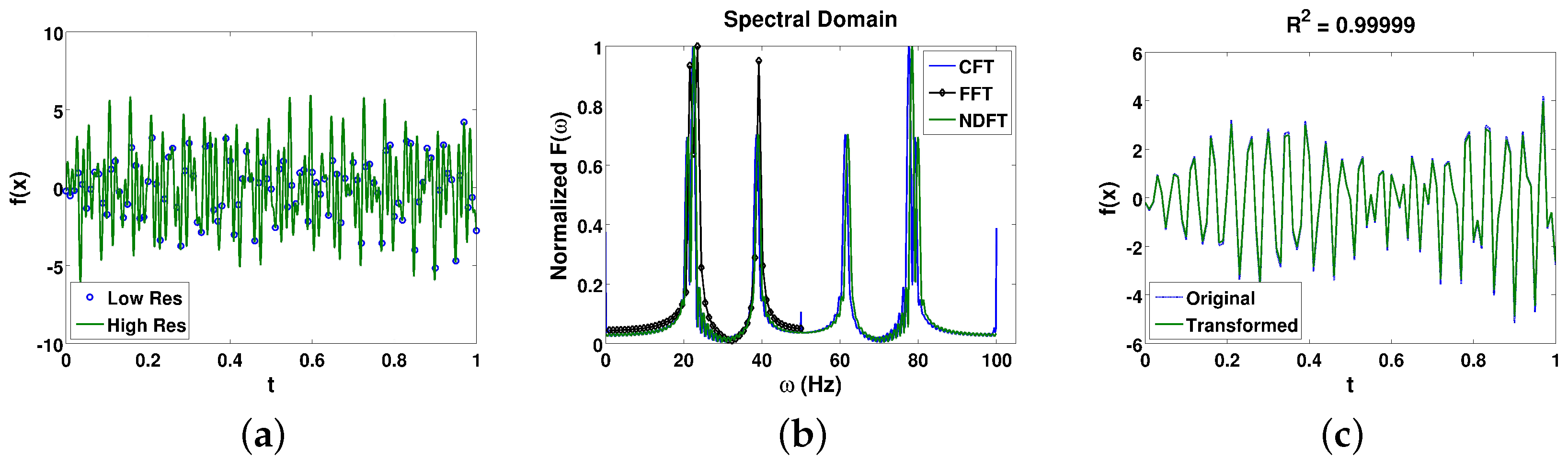
In the previous sections, this algorithm was demonstrated to be an effective tool to determine spectral magnitude and phase. Next, this algorithm’s performance was compared to both traditional FFT [11,12] of limited resolution, as well as the higher resolution NDFT method [23,24,25,26,27,28,29,30,31]. Often in practical applications it is necessary to determine the frequencies of the peak spectral magnitudes with temporal data of limited resolution. In this example, a temporal function is comprised of four sinusoidal functions with an amplitude of 1.25, 1.5, 1.75, and 2, at frequencies of 20.80 Hz, 38.38 Hz, 61.38 Hz, and 77.55 Hz, at a phase shift of 0, 120, 240, and 0, respectively. Mathematically, the function can be described as
The function is performed over a temporal duration of 1 unit of time. The function is plotted in Figure 4a, where the green lines represent the highly resolved function, and the blue circles represent the limited temporal data of 100 Hz one might practically receive if collecting experimental data.
A traditional FFT of this limited-resolution temporal data was collected, along with a CFT with a spectral domain of 0.01 Hz ranging from 0.01 Hz to 100 Hz, as well as a NDFT transform with the same refined spectral domain; the spectral magnitudes are all plotted in Figure 4b. The peak spectral magnitudes were numerically found in the spectral range of 10–30 Hz, 30–50 Hz, 50–70 Hz, and 70–90 Hz, and tabulated in Table 3. For all four frequencies, the CFT improved upon traditional FFT in terms of accurately centering on the frequency with peak spectral magnitude. In addition, with limited resolution tradition FFT cannot even characterize frequencies higher than half the resolution (Equation (5)); the spectral plots are limited up to 50 Hz. The NDFT method with the higher resolution allowed for spectral characterization above 50 Hz, and improved upon the accuracy of the spectral peaks when compared to the traditional FFT, but still with greater error than the CFT. In addition, the CFT results can be accurately transformed back to the temporal domain with Equation (12), and in this case the transform of the spectral results matched remarkably (R = 0.99999) with the original temporal function, as demonstrated in Figure 4c.
6. Parametric Study of the Spectral Transform Algorithm
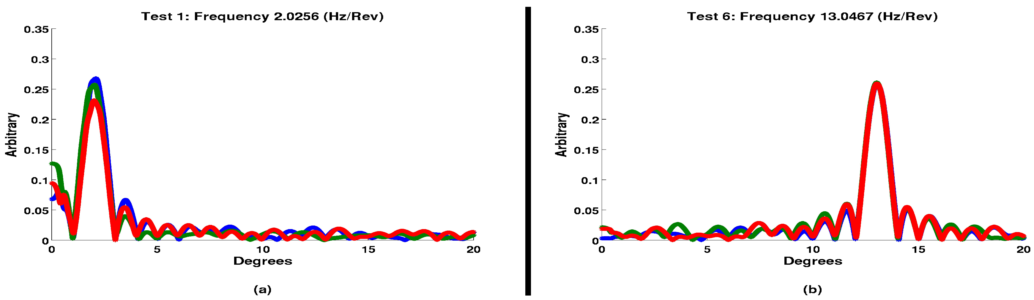
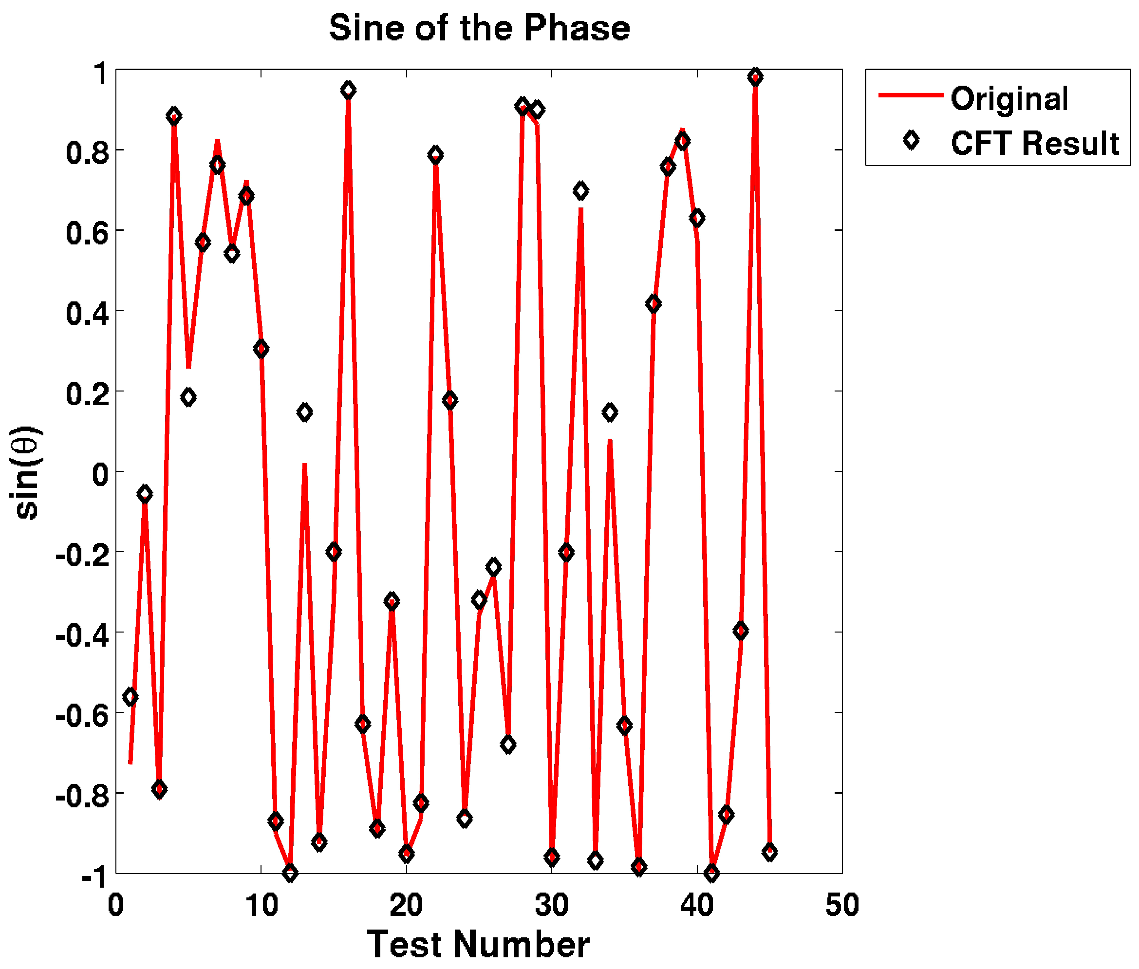
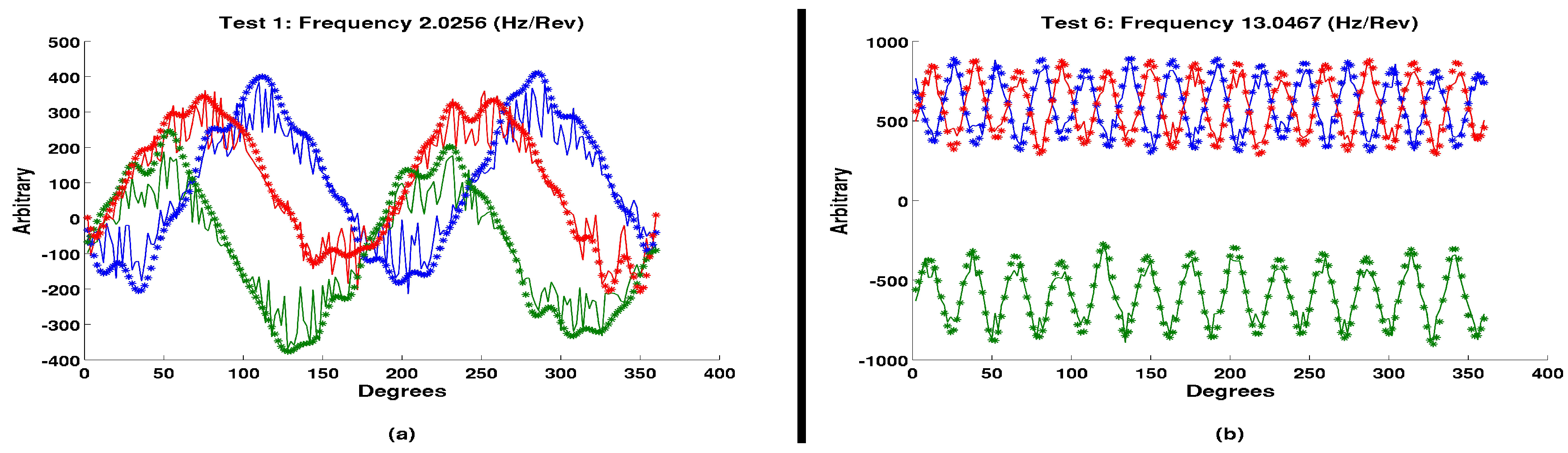
A parametric study of this transform was conducted to demonstrate that it can be used for high resolution measurements of the spectral frequency with a limited temporal resolution. To demonstrate this, 15 random frequencies were selected, ranging from 2 to 17 cycles over the duration of the measured window. Both the independent and dependent temporal variables are arbitrary values to demonstrate the transform function; the independent scale ranges from 0 to 1 and has 180 data points. The arbitrary dependent data had random averages between −1000 and 1000, with an amplitude of 200 and random noise to represent the typical randomness found in typical test data. Each of these 15 random frequencies was phase shifted by three random phases. All forty-five arbitrary functions were transformed into the spectral domain with this transform, with a frequency domain ranging from 0 to 20 cycles per unit time duration, and a frequency resolution of 1 mHz; two examples of these spectral results are presented in Figure 5. As a further test of the robustness of the transform, the spectral data were then converted back to the temporal domain, and the new temporal function was compared to the original function with the coefficient of determination method to ascertain errors from the transform.
This spectral transform was remarkably effective at finding the peak primary frequency, often with accuracies down to tens of mHz. The functions of the peak frequencies (Figure 6), both of which were used for the initial function and the peak of the spectral transform, match with an value of 0.999991—effectively identical. The functions of the random phase angle at the peak frequencies (Figure 7), both of which were used for the initial function and the phase of the spectral transform at the peak frequency, match with an value of 0.9982, demonstrating that this transform can be used to capture both spectral magnitude and phase with great accuracy.
Finally, the inverse of this spectral transform was conducted for each spectral output, and the errors between the original functions and the transformed-inverse-transformed function are minimal. As expected, not all of the fine random noise is captured; this would require a near infinite spectral domain, which would further increase computational costs, but the overarching shapes, magnitudes, and phases of the functions are consistently captured. Taking the coefficient of determination of each function pair, the value of is never less than 0.92. Two examples of the original function (lines) and the transformed-inverse-transformed function (stars) are represented in Figure 8. The tabulated results of all fifteen studies, for each of the three phase magnitude shifts, are demonstrated in Table 4, Table 5 and Table 6.
7. Conclusions
This effort has demonstrated a practical, working, invertible method of numerically transforming a 1D temporal function, called Coefficient of determination Fourier Transform(CFT), obtaining high-resolution in the spectral domain from limited resolution in the temporal domain, and retaining the ability to go back to the temporal domain from the spectral data with Equation (12). The CFT algorithm, while very similar, is not a true Fourier transform as defined analytically in Equation (1); it is a representation of the spectral magnitudes as related to its coefficient of determination value. The CFT transform inherently is more computationally expensive than traditional DFT and NDFT methods. Any desired spectral resolution and spectral domain can be used to characterize the input data. The transform can even convert the function to a spectral domain of varying resolution, so that peaks can be accurately identified without too much computational expense. The algorithm was first tested with simple phase-shifted cosine functions, and the inverse transform of the spectral resolution matched remarkably. Next, the spectral transform algorithm was tested at fifteen different random frequencies, all with three different random phases, all with random noises and errors, and consistently the transform was able to characterize the peak frequency and phase angle remarkably, with a higher degree of accuracy than one can expect with traditional DFT methods.
Supplementary Materials
The following are available online at https://0-www-mdpi-com.brum.beds.ac.uk/2079-3197/6/4/61/s1, Run_Initial_Study.zip.
Funding
This research received no external funding.
Acknowledgments
The author would like to acknowledge Lou Vocaturo and Kevin Larkins for useful discussions.
Conflicts of Interest
The founding sponsors had no role in the design of the study; in the collection, analyses, or interpretation of data; in the writing of the manuscript, and in the decision to publish the results.
Abbreviations
The following abbreviations are used in this manuscript:
| MDPI | Multidisciplinary Digital Publishing Institute |
| DOAJ | Directory of open access journals |
| DFT | Discrete Fourier Transform |
| FFT | Fast Fourier Transform |
| NDFT | Non-uniform Discrete Fourier Transform |
| CFT | Coefficient of determination Fourier Transform |
| Generic temporal function of time t. | |
| F() | Generic spectral function of frequency . |
| a discrete spectral value of the frequency | |
| a discrete temporal value of the time domain | |
| a discrete value of the temporal function | |
| arbitrary temporal resolution for NDFT | |
| (t) | Cosine function to represent real discrete spectral magnitude as related to (Equation (7)) |
| (t) | Sine function to represent imaginary discrete spectral magnitude (Equation (7)) |
| A | Amplitude of functions (t) and (t) (Equation (8)) |
| arbitrary function of discrete temporal value . is the mean of . | |
| arbitrary function of discrete temporal value . is the mean of . |
References
- Nagel, R.K.; Saff, E.B.; Snider, A.D. Fundamentals of Differential Equations, 5th ed.; Addison Wesley: Boston, MA, USA, 1999. [Google Scholar]
- Haberman, R. Applied Partial Differential Equations with Fourier Series and Boundary Value Problems, 4th ed.; Prentice Hall: Upper Saddle River, NJ, USA, 2003. [Google Scholar]
- Harris, F.J. On the Use of Windows for Harmonic Analysis with the Discrete Fourier Transform. Proc. IEEE 1978, 66, 51–83. [Google Scholar] [CrossRef]
- Dorrer, C.; Belabas, N.; Likforman, J.P.; Joffre, M. Spectral resolution and sampling issues in Fourier-transform spectral interferometry. J. Opt. Soc. Am. B 2000, 17, 1795–1802. [Google Scholar] [CrossRef]
- Arfken, G.B.; Weber, H.J. Mathematical Methods for Physicists, 6th ed.; Elsevier: Burlington, MA, USA, 2005. [Google Scholar]
- Zill, D.G.; Cullen, M.R. Advanced Engineering Mathematics, 2nd ed.; Jones and Bartlett Publishers: Sudbury, MA, USA, 2000. [Google Scholar]
- Numerical Recipies in C: The Art of Scientific Computing; Cambridge University Press: Cambridge, UK, 1988; Chapter 13; pp. 584–591. ISBN 0-521-4310805.
- Chen, W.H.; Smith, C.H.; Fralick, S.C. A Fast Computational Algorithm for the Discrete Cosine Transform. IEEE Trans. Commun. 1977, 25, 1004–1009. [Google Scholar] [CrossRef]
- Agarwal, R.C. A New Least-Squares Refinement Technique Based on the Fast Fourier Transform Algorithm. Acta Cryst. 1978, 34, 791–809. [Google Scholar] [CrossRef]
- Finzel, B. Incorporation of fast Fourier transforms to speed restrained least-squares refinement of protein structures. J. Appl. Cryst. 1986, 20, 53–55. [Google Scholar] [CrossRef]
- Garcia, A. Numerical Methods for Physics, 2nd ed.; Addison-Wesley: Boston, MA, USA, 1999. [Google Scholar]
- Poon, T.C.; Kim, T. Engineering Optics With Matlab; World Scientific Publishing Co.: Hackensack, NJ, USA, 2006. [Google Scholar]
- Nyquist, H. Certain Topics in Telegraph Transmission Theory. Proc. IEEE 2002, 90, 280–305. [Google Scholar] [CrossRef]
- Landau, H.J. Necessary Density Conditions for Sampling and Interpolation of Certain Entire Functions. Acta Math. 1967, 117, 37–52. [Google Scholar] [CrossRef]
- Shannon, C.E. Communication in the Presence of Noise. Proc. IEEE 1998, 86, 447–457. [Google Scholar] [CrossRef]
- Luke, H.D. The Origins of the Sampling Theorem. IEEE Commun. Mag. 1999, 37, 106–108. [Google Scholar] [CrossRef]
- Kupfmuller, K. On the Dynamics of Automatic Gain Controllers. Elektr. Nachrichtentech. 2005, 5, 459–467. [Google Scholar]
- Harvey, J. Fourier treatment of near-field scalar diffraction theory. Am. J. Phys. 1979, 47, 974–980. [Google Scholar] [CrossRef]
- Jiang, D.; Stamnes, J.J. Numerical and experimental results for focusing of two-dimensional electromagnetic waves into uniaxial crystals. Opt. Commun. 2000, 174, 321–334. [Google Scholar] [CrossRef]
- Stamnes, J.J.; Jiang, D. Focusing of electromagnetic waves into a uniaxial crystal. Opt. Commun. 1998, 150, 251–262. [Google Scholar] [CrossRef]
- Jiang, D.; Stamnes, J.J. Numerical and asymptotic results for focusing of two-dimensional waves in uniaxial crystals. Opt. Commun. 1999, 163, 55–71. [Google Scholar] [CrossRef]
- Shen, F.; Wang, A. Fast-Fourier-transform based numerical integration method for the Rayleigh–Sommerfeld diffraction formula. Appl. Opt. 2006, 45, 1102–1110. [Google Scholar] [CrossRef] [PubMed]
- Boyd, J.P. A Fast Algorithm for Chebyshev, Fourier, and Sine Interpolation onto an Irregular Grid. J. Comput. Phys. 1992, 103, 243–257. [Google Scholar] [CrossRef]
- Lee, J.Y.; Greengard, L. The type 3 nonuniform FFT and its applications. J. Comput. Phys. 2005, 206, 1–5. [Google Scholar] [CrossRef]
- Dutt, A. Fast Fourier Transforms for Nonequispaced Data. Ph.D. Thesis, Yale University, New Haven, CT, USA, 1993. [Google Scholar]
- Dutt, A.; Rokhlin, V. Fast Fourier Transforms for Nonequispaced Data II. SIAM J. Sci. Ccomput. 1993, 14, 1368–1393. [Google Scholar] [CrossRef]
- Dutt, A.; Rokhlin, V. Fast Fourier Transforms for Nonequispaced Data II. Appl. Comput. Harmon. Anal. 1995, 2, 85–100. [Google Scholar] [CrossRef]
- Greengard, L.; Lee, J.Y. Accelerating the Nonuniform Fast Fourier Transform. SIAM Rev. 2004, 46, 443–454. [Google Scholar] [CrossRef] [Green Version]
- Dohler, M.; Kunis, S.; Potts, D. Nonequispaced Hyperbolic Cross Fast Fourier Transform. SIAM J. Numer. Anal. 2010, 47, 4415–4428. [Google Scholar] [CrossRef] [Green Version]
- Fessler, J.A.; Sutton, B.P. Nonuniform Fast Fourier Transforms Using Min-Max Interpolation. IEEE Trans. Signal Process. 2003, 51, 560–574. [Google Scholar] [CrossRef]
- Ruiz-Antolin, D.; Townsend, A. A Nonuniform Fast Fourier Transform Based on Low Rank Approximation. SIAM J. Sci. Comput. 2018, 40, 529–547. [Google Scholar] [CrossRef]
- Cameron, A.C.; Windmeijer, F.A. An R-squared measure of goodness of fit for some common nonlinear regression models. J. Econ. 1997, 77, 329–342. [Google Scholar] [CrossRef]
- Magee, L. R2 Measures Based on Wald and Likelihood Ratio Joint Significance Tests. Am. Stat. 1990, 44, 250–253. [Google Scholar]
- Nagelkerke, N.J.D. A note on a general definition of the coefficient of determination. Biomelrika 1991, 78, 691–692. [Google Scholar] [CrossRef]
- Strang, G. Introduction to Linear Algebra, 3rd ed.; Wellesley-Cambridge Press: Wellesley, MA, USA, 2003. [Google Scholar]
Figure 1.
Equal values for f = 1 and f = 9 for .

Figure 2.
Spectral results of the function with a s = 0.1, with both the proposed CFT in magnitude (a) and phase (b), as well as NDFT in magnitude (c) and phase (d).
Figure 2.
Spectral results of the function with a s = 0.1, with both the proposed CFT in magnitude (a) and phase (b), as well as NDFT in magnitude (c) and phase (d).

Figure 3.
Demonstration of the function , both the original function (solid green lines), and the output (blue circles) obtained from Equation (12) and the CFT spectral results, obtained with a limited initial temporal resolution of .
Figure 3.
Demonstration of the function , both the original function (solid green lines), and the output (blue circles) obtained from Equation (12) and the CFT spectral results, obtained with a limited initial temporal resolution of .

Figure 4.
Performance data for an input temporal plot of 101 data points of resolution: (a) a comparison of the data to the true, high resolution function; (b) the spectral function, both the CFT and a tradition FFT analysis; and (c) the original versus the inverse transform of the spectral function.

Figure 5.
Spectral results of the randomly generated functions, for frequencies of: (a) 2.0256 (Hz/Rev); and (b) 13.0467 (Hz/Rev), but for different phases, magnitudes, and random noises.
Figure 5.
Spectral results of the randomly generated functions, for frequencies of: (a) 2.0256 (Hz/Rev); and (b) 13.0467 (Hz/Rev), but for different phases, magnitudes, and random noises.

Figure 6.
Frequency prediction results, .
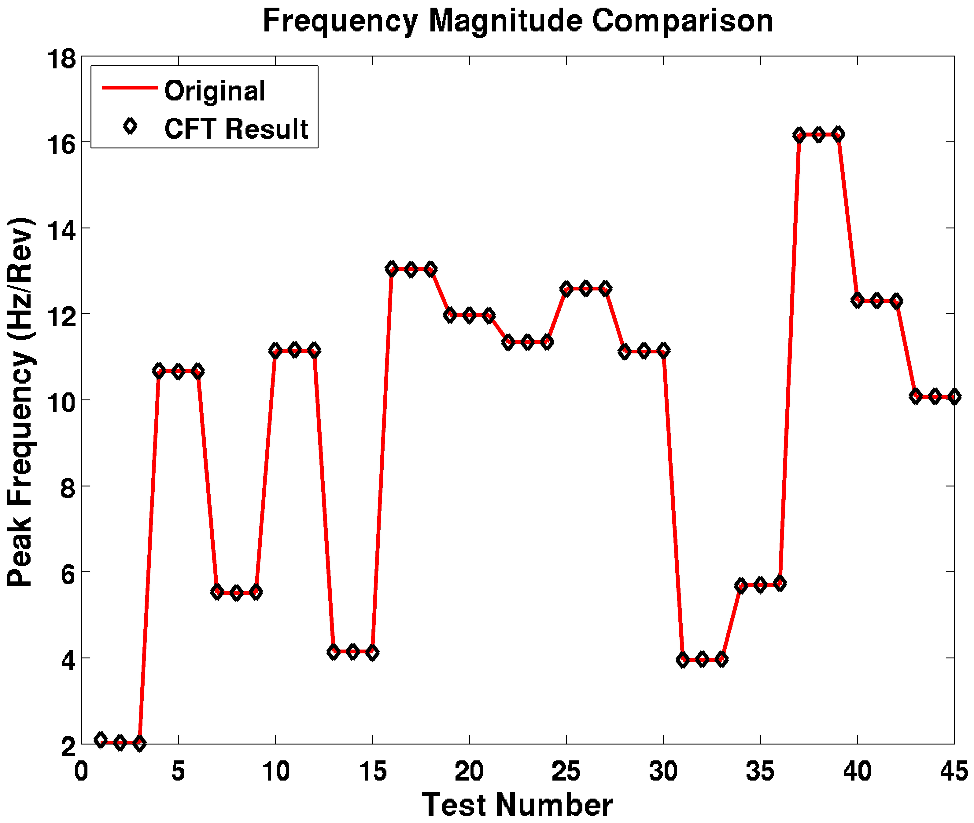
Figure 7.
Angle prediction results, .

Figure 8.
Time results of the randomly generated functions, for frequencies of: (a) 2.0256 (Hz/Rev); and (b) 13.0467 (Hz/Rev), but for different phases, magnitudes, and random noises.
Figure 8.
Time results of the randomly generated functions, for frequencies of: (a) 2.0256 (Hz/Rev); and (b) 13.0467 (Hz/Rev), but for different phases, magnitudes, and random noises.


Table 1.
Equal values for f = 1 and f = 9 for .
| x | f = 1 | f = 9 |
|---|---|---|
| 0.0 | 1.0000 | 1.0000 |
| 0.1 | 0.8090 | 0.8090 |
| 0.2 | 0.3090 | 0.3090 |
| 0.3 | −0.3090 | −0.3090 |
| 0.4 | −0.8090 | −0.8090 |
| 0.5 | −1.0000 | −1.0000 |
| 0.6 | −0.8090 | −0.8090 |
| 0.7 | −0.3090 | −0.3090 |
| 0.8 | 0.3090 | 0.3090 |
| 0.9 | 0.8090 | 0.8090 |
| 1.0 | 1.0000 | 1.0000 |
Table 2.
Coefficient of determination between the original temporal function and the temporal function retrieved (Equation (12)) from the spectral plot obtained with both CFT and NDFT (Figure 2).
| f (Hz) | Phase | CFT | NDFT |
|---|---|---|---|
| 1 | 0 | 0.9999 | 0.1197 |
| ine 1 | 2/3 | 0.9967 | 0.0091 |
| 1 | /3 | 0.9964 | 0.0163 |
| ine 9 | 0 | 0.9999 | 0.1197 |
| 9 | 2/3 | 0.9964 | 0.0163 |
| 9 | /3 | 0.9967 | 0.0091 |
Table 3.
Performance results of peak frequency, comparing CFT versus FFT, with a temporal resolution of 101.
Table 3.
Performance results of peak frequency, comparing CFT versus FFT, with a temporal resolution of 101.
| True Frequency (Hz) | CFT Frequency (Hz) | FFT Frequency (Hz) | NDFT Frequency (Hz) |
|---|---|---|---|
| 20.8 | 22.42 | 23.5294 | 22.63 |
| 38.38 | 38.58 | 39.2157 | 38.98 |
| 61.38 | 61.42 | - | 62.02 |
| 77.55 | 77.58 | - | 78.37 |
Table 4.
Comparison of results, for phase shift angle 1.
| Test | Max Freq | Max Freq | Sin(Phase) | Sin(Phase) | |
|---|---|---|---|---|---|
| Original | CFT Result | Original | CFT Result | (Temporal) | |
| 1 | 2.0256 | 2.095 | −0.72837 | −0.56129 | 0.92791 |
| 2 | 10.6771 | 10.678 | 0.88707 | 0.88349 | 0.94843 |
| 3 | 5.5118 | 5.537 | 0.82648 | 0.76277 | 0.94092 |
| 4 | 11.1441 | 11.146 | 0.32585 | 0.30499 | 0.93117 |
| 5 | 4.1527 | 4.137 | 0.020562 | 0.14696 | 0.93132 |
| 6 | 13.0467 | 13.05 | 0.94015 | 0.94829 | 0.93359 |
| 7 | 11.9742 | 11.973 | −0.31888 | −0.32338 | 0.92769 |
| 8 | 11.3472 | 11.339 | 0.78318 | 0.78725 | 0.93398 |
| 9 | 12.5892 | 12.578 | −0.35645 | −0.31945 | 0.93956 |
| 10 | 11.128 | 11.122 | 0.90871 | 0.90812 | 0.92836 |
| 11 | 3.9531 | 3.954 | −0.20131 | −0.20166 | 0.93636 |
| 12 | 5.6981 | 5.677 | 0.080619 | 0.14678 | 0.93363 |
| 13 | 16.1721 | 16.158 | 0.38625 | 0.41684 | 0.94243 |
| 14 | 12.2989 | 12.32 | 0.57446 | 0.63023 | 0.93483 |
| 15 | 10.0715 | 10.085 | −0.43758 | −0.3967 | 0.92398 |
Table 5.
Comparison of results, for phase shift angle 2.
| Test | Max Freq | Max Freq | Sin(Phase) | Sin(Phase) | |
|---|---|---|---|---|---|
| Original | CFT Result | Original | CFT Result | (Temporal) | |
| 1 | 2.0256 | 2.026 | −0.062681 | 056313 | 0.93311 |
| 2 | 10.6771 | 10.658 | 0.25575 | 0.18466 | 0.93944 |
| 3 | 5.5118 | 5.511 | 0.54959 | 0.54223 | 0.9434 |
| 4 | 11.1441 | 11.166 | 90216 | 87023 | 0.93194 |
| 5 | 4.1527 | 4.141 | 92686 | 92268 | 0.92885 |
| 6 | 13.0467 | 13.031 | 64986 | 6287 | 0.92476 |
| 7 | 11.9742 | 11.97 | 95715 | 95146 | 0.93294 |
| 8 | 11.3472 | 11.344 | 0.16368 | 0.17658 | 0.92725 |
| 9 | 12.5892 | 12.593 | 25732 | 23808 | 0.94473 |
| 10 | 11.128 | 11.145 | 0.86293 | 0.90011 | 0.93841 |
| 11 | 3.9531 | 3.97 | 0.65591 | 0.69795 | 0.94498 |
| 12 | 5.6981 | 5.7 | 62372 | 63233 | 0.93151 |
| 13 | 16.1721 | 16.169 | 0.76013 | 0.75789 | 0.93039 |
| 14 | 12.2989 | 12.31 | 99804 | 0.93751 | |
| 15 | 10.0715 | 10.084 | 0.9865 | 0.98098 | 0.9411 |
Table 6.
Comparison of results, for phase shift angle 3.
| Test | Max Freq | Max Freq | Sin(Phase) | Sin(Phase) | |
|---|---|---|---|---|---|
| Original | CFT Result | Original | CFT Result | (Temporal) | |
| 1 | 2.0256 | 2.009 | 81562 | 79053 | 0.93367 |
| 2 | 10.6771 | 10.666 | 0.58339 | 0.5697 | 0.92987 |
| 3 | 5.5118 | 5.53 | 0.72393 | 0.68535 | 0.93461 |
| 4 | 11.1441 | 11.154 | 99286 | 99909 | 0.92839 |
| 5 | 4.1527 | 4.122 | 3222 | 20013 | 0.95071 |
| 6 | 13.0467 | 13.04 | 90228 | 88856 | 0.94272 |
| 7 | 11.9742 | 11.958 | 86461 | 82531 | 0.93705 |
| 8 | 11.3472 | 11.347 | 85766 | 86378 | 0.93519 |
| 9 | 12.5892 | 12.588 | 66127 | 67959 | 0.92307 |
| 10 | 11.128 | 11.152 | 9832 | 96008 | 0.9276 |
| 11 | 3.9531 | 3.969 | 9574 | 96818 | 0.9428 |
| 12 | 5.6981 | 5.734 | 99907 | 9842 | 0.94156 |
| 13 | 16.1721 | 16.183 | 0.85337 | 0.82142 | 0.93247 |
| 14 | 12.2989 | 12.296 | 86634 | 85394 | 0.92086 |
| 15 | 10.0715 | 10.075 | 94753 | 9473 | 0.94203 |
© 2018 by the author. Licensee MDPI, Basel, Switzerland. This article is an open access article distributed under the terms and conditions of the Creative Commons Attribution (CC BY) license (http://creativecommons.org/licenses/by/4.0/).
Share and Cite
MDPI and ACS Style
Marko, M.D. Coefficient-of-Determination Fourier Transform. Computation 2018, 6, 61. https://0-doi-org.brum.beds.ac.uk/10.3390/computation6040061
AMA Style
Marko MD. Coefficient-of-Determination Fourier Transform. Computation. 2018; 6(4):61. https://0-doi-org.brum.beds.ac.uk/10.3390/computation6040061
Chicago/Turabian StyleMarko, Matthew David. 2018. "Coefficient-of-Determination Fourier Transform" Computation 6, no. 4: 61. https://0-doi-org.brum.beds.ac.uk/10.3390/computation6040061
Note that from the first issue of 2016, this journal uses article numbers instead of page numbers. See further details here.