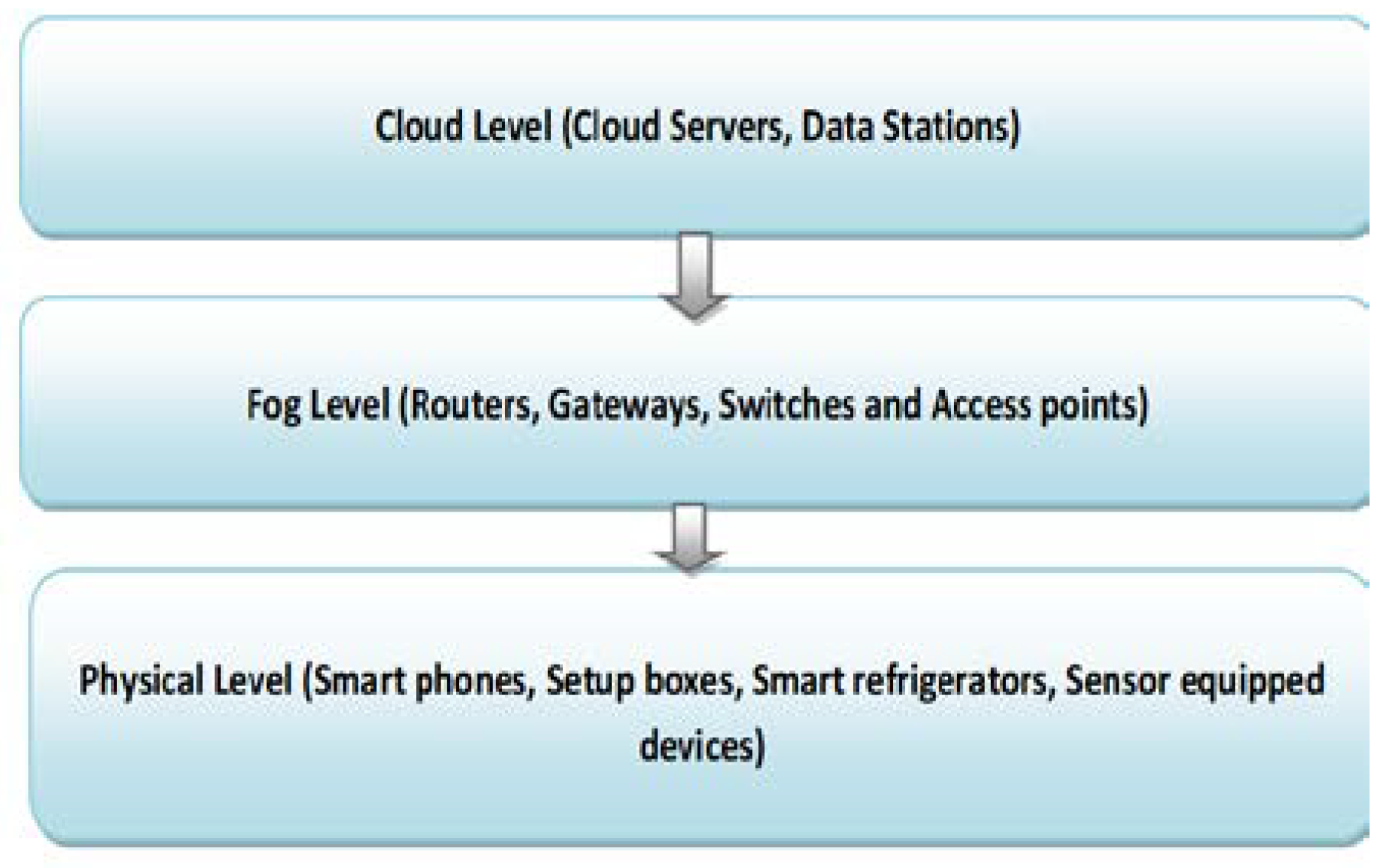
Figure 1.
General three level architecture of fog computing.
Figure 1.
General three level architecture of fog computing.
Figure 2.
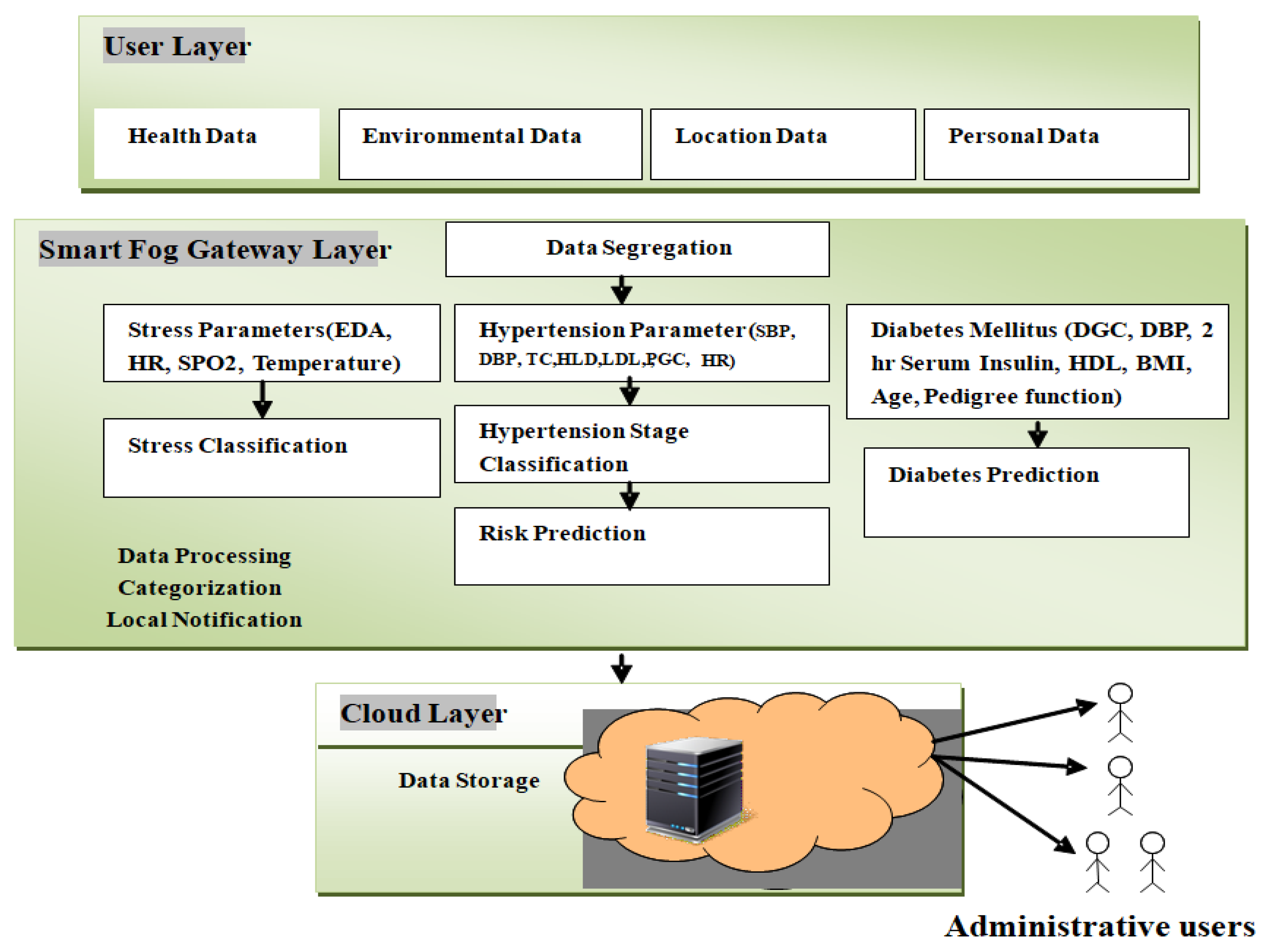
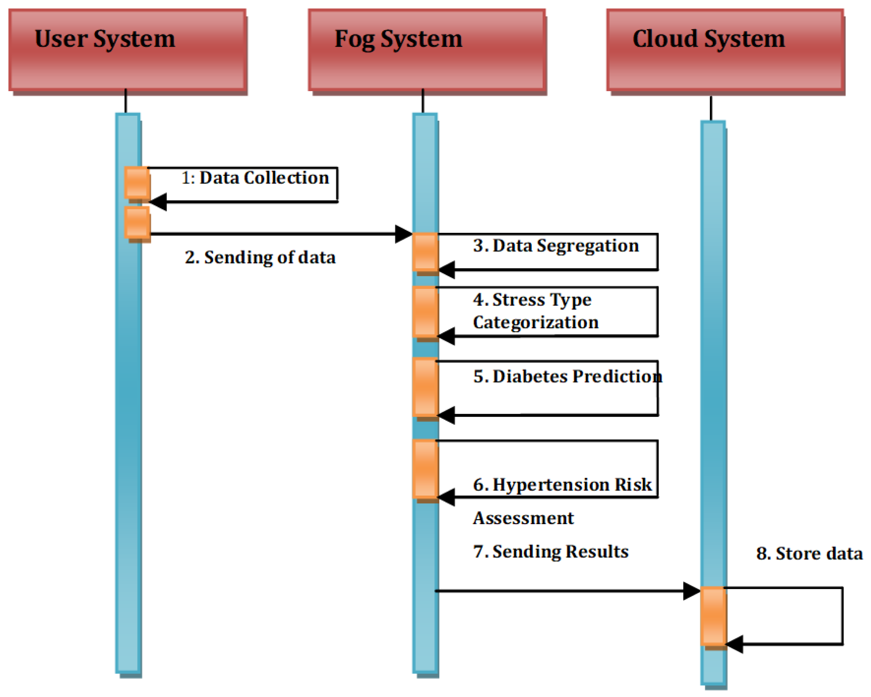
The proposed DeepFog framework has a middle layer that works as a smart gateway, residing between the user and the cloud layer. The user layer is an integration of all smart data capturing devices to collect health-related feature data to diagnose diabetes and hypertension attacks, bio-signals to predict the stress types. Administrative users have access to maintain avariety of datasets stored in the cloud layer.
Figure 2.
The proposed DeepFog framework has a middle layer that works as a smart gateway, residing between the user and the cloud layer. The user layer is an integration of all smart data capturing devices to collect health-related feature data to diagnose diabetes and hypertension attacks, bio-signals to predict the stress types. Administrative users have access to maintain avariety of datasets stored in the cloud layer.
Figure 3.
The proposed System model of the DeepFog.
Figure 3.
The proposed System model of the DeepFog.
Figure 4.
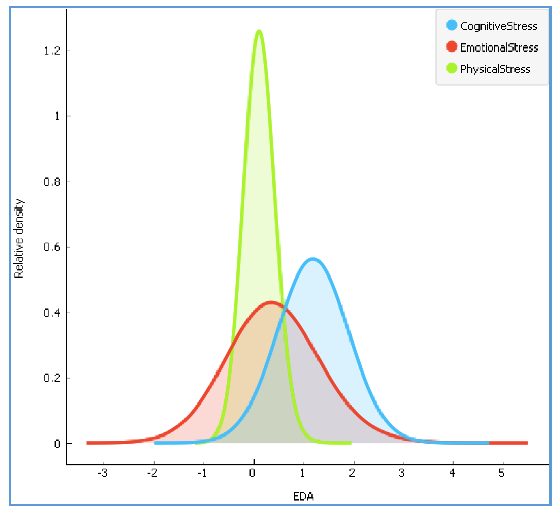
The distribution of according to three stress types.
Figure 4.
The distribution of according to three stress types.
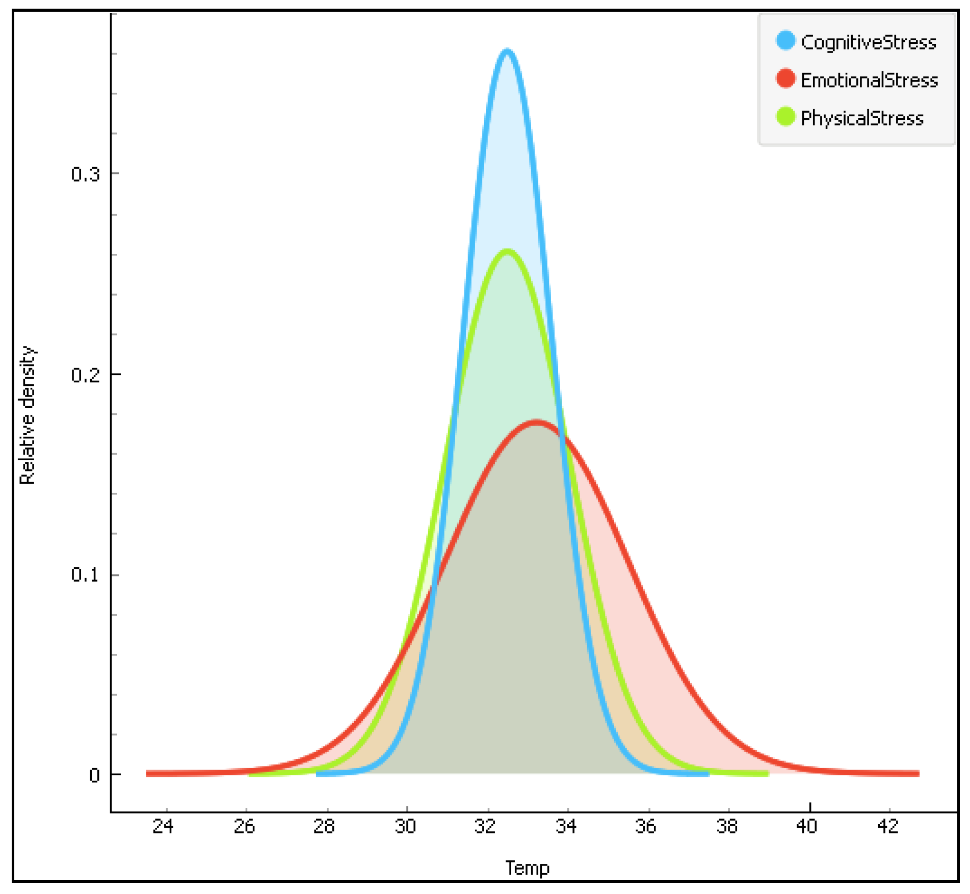
Figure 5.
The distribution of the temperature data(Temp) according to the three stress types.
Figure 5.
The distribution of the temperature data(Temp) according to the three stress types.
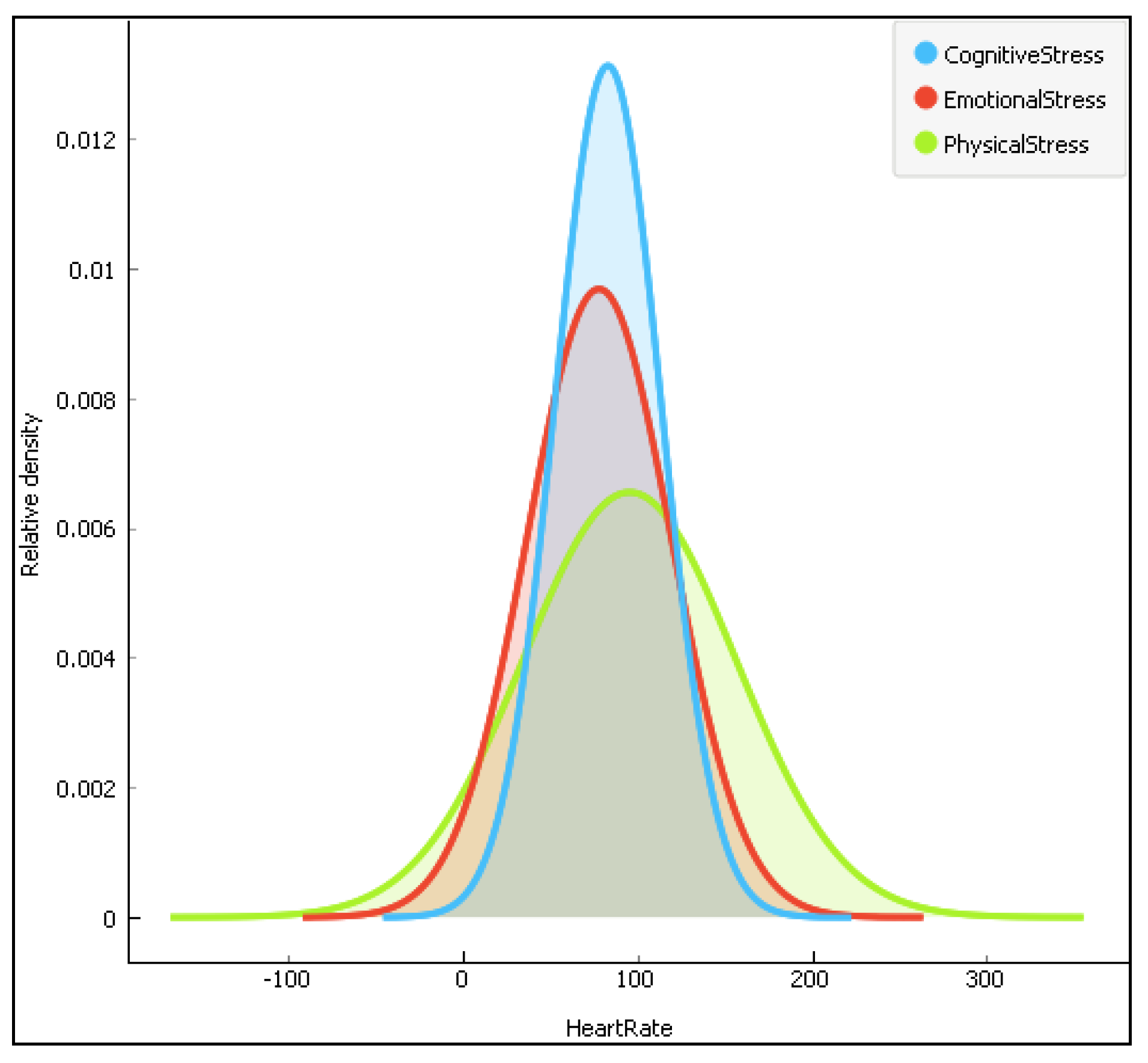
Figure 6.
The distribution of the heartrate data according to the three stress types.
Figure 6.
The distribution of the heartrate data according to the three stress types.
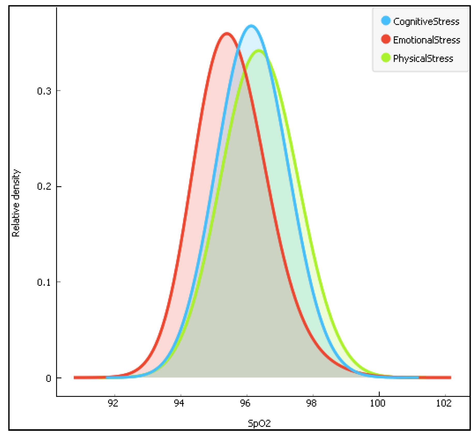
Figure 7.
The distribution of the arterial oxygen saturation data (SpO2) according to the three stress types.
Figure 7.
The distribution of the arterial oxygen saturation data (SpO2) according to the three stress types.
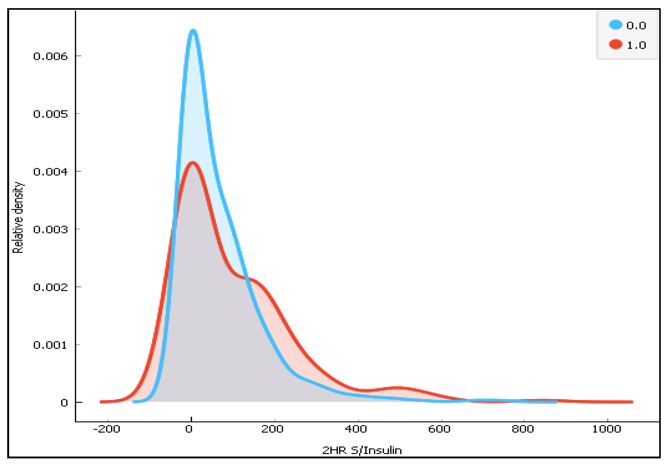
Figure 8.
The distribution of 2-h Serum insulin for the two classes (0-diabetes and 1-non-diabetes).
Figure 8.
The distribution of 2-h Serum insulin for the two classes (0-diabetes and 1-non-diabetes).
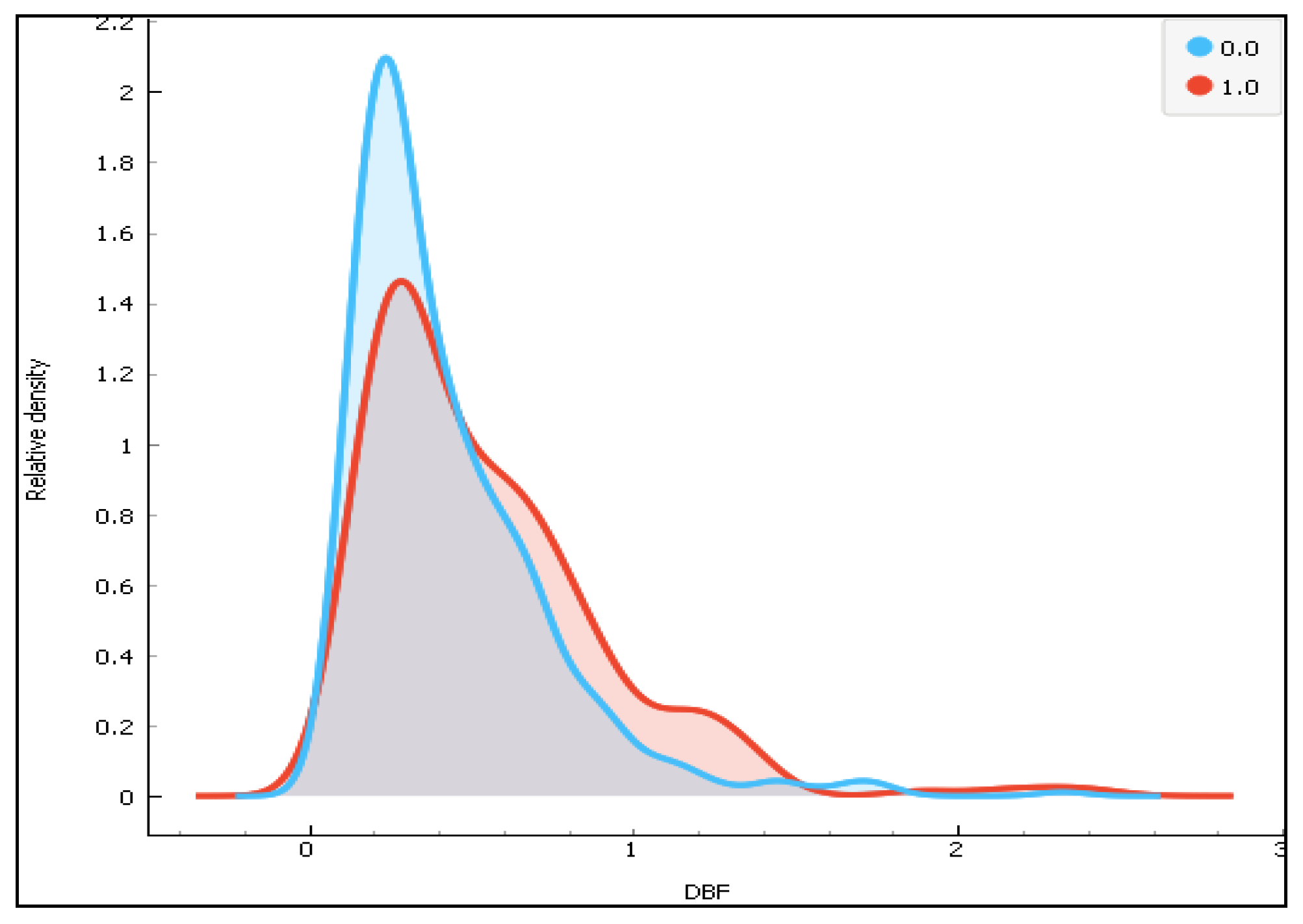
Figure 9.
The distribution of the diabetes pedigree function(DBF) for the two classes.
Figure 9.
The distribution of the diabetes pedigree function(DBF) for the two classes.
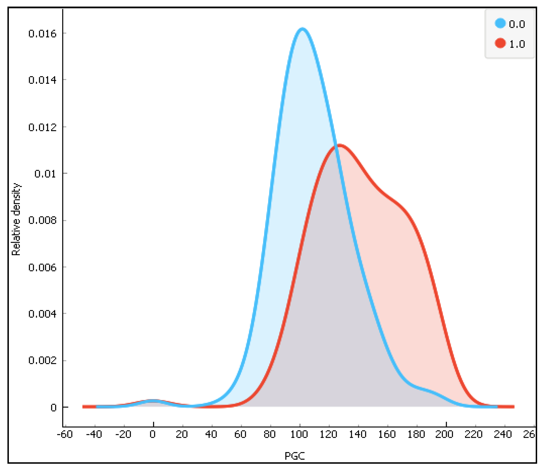
Figure 10.
The distribution of the plasma glucose concentration (PGC) for the two classes (0-diabetes and 1-non-diabetes).
Figure 10.
The distribution of the plasma glucose concentration (PGC) for the two classes (0-diabetes and 1-non-diabetes).
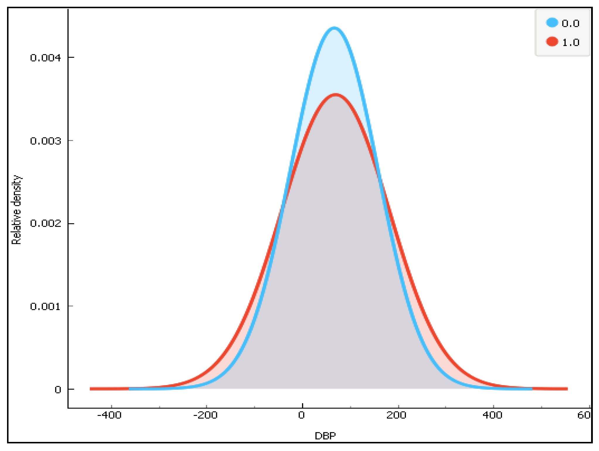
Figure 11.
The distribution of diastolic blood pressure (DBP).
Figure 11.
The distribution of diastolic blood pressure (DBP).
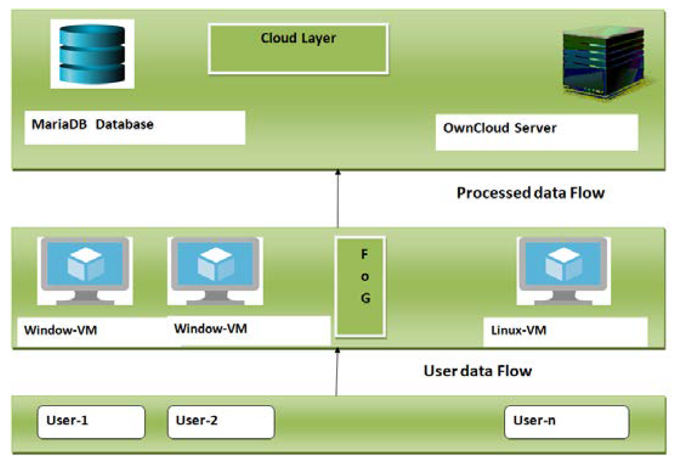
Figure 12.
The fog-based system architecture used to deploy the Deep-fog system.
Figure 12.
The fog-based system architecture used to deploy the Deep-fog system.
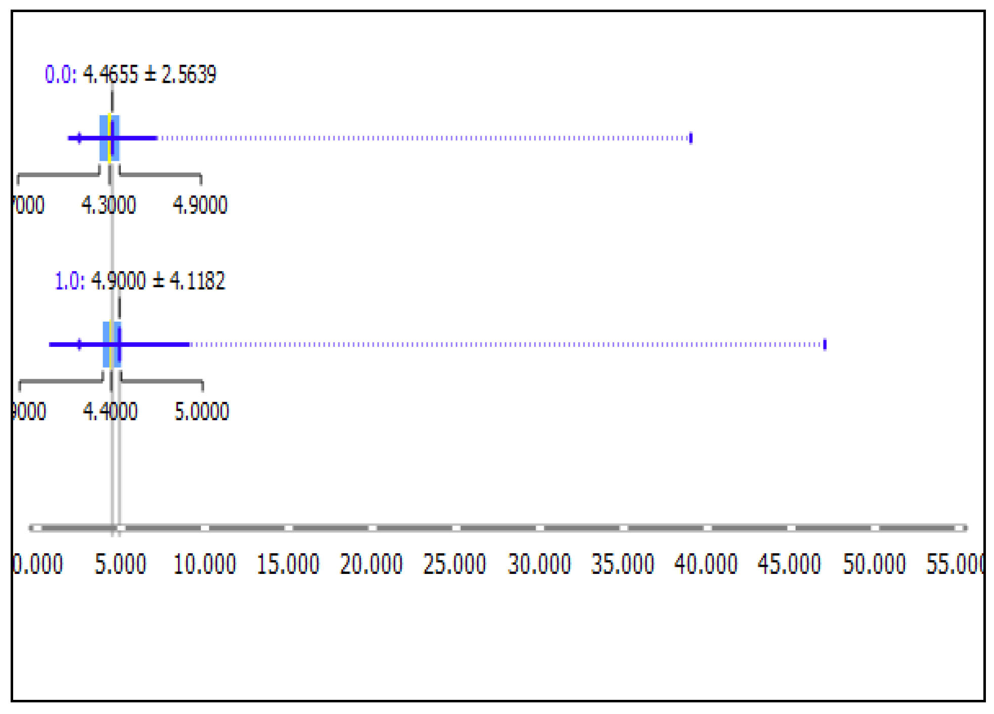
Figure 13.
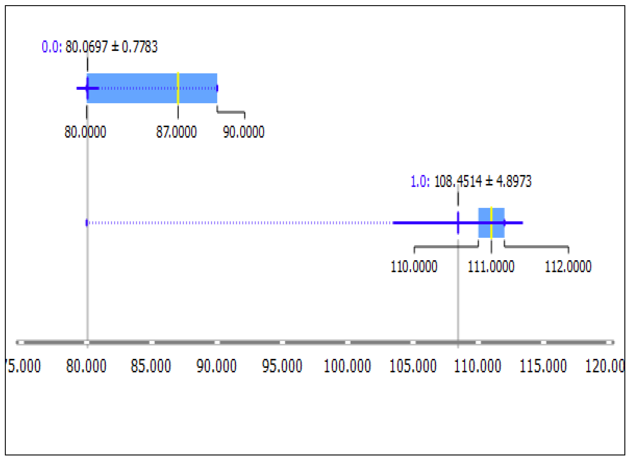
Data distribution of diastolic blood pressure (DBP in a box-plot, showing the range data; the mean value after clustering the data using the K-means clustering technique. Here, 0.0 represents the cluster for the non-hypertension class and 1.0 represents the hypertension class. It can be seen that the two sets of data are non-overlapping in nature.
Figure 13.
Data distribution of diastolic blood pressure (DBP in a box-plot, showing the range data; the mean value after clustering the data using the K-means clustering technique. Here, 0.0 represents the cluster for the non-hypertension class and 1.0 represents the hypertension class. It can be seen that the two sets of data are non-overlapping in nature.
Figure 14.
Data distribution of Systolic Blood Pressure SBP in a box-plot showing the range of the data, its mean value after clustering the data using the K-means clustering technique. Here, 0.0 represents the cluster for the non-hypertension class and 1.0 represents the hypertension class.
Figure 14.
Data distribution of Systolic Blood Pressure SBP in a box-plot showing the range of the data, its mean value after clustering the data using the K-means clustering technique. Here, 0.0 represents the cluster for the non-hypertension class and 1.0 represents the hypertension class.
Figure 15.
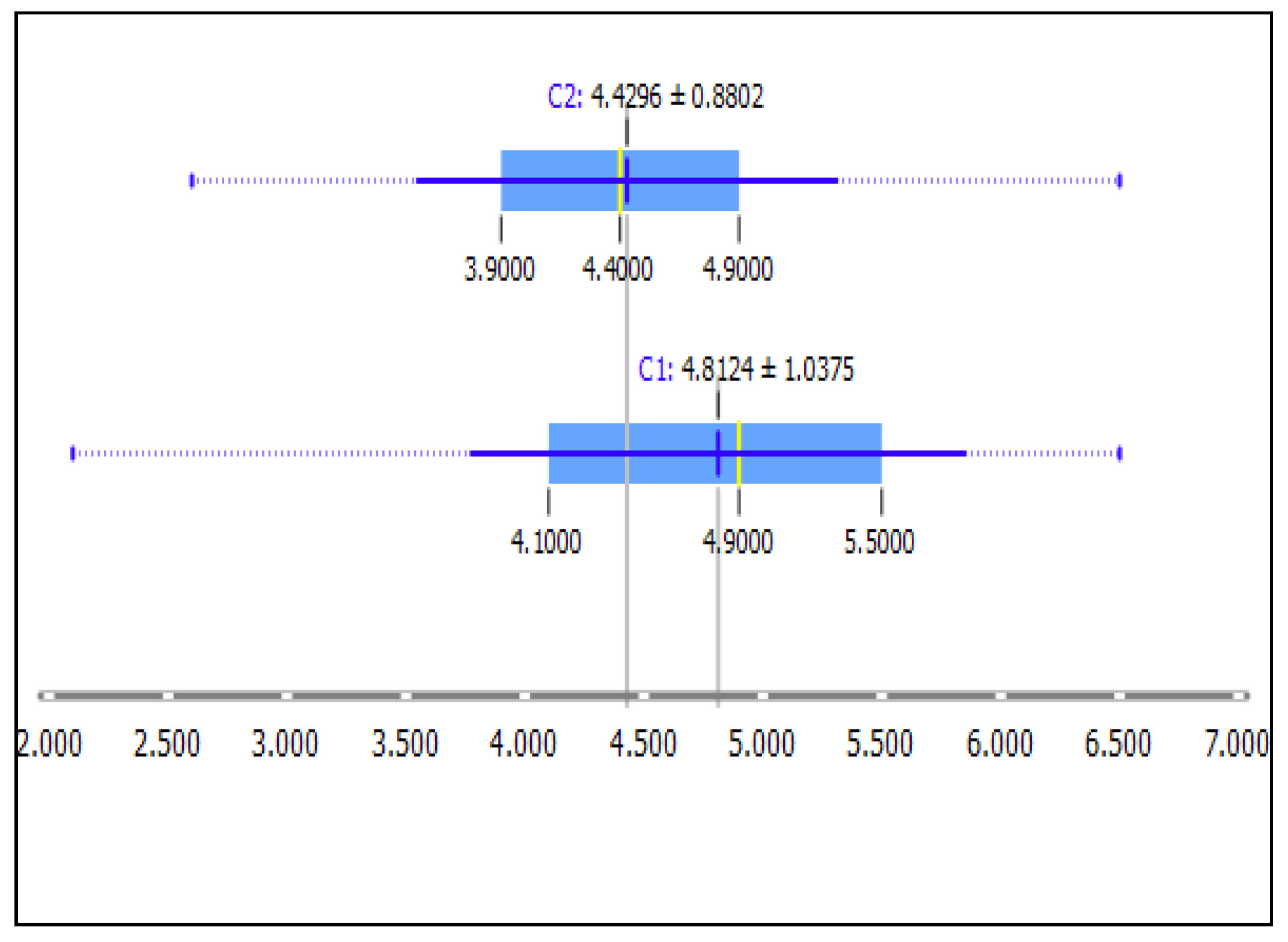
Data distribution of potassium box-plot, showing the range of the data, its mean value after clustering the data using the K-means clustering technique. Here, 0.0 reresents the cluster for the non-hypertension class and 1.0 represents the hypertension class. It can be seen that the two sets of data are overlapping in nature.
Figure 15.
Data distribution of potassium box-plot, showing the range of the data, its mean value after clustering the data using the K-means clustering technique. Here, 0.0 reresents the cluster for the non-hypertension class and 1.0 represents the hypertension class. It can be seen that the two sets of data are overlapping in nature.
Figure 16.
Data distribution of the Red Blood Cell RBC count in a box-plot showing the range of the data, its mean value after clustering the data using the K-means clustering technique. Here, 0.0 reresents the cluster for the non-hypertension class and 1.0 represents the hypertension class. It can be seen that the two sets of data are overlapping in nature.
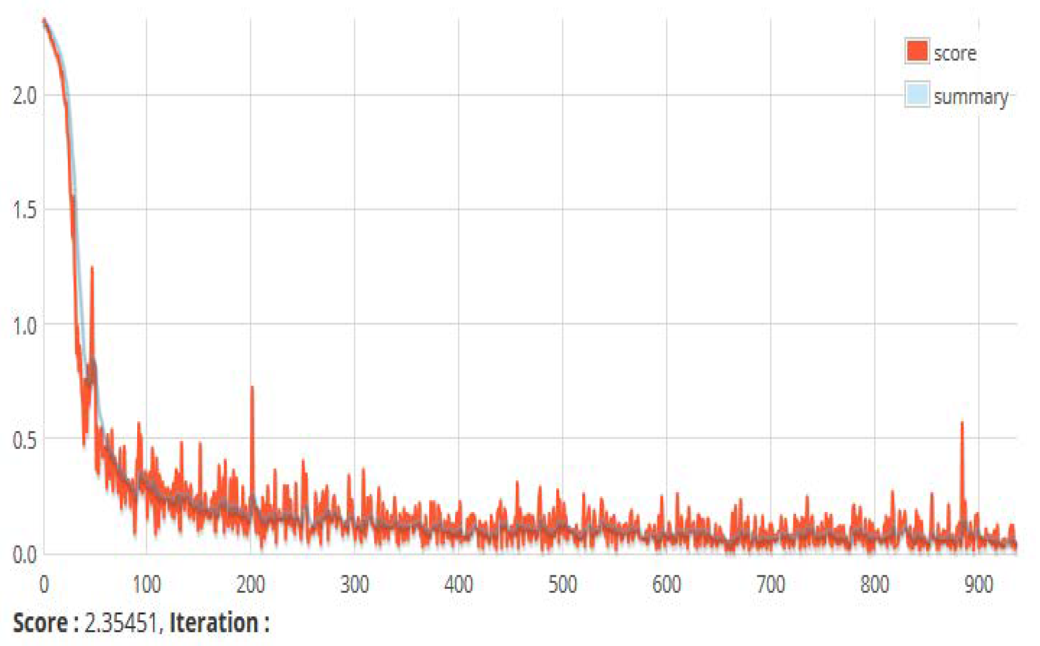
Figure 17.
A snapshot of the score versus iteration chart. This shows the value of the loss function of a currently running set of instances. The loss function depicts the mean square error between the actual and target output.
Figure 17.
A snapshot of the score versus iteration chart. This shows the value of the loss function of a currently running set of instances. The loss function depicts the mean square error between the actual and target output.
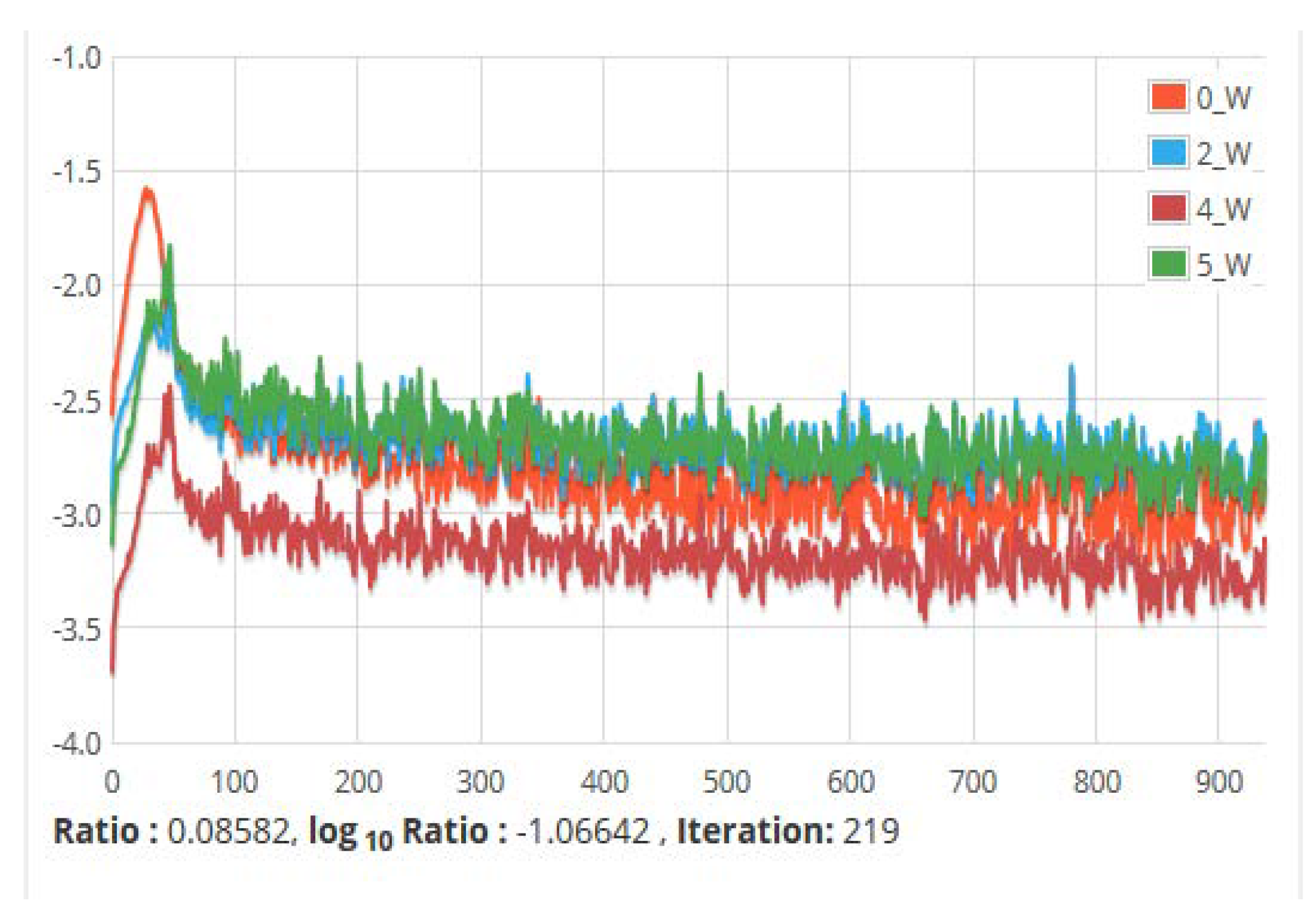
Figure 18.
The ratio of parameters to updates (by layer) for all network weights vs. Iteration. It shows the update of the parameters against the number of iterations taken during training.
Figure 18.
The ratio of parameters to updates (by layer) for all network weights vs. Iteration. It shows the update of the parameters against the number of iterations taken during training.
Figure 19.
Standard deviations of the activations, gradients and updates versus time. Updates refer to the update of the training parameters such as momentum and learning rate parameter.
Figure 19.
Standard deviations of the activations, gradients and updates versus time. Updates refer to the update of the training parameters such as momentum and learning rate parameter.
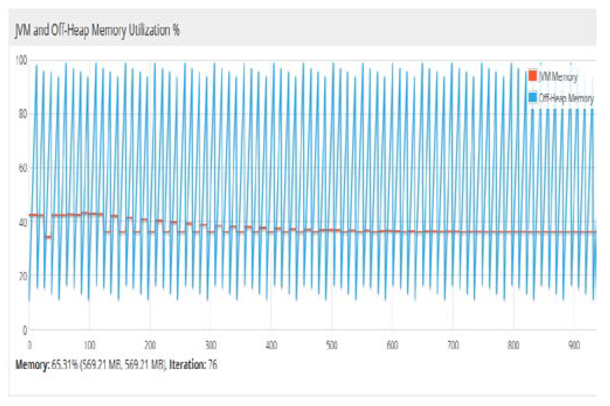
Figure 20.
Percentage of the main memory utilization for JVM and heap memory. In DL4j, off-heap memory is the portion of the main memory, which is not used by JVM. Therefore, the work of the garbage collector by JVM is limited. The off-heap memory management was carried out using the underlying native operating system.
Table 1.
Types of data used, their attributes, and their effect.
Table 1.
Types of data used, their attributes, and their effect.
| S.No | Type of Data | Attribute | Description and Effect | ![Computation 06 00062 i001]() |
| 1 | Clinical information of health data | SBP, DBP, HDL, LDL, triglycerides, cholesterol, micro-albumin, urine albumin-creatinine ratio, heart rate | These data can be captured by body sensors and have a high influence on hypertension attack. |
| 2 | Personal information | Height, weight, age, gender, the presence of disease in family history, smoking habits | Body mass index can be calculated, the presence of obesity is detected, the attack is also dependent on positive pedigree family history |
| 3 | Behavioral data | Stress level, type of stress, anxiety level, level of discomfort | Presence of stress may increase the risk of hypertension attack |
| 4 | Surrounding Data | Temperature, humidity, air quality | If temperature and humidity component have more than normal, the chances of attack will be more |
| 5 | GPS data | Location, time | The blood pressure reading will be more in high altitude regions and cold regions. | |
Table 2.
Categorization of stages of hypertension.
Table 2.
Categorization of stages of hypertension.
| Stage of Hypertension | SDP Reading | DBP Reading |
|---|
| Normal | Less than 120 | Less than 80 |
| Pre-hypertension | 120 ≤ SDP ≤ 139 | 80 ≤ DBP ≤ 89 |
| Hypertension Stage-1 | 140 ≤ SDP ≤ 159 | 90 ≤ DBP ≤ 99 |
| Hypertension Stage-2 | SDP ≥ 160 | DBP ≥ 100 |
| Hypertensive Crisis | SDP ≥ 180 | DBP ≥ 110 |
Table 3.
Datasets used, their attributes, and the source of data.
Table 3.
Datasets used, their attributes, and the source of data.
| Case Study Description | Data Attributes Used | Source of Data |
|---|
| Stress classification | EDA, HR, SpO2,temperature, 3-dimensional accelerometer data | www.utdallas.edu/~nourani/Bioinformatics/Biosensor_Data |
| Type-2 diabetes detection | PGC, DBP, 2-h serum insulin (mu U/mL) 4), body mass index (BMI), diabetes pedigree function, age in years | https://archive.ics.uci.edu/ml/datasets/Diabetes |
| Hypertension risk assessment | SBP, DBP, total cholesterol (TC), HDL, LDL, PGC and HR | http://archive.ics.uci.edu/ml, https://archive.ics.uci.edu/ml/datasets/Diabetes, https://archive.ics.uci.edu/ml/datasets/Chronic KidneyDisease, www.utdallas.edu/~nourani/Bioinformatics/Biosensor_Data |
Table 4.
Configuration of the deep neural network.
Table 4.
Configuration of the deep neural network.
| Dataset | No. of Inputs | No. of Outputs | No. of Hidden Layers | Learning Rate Parameter | Input and Hidden Layer Activation Function | Output Layer Activation Function |
|---|
| Diabetes | 7 | 2 | 2 | 0.1 | Tanh | SoftMax |
| Stress | 5 | 4 | 3 | 0.11 | ReLU | SoftMax |
| Hypertension | 8 | 2 | 2 | 0.13 | Tanh | SoftMax |
Table 5.
Performance matrix for diabetes mellitus prediction.
Table 5.
Performance matrix for diabetes mellitus prediction.
| Performance Matrix for Diabetes Dataset |
|---|
| Iteration = 1000, Learning Rate Parameter = 0.1 | Iteration = 5000, Learning Rate Parameter = 0.1 |
|---|
| Accuracy | Precision | Recall | F1 Score | Accuracy | Precision | Recall | F1 Score |
|---|
| 0.7398 | 0.7428 | 0.7173 | 0.6465 | 0.7812 | 0.7678 | 0.8173 | 0.6321 |
| 0.7872 | 0.7320 | 0.6989 | 0.6000 | 0.7974 | 0.7458 | 0.6889 | 0.6122 |
| 0.7770 | 0.7523 | 0.7496 | 0.6703 | 0.8387 | 0.8523 | 0.7496 | 0.6898 |
| 0.7361 | 0.7189 | 0.6900 | 0.5896 | 0.8411 | 0.7189 | 0.6990 | 0.5987 |
| 0.7955 | 0.7761 | 0.7774 | 0.7120 | 0.8199 | 0.8773 | 0.7874 | 0.7234 |
| 0.7658 | 0.7416 | 0.7323 | 0.6480 | 0.8452 | 0.8428 | 0.7323 | 0.6346 |
| 0.8578 | 0.8861 | 0.7865 | 0.6632 | 0.8623 | 0.8873 | 0.8165 | 0.6789 |
| 0.7807 | 0.7825 | 0.7413 | 0.6667 | 0.8383 | 0.7897 | 0.7413 | 0.6782 |
| 0.8387 | 0.7243 | 0.6916 | 0.6900 | 0.8655 | 0.7255 | 0.6916 | 0.6989 |
| 0.7955 | 0.7761 | 0.7774 | 0.7120 | 0.7989 | 0.7773 | 0.7888 | 0.7121 |
| 0.7658 | 0.7420 | 0.7156 | 0.6182 | 0.8231 | 0.8432 | 0.7234 | 0.6261 |
| 0.7918 | 0.7643 | 0.7553 | 0.6710 | 0.8490 | 0.7655 | 0.7678 | 0.6711 |
| 0.8123 | 0.8302 | 0.6767 | 0.6547 | 0.8767 | 0.8314 | 0.6897 | 0.6245 |
| 0.8545 | 0.8489 | 0.6547 | 0.6400 | 0.8786 | 0.8501 | 0.6676 | 0.6534 |
| 0.7998 | 0.6756 | 0.6511 | 0.6100 | 0.7889 | 0.6768 | 0.6456 | 0.6298 |
| 0.7876 | 0.8156 | 0.6978 | 0.6001 | 0.8456 | 0.8168 | 0.7123 | 0.6122 |
| 0.8356 | 0.7889 | 0.6900 | 0.6032 | 0.8891 | 0.8100 | 0.7898 | 0.6977 |
| 0.8321 | 0.8213 | 0.6763 | 0.5432 | 0.8134 | 0.8225 | 0.6932 | 0.5771 |
| 0.8563 | 0.8600 | 0.6789 | 0.6523 | 0.8651 | 0.8612 | 0.6897 | 0.678 |
| 0.8490 | 0.8345 | 0.6751 | 0.6800 | 0.8989 | 0.7578 | 0.6451 | 0.6898 |
| Average value over 20 iterations |
| 0.802945 | 0.7807 | 0.71169 | 0.64355 | 0.840845 | 0.8010 | 0.726845 | 0.65593 |
Table 6.
Performance matrix for the stress classification model.
Table 6.
Performance matrix for the stress classification model.
| Performance Matrix for Stress Dataset |
|---|
| Iteration = 1000, Learning Rate Parameter = 0.1 | Iteration = 5000, Learning Rate Parameter = 0.1 |
|---|
| Accuracy | Precision | Recall | F1 Score | Accuracy | Precision | Recall | F1 Score |
|---|
| 0.871 | 0.8539 | 0.8173 | 0.7677 | 0.8822 | 0.8551 | 0.8182 | 0.7668 |
| 0.9184 | 0.8421 | 0.81 | 0.7112 | 0.9297 | 0.8434 | 0.8108 | 0.712 |
| 0.9082 | 0.8534 | 0.8707 | 0.7715 | 0.9194 | 0.8548 | 0.8714 | 0.7804 |
| 0.8673 | 0.83 | 0.78 | 0.6808 | 0.8785 | 0.8312 | 0.7889 | 0.6896 |
| 0.8267 | 0.8872 | 0.8685 | 0.7932 | 0.8379 | 0.8881 | 0.86938 | 0.8019 |
| 0.897 | 0.8527 | 0.8323 | 0.7492 | 0.9082 | 0.8538 | 0.8332 | 0.7559 |
| 0.989 | 0.8873 | 0.8865 | 0.7844 | 1.0002 | 0.8885 | 0.8866 | 0.7845 |
| 0.9119 | 0.8805 | 0.8413 | 0.7879 | 0.9233 | 0.8819 | 0.8419 | 0.7886 |
| 0.9587 | 0.8223 | 0.7916 | 0.8112 | 0.9699 | 0.8313 | 0.7925 | 0.8200 |
| 0.7967 | 0.8872 | 0.8774 | 0.8332 | 0.8079 | 0.8883 | 0.8782 | 0.8243 |
| 0.877 | 0.8531 | 0.8156 | 0.7394 | 0.8882 | 0.8547 | 0.8244 | 0.7472 |
| 0.923 | 0.8754 | 0.8553 | 0.7922 | 0.9342 | 0.8767 | 0.864 | 0.7923 |
| 0.9135 | 0.9413 | 0.7767 | 0.7759 | 0.9247 | 0.9493 | 0.7776 | 0.7761 |
| 0.8557 | 0.91 | 0.7547 | 0.7612 | 0.8669 | 0.9115 | 0.7625 | 0.7609 |
| 0.931 | 0.7867 | 0.7511 | 0.7312 | 0.9422 | 0.7965 | 0.7600 | 0.7316 |
| 0.9188 | 0.9267 | 0.7978 | 0.7213 | 0.932 | 0.9284 | 0.7983 | 0.7214 |
| 0.9356 | 0.9 | 0.79 | 0.7244 | 0.9368 | 0.9011 | 0.7988 | 0.7255 |
| 0.8933 | 0.9324 | 0.7763 | 0.6644 | 0.9045 | 0.9336 | 0.784 | 0.66441 |
| 0.9683 | 0.9101 | 0.7789 | 0.7735 | 0.9783 | 0.9113 | 0.7798 | 0.77437 |
| 0.9502 | 0.9456 | 0.7751 | 0.8012 | 0.9617 | 0.9468 | 0.7760 | 0.8013 |
| Average value over 20 iterations |
| 0.905565 | 0.8918 | 0.812355 | 0.75875 | 0.916335 | 0.881315 | 0.815824 | 0.760954 |
Table 7.
Performance matrix of the hypertension risk assessment model.
Table 7.
Performance matrix of the hypertension risk assessment model.
| Performance Matrix for Hypertension Dataset |
|---|
| Iteration = 1000, Learning Rate Parameter = 0.1 | Iteration = 5000, Learning Rate Parameter = 0.1 |
|---|
| Accuracy | Precision | Recall | F1 Score | Accuracy | Precision | Recall | F1 Score |
|---|
| 0.8398 | 0.8339 | 0.8173 | 0.7677 | 0.8510 | 0.9151 | 0.8182 | 0.7668 |
| 0.9184 | 0.8321 | 0.8100 | 0.7112 | 0.9297 | 0.9134 | 0.8108 | 0.7120 |
| 0.8782 | 0.8334 | 0.8707 | 0.7715 | 0.8894 | 0.9148 | 0.8714 | 0.7804 |
| 0.8673 | 0.7800 | 0.7801 | 0.6808 | 0.8785 | 0.8612 | 0.7889 | 0.6896 |
| 0.8267 | 0.7872 | 0.8685 | 0.7932 | 0.8379 | 0.8681 | 0.86938 | 0.8019 |
| 0.8970 | 0.7627 | 0.8323 | 0.7492 | 0.9082 | 0.8438 | 0.8332 | 0.7559 |
| 0.9890 | 0.8873 | 0.8865 | 0.7844 | 1.0002 | 0.9685 | 0.8866 | 0.7845 |
| 0.8819 | 0.8805 | 0.8413 | 0.7879 | 0.8933 | 0.9619 | 0.8419 | 0.7886 |
| 0.8507 | 0.8223 | 0.7916 | 0.8112 | 0.8619 | 0.9113 | 0.7925 | 0.8200 |
| 0.8267 | 0.8872 | 0.8774 | 0.8332 | 0.8379 | 0.9683 | 0.8782 | 0.8243 |
| 0.8870 | 0.8531 | 0.8156 | 0.7394 | 0.8982 | 0.9347 | 0.8244 | 0.7472 |
| 0.9030 | 0.8754 | 0.8553 | 0.7922 | 0.9142 | 0.9567 | 0.864 | 0.7923 |
| 0.8243 | 0.9413 | 0.7767 | 0.7759 | 0.8355 | 0.9700 | 0.7776 | 0.7761 |
| 0.8557 | 0.91 | 0.7547 | 0.7612 | 0.8669 | 0.9915 | 0.7625 | 0.7609 |
| 0.8310 | 0.7867 | 0.7511 | 0.7312 | 0.8422 | 0.8765 | 0.7600 | 0.7316 |
| 0.8888 | 0.8157 | 0.7978 | 0.7213 | 0.902 | 0.8974 | 0.7983 | 0.7214 |
| 0.8456 | 0.7891 | 0.7900 | 0.7244 | 0.8468 | 0.8702 | 0.7988 | 0.7255 |
| 0.8933 | 0.8217 | 0.7763 | 0.6644 | 0.9045 | 0.9029 | 0.7840 | 0.66441 |
| 0.8675 | 0.8651 | 0.7789 | 0.7735 | 0.8775 | 0.9463 | 0.7798 | 0.77437 |
| 0.8502 | 0.8556 | 0.7751 | 0.8012 | 0.8617 | 0.9287 | 0.7760 | 0.8013 |
| Average value over 20 iterations |
| 0.871105 | 0.841015 | 0.812355 | 0.75875 | 0.881875 | 0.920056 | 0.815824 | 0.760954 |
Table 8.
Comparative analysis of stress classification.
Table 8.
Comparative analysis of stress classification.
| Author | Tools Used for Application Development | Purpose | Accuracy of Prediction Model | Data Used | Whether Used in Fog Environment |
|---|
| M.M. Sami et al. (2014) [67] | Support vector machine | Stress classification model | 83.33% | EEG Signals | No |
| Q. Xu et al.(2015) [68] | K-Means clustering algorithm | To provide personalized recommended products for stress management | 85.2% | EEG, ECG, EMG, GSR signals | No |
| S. H. Song et al. (2017) [69] | Deep belief network | To design stress monitoring system | 66% | KNHANES VI | No |
| Deep-Fog | Deep neural network | To obtain the stress level of patients to assist doctors | 91.63% | EDA, HR, SpO2, Temperature | Yes |
Table 9.
Comparative analysis of diabetes prediction.
Table 9.
Comparative analysis of diabetes prediction.
| Method | Accuracy (%) | Use Cloud for Storage | Used in Fog Environment | Author |
|---|
| Hybrid model | 84.5% | No | No | HumarKehramanili (2008) [70] |
| Multilayer perceptron | 81.90% | No | No | Aliza Ahmed et al. (2011) [71,72] |
| Decision tree | 89.30% | No | No | Aliza Ahmed et al. (2011) [71] |
| Extreme learning machine | 75.72% | No | No | R. Priyadarshini et al. (2014) [73] |
| Decision tree | 84% | No | No | K.M.Orabi et al. (20216) [74] |
| Improved K-means andlogistic regression | 95.42% | No | No | Han Wu et al. (2017) [60] |
| Proposed approach | 84.11% | Yes | Yes | |
Table 10.
Comparative analysis of Hypertension risk detection.
Table 10.
Comparative analysis of Hypertension risk detection.
| Author | Application Domain | Purpose | Use of CS | Use in FE | Use of PM |
|---|
| Fernandez et al. (2017) [75] | A web-based hypertension monitoring system | To identify weakness in the clinical process of hypertension detection, to improvise the existing system | No | No | No |
| Zhou et al. (2018) [76] | Cloud and mobile internet-based hypertension management system | Provide services to the patient to let them know their cardiac status | Yes | No | No |
| S.Sood and Isha Mahajan (2018) [77] | IoT-fog based system | Real time monitoring and decision making | Yes | Yes | Back propagation neural network with precision 92.10% |
| Proposed Work-Deep Fog | Deep learning-based Fog system | Real time Assessment of hypertension in patients and sending the data to cloud | Yes | Yes | Deep neural network with precision 92.01% |
Table 11.
Software information.
Table 11.
Software information.
| Host Name | OS | OS Architecture | JVM Name | JVM Version | ND4J Backend | ND4J Type |
|---|
| 3LAB24-PC | Windows 7 | Amd64 | Java Hotspot (TM)64-bit Server VM | 1.8.0_141 | CPU | Float |
Table 12.
Hardware information.
Table 12.
Hardware information.
| JVM Current Memory | JVM Max Memory | Off-Heap Current Memory | Off-Heap Max Memory | JVM Available Processors | #Compute Devices |
|---|
| 315.50 MB | 871.50 MB | 451.22 MB | 871.50 MB | 4 | 0 |


