1. Introduction
An urban environment is an assembly of buildings, parks, commercial and industrial areas, public buildings, and infrastructure such as roads, railways, and airports. The human activity inside the city could cause serious accidents with hazardous release incidents. The air flow distribution and the turbulent diffusion phenomena at the complex environment of a city could result in an unpredictable evolution of an urban accident. This complexity could constitute an impediment to the proper intervention and the accident’s management. Therefore, it is important to understand the urban structure and its form, in order to prevent serious toxic release incidences. The main units of an urban environment are the urban building blocks. These define the flow distribution inside the city’s environment.
Some field experiments have investigated the pollutant dispersion in a city [
1,
2,
3]. Yet, field experiments for pollutant dispersion in an urban environment are very difficult and costly. This is the main reason why Computational Fluid Dynamics (CFD) could be a simpler approach for these kinds of studies. Different CFD techniques could be applied to study an urban dispersion problem, such as the Reynolds Average Navier Stokes (RANS) models [
4,
5,
6], the Large eddy Simulation (LES) models, the Implicit-eddy Large Simulation (ILES) models [
7,
8] and the Direct Numerical (DNS) models. The air flow within the urban atmospheric boundary layer was also experimentally studied with wind tunnel experiments [
9].
In order to define the complex phenomena of an urban geometry, simplified cases for the urban building blocks were studied. The urban building blocks areas can be simplified into arrays with rectangular buildings. Urban building blocks are characterized by buildings’ height and the space between them [
10,
11]. Different studies exist for the study of the flow into elementary urban units such as the street canyons [
12,
13,
14,
15,
16,
17,
18,
19,
20,
21]; the street intersections [
22,
23,
24]; the influence of tall buildings in the urban environment [
25,
26] and in open spaces [
27]. Moreover, the flow and pollution dispersion around staggered and aligned groups of cube arrays have been examined [
28].
A pool fire accident may occur in a road between urban building blocks. Several studies in an open space pool fire accident exist [
29,
30,
31,
32,
33,
34,
35], as well as for a pollutant dispersion in a street canyon [
17,
18,
36,
37]. However, only a few of them focus on the study of a fire accident inside a street canyon [
21,
38,
39,
40,
41,
42]. The pollutant dispersion into an array of cubes has been studied experimentally and computationally [
10,
43,
44]; however, there is a lack of documentation for a fire incident inside an array of cubes.
The current study presents appropriate computational techniques for the prediction of a toxic release in an urban environment after a fire accident. It also presents a qualitative and quantitative analysis for different urban geometries to predict the immediately dangerous to life or health (IDLH) smoke zones. A Large eddy Simulation technique is applied and defined in
Section 2. The simulation’s results are discussed in
Section 3. Finally, the conclusions are in
Section 4.
2. Computational Characteristics
2.1. Flow Field Definition
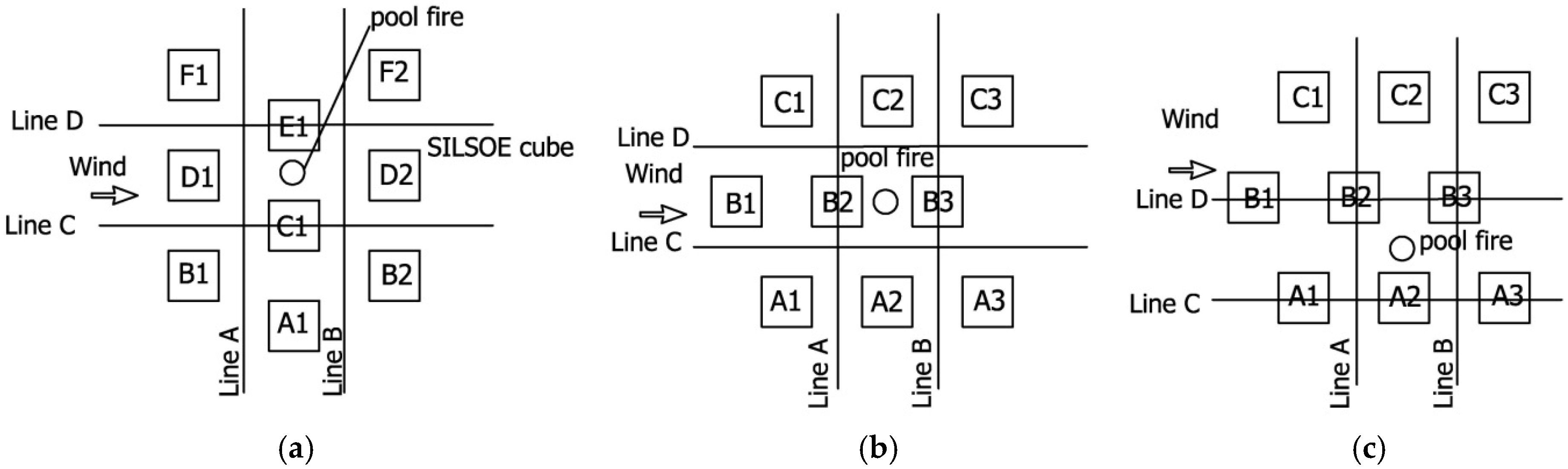
A simplified urban domain model of nine cubes in different rectangular staggered arrays was studied as is shown in
Figure 1. This cube’s arrangement is similar to the Silsoe cube arrays research site [
45,
46]. In
Figure 1a, the D2 cube is the Silsoe cubical building. The surface pressure of the Silsoe cube was experimentally measured with pressure taps; thus, the present numerical model was successively validated against these measurements as discussed in the next Section. Three different cubes arrangements and the smoke fire dispersion from different diesel pool fire locations were considered as shown in
Figure 1. Each column array was marked with a unique letter. All cubes were of an
H = 6 m height and they were shifted in lines and columns of 6 m distance. For Case 1, the pool fire was placed between the D1 and D2 cubes that were in a distance
3H and C1 and E1 cubes that were in the distance
H. For Case 2, the pool fire was placed between B2 and B3 cubes that were in distance
H and A2 and C2 cubes that were in distance
3H. Finally, for Case 3, the pool fire was placed between A and B columns. The wind flow direction in each Case is also shown in
Figure 1. The smoke concentration level was studied along A, B, C, and D lines. All the lines were placed at an H distance from the center of the diesel pool fire accident.
The computational domain was extended at X = 20
H, Y = 20
H, and Z = 8
H in the streamwise, the perpendicular, and the height direction. For each case, the diesel pool fire was set at the center of the domain as shown in
Figure 1 at X = Y = Z = 0.
2.2. Fundamental Equations
The Fire Dynamics Simulation (FDS) is a low-speed code (the Mach number is less than 0.3) that numerically solves the Navier-Stokes equations. It was applied to thermally driven flow. The FDS model was validated against a wide variety of full scale experiments. The FDS model is a low Mach, Large eddy Simulation code. A low pass-filter was applied for the derivation of the mass, momentum, and energy equations. The Smagorinsky form of the LES models was applied to define the turbulence characteristics [
47].
The LES approach develops the filtered mean values of mass, momentum, and energy and takes into account the effect of the subgrid model. A mass-weighted Favre filter was applied such as . The filtered field, denoted with a bar and with the “” symbol, was denoted the mass-weighted mean property.
The Favre-filtered equations are:
where,
is the density,
g is the gravity acceleration,
u is the velocity, p is the pressure,
t is the time, and
is the stress tensor.
The filter advection term is , where is the subgrid scale stress (SGS). The SGS is decomposed and the Newton’s law of viscosity is applied.
The filter Navies Stokes equation is reformed as [
47]:
where
is the total deviatoric stress and is expressed as
, μ is the dynamic viscosity of the fluid,
is the strain tensor, and
is the Kronecker delta.
The turbulent viscosity
is modeled with the Smagorinsky analysis as:
is the Smagorinsky coefficient, Δ is the filter lengthscale.
The energy conservation equation is written as:
where,
is the sensible enthalpy,
is the heat release per unit volume from the chemical reaction,
are the radiative and conductive heat fluxes,
is the Prandtl number, and
is the turbulent Prandtl number with value 0.5.
The transport equation for species is written as:
where,
is the diffusivity of species
i,
is the mass fraction of species
i, and
is turbulent Schmidt number with value 0.8.
2.3. Numerical Details and Validation
An explicit predictor-corrector finite difference scheme was applied. This scheme was second order accurate in time and space. In each time step, the Poisson equation for modified pressure was solved by a direct FFT-based solver. An explicit second-order Runge-Kutta scheme was applied for the flow variables which were updated in time.
The convective terms were upwind-biased differences in the predictor step and downwind biased differences in the corrector step. The material and thermal diffusion terms were central differences, with no upwind or downwind bias. The same difference was used during the predictor and corrector steps. FDS uses a structured staggered grid with the immersed boundary method (IBM) for the treatment of the flow obstruction [
48].
The computational mesh is important for the accuracy of the numerical model. The characteristic grid spacing is defined from the expression [
47]:
where,
is the ambient air temperature,
is the specific heat,
is the air density,
g is the gravitational acceleration, and
Q is the heat rate release. A uniform grid size was applied at the computational domain with a value equal to
. The numbers of cells were 5,200,000, and the duration of the simulation lasts for 250 s.
During the calculation, the time step was adjusted so that the Courant–Friedrichs–Lewy (CFL) condition should be lower than 1 (CFL < 1). The averaging of fluid flow and transport quantities were recorded between 100 s, where the fire dispersion starts, and 250 s. The initial transient at 100 s was adequate for the flow field to become stationary. The concentration averaged at 250 s when the smoke plume was fully developed.
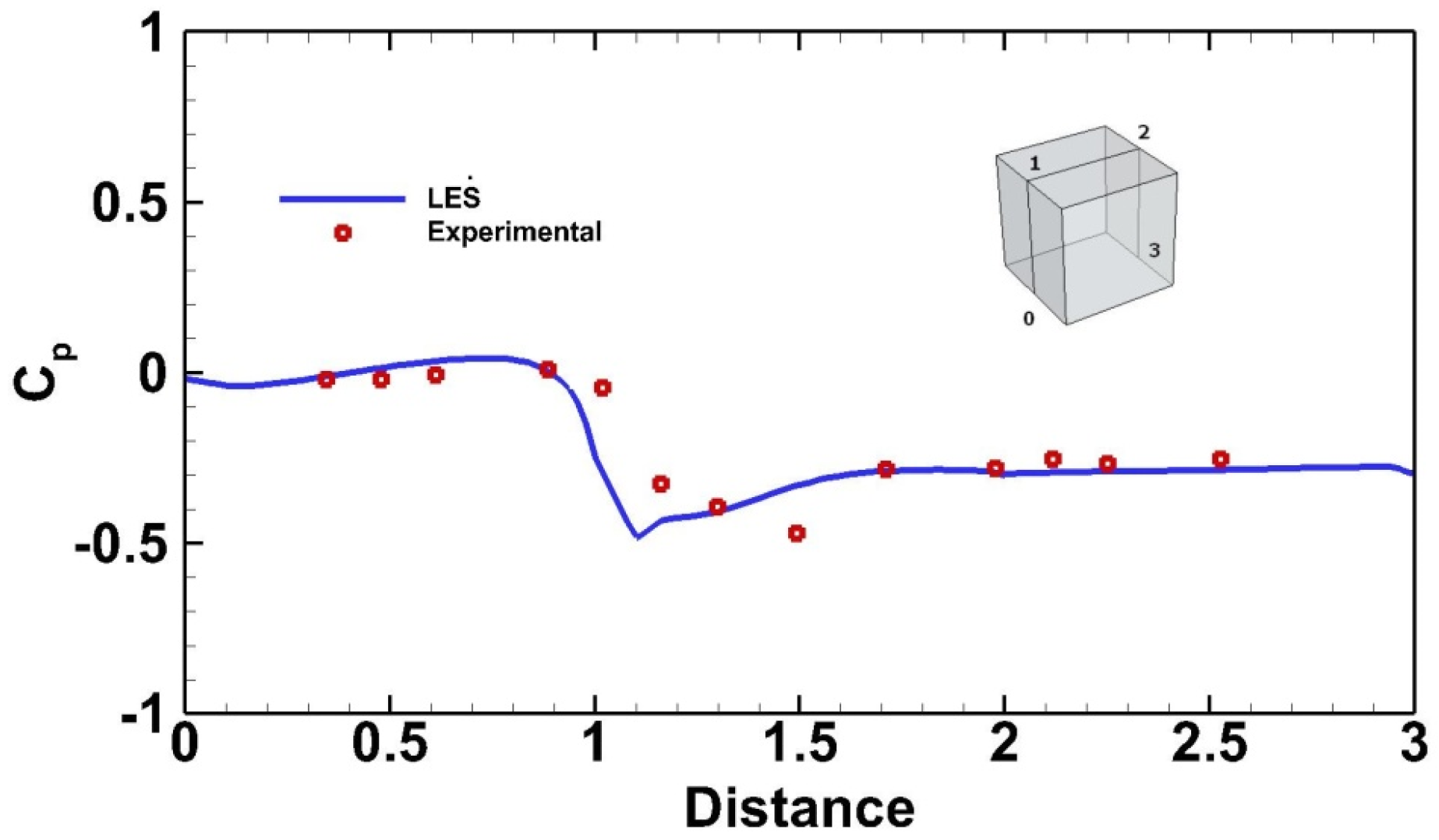
Results from the present simulations were compared successively against experimental data [
45,
46] for the pressure coefficient,
, defined by:
where,
, is the local static pressure,
, is free-stream static pressure, and
is the free stream velocity. As shown in
Figure 2, the present numerical results were fairly good as compared against the experimental results of the Silsoe cube.
2.4. Boundary Conditions
The Silsoe research site experimental data were applied for the inlet velocity condition [
49]. The velocity at the inlet boundary condition was applied as:
where
κ = 0.4 is the von Karman’s constant,
is the reference height,
= 0.01 m is the ground roughness height [
50], and the undisturbed approach of the flow velocity at the cube’s height is
Uref = 10.08 m/s.
The lateral boundary conditions were set as periodic. An open boundary where the fluid is allowed exit from the computational domain was applied at the outflow condition. At the outflow boundary, the standard zero gradient condition was applied. The floor of the domain and the cube’s wall were modeled with a log-law velocity profile.
2.5. Diesel Pool Fire
A fire is a reaction of a hydrocarbon fuel with oxygen that produces carbon dioxide and water vapor. Most of the time, air is inefficient, and this has as a result the production of multiple combustion products. In order to limit the computational time, a simplified approach to the chemistry was applied involving six gas species (Fuel, and soot particles. The air, the fuel, and the fire products are referred to as ‘lumped species’. Fuel and products species were explicitly computed. The lumped species approach was the accordance with the mass transport equations.
The diesel pool fire incident had a
D = 3 m diameter. The incident had the same characteristics of the Chatris, Quintela [
31] experimental study with different geometry and wind flow conditions. The fuel mass loss rate
and the total heat release rate
(HRR) were defined by the following equations [
51]:
where,
is the infinite-diameter pool mass-loss rate,
is the heat of combustion
is the surface area of the pool,
β is the “mean beam length corrector”, and
k is the absorption extinction coefficient of the flame.
According to the experimental results, the mass burning rate for a diesel pool fire with a 3 m diameter is about 0.045 and the total heat release rate (HRR) is 13.5 MWatt.
Another important parameter in order to define the smoke products is the smoke yield. The smoke yield is defined as the amount of burned fuel (kg smoke/kg fuel). Walton et al. [
52] assumed that the smoke yield from a diesel firevaries between 15% and 20%; Argyropoulos [
33] proposed an average 17.5% for the smoke yield. In our study, the smoke yield is defined as 17.5%.
Assael and Kakosimos [
53] defined the risk zones where the toxic concentration could place the human’s health in danger. A risk zone is a circular area which has as a center at the point of the source emission, and is extended to the limit where safety is ensured. Risk zones cover incidents of heat flux and toxic substance in case of fires. Different zones are defined:
- (a)
Zone I—Very Serious Consequences, Lethal Concentration 50% (LC50 region). The possibility of death population in this zone is 50% due to inhalation of a toxic substance.
- (b)
Zone ΙΙ—Serious Consequences, Lethal Concentration 1% (LC1 region). The possibility of death population in this zone is 1% due to inhalation of a toxic substance.
- (c)
Zone III—Moderate Consequences,Immediately Dangerous to Life and Health (IDLH region) . Zone III could lead to reversible injuries following the inhalation of a toxic substance. Outside the Zone III is the safe area.
The values of the safety limits of the fire smoke pollutants are defined from the National Institute for Occupational Safety and Health (NIOSH) as LC1 = 25,000 (mg/m3) and IDLH = 2500 (mg/m3).
3. Results and Discussion
3.1. Flow Field Results
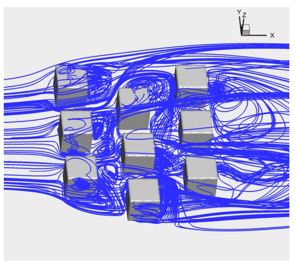
The FDS code performs large eddy Simulations analysis for a diesel pool fire accident inside an array of cubes. The mean flow in the staggered cubes array is very complicated as it is characterized by different vortices as shown in the streamlines of
Figure 3. It is detached on the roof top of the buildings and forms vortices simultaneously with the side vortices that are also formed at the buildings. These vortices enter inside the street intersections and influence the flow characteristics inside the cubes’ rows and columns. Important helicoid vortices are formed behind the buildings of the first column which are responsible for the fire’s products dispersion. This phenomenon is decreasing in the second column of the array, and finally, wake vortices are formed behind the last column of the cubes.
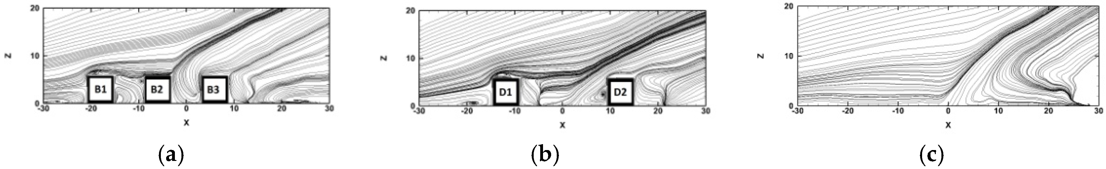
In Case 1, the cube lines were staggered perpendicular of the wind direction which means that the wind did not flow symmetrically. As shown in
Figure 4a for the streamlines at the plane
Z = 1 m, the asymmetry had an important effect to the flow distribution. Two recirculations behind the D1 cube and a smaller one at the lateral face appeared. The streamlines diverged between the C1 and E1 cubes, at the pool fire incidence location. A smaller lateral recirculation appeared at the lateral face of the C1 cube. In contrast, Case 2 led to a more symmetrical flow. As shown in
Figure 4b, similar mirror recirculations appeared at the fire symmetry axis,
Y = 0, while the streamlines at the fire position reversed towards the Cube B2. Finally, the streamlines of Case 3 are presented in
Figure 4c. It was found that the pool fire location was not affected by the cube’s recirculation zone. The buoyancy forces were so strong that an important asymmetry was found and a major horizontal recirculation zone formed inside the street canyon.
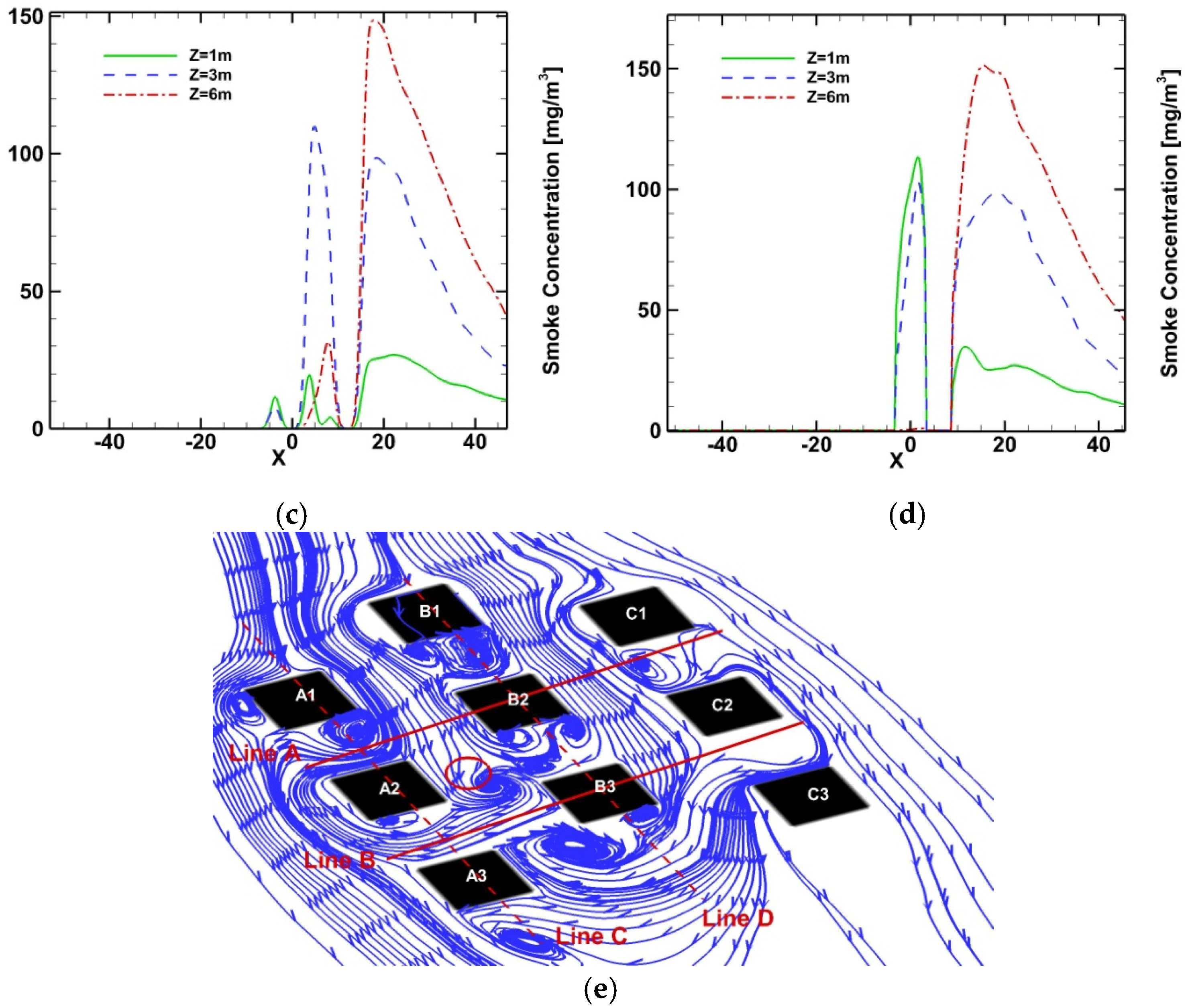
Figure 5a–c present the time-average streamlines for the fire symmetry plane at
Y = 0 m for the Cases 1, 2 and 3, respectively. From this figure, it is shown that the buoyancy-driven forces due to the fire are relatively stronger in the vertical direction than the wind inertia forces. This phenomenon leads the smoke dispersion patterns outside the cube’s array.
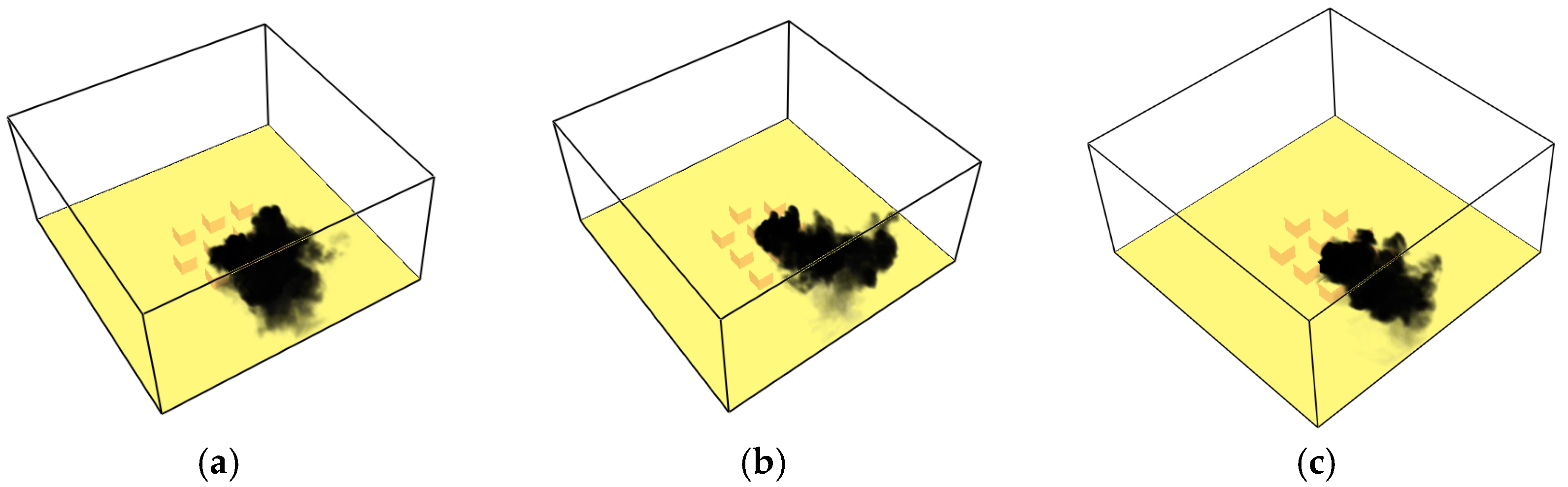
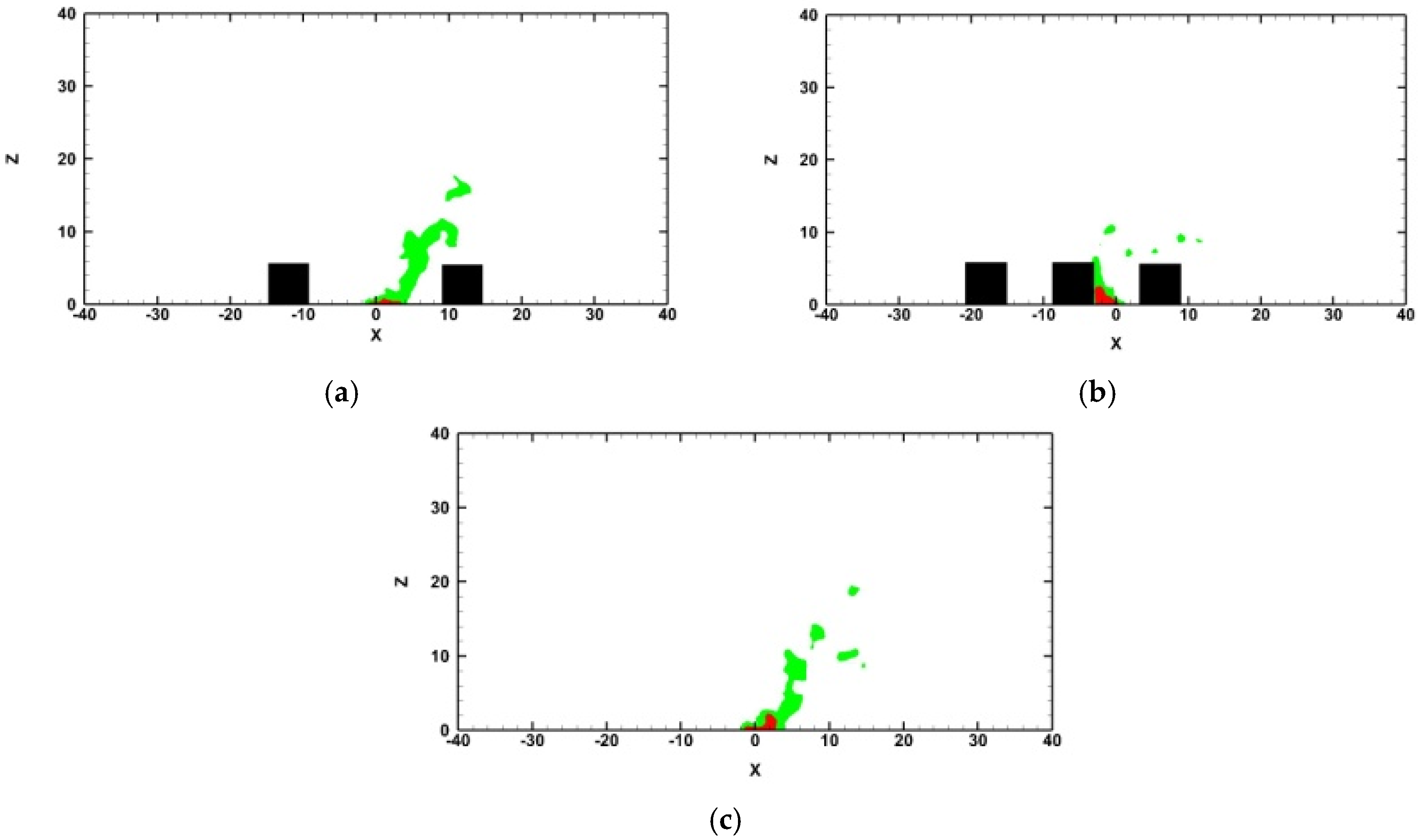
Figure 6 shows the smoke dispersion snapshots of the diesel pool fire after 200 s of the incidence for the three studied cases. The general observation is that the smoke plume was driven by the buoyancy forces and the wind flow, and reached at the top of the cube’s arrays. Due to the importance of the buoyancy forces, the smoke was moved outside the arrays, and only a small part of it recirculated between the cubes.
The identification of vortices and coherent structures could be made with the iso-surfaces of the Q-criterion. The Q-criterion is defined as:
where,
is a constant for the impressions,
is the strain rate, and
is the vorticity rate tensors.
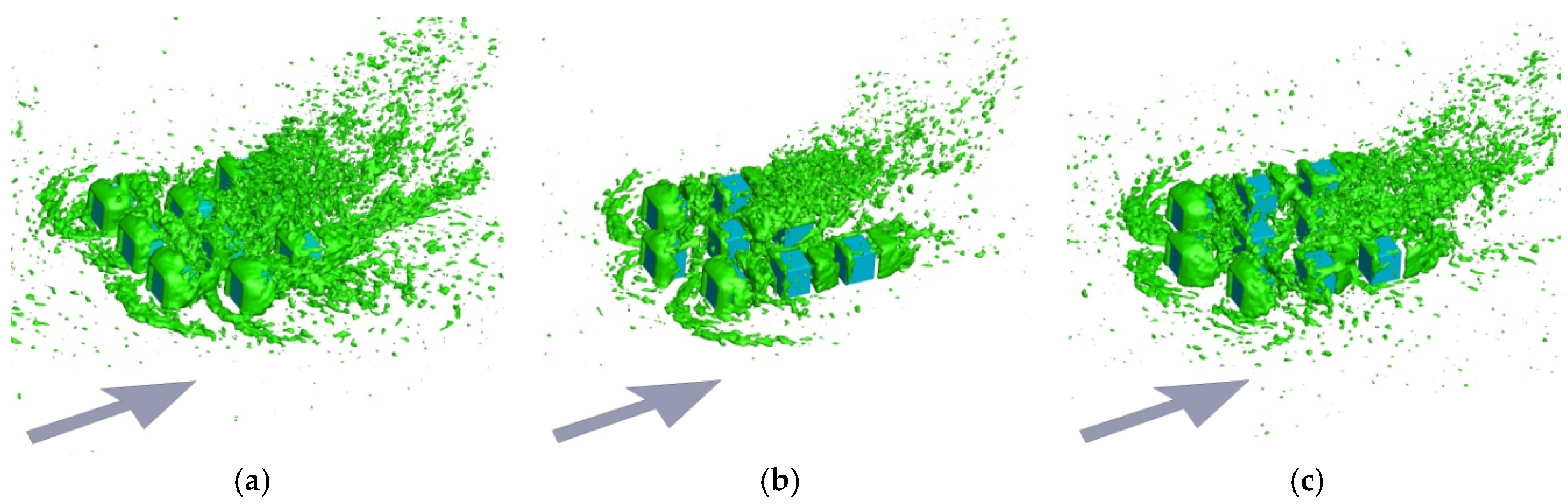
In
Figure 7 the Q = 0.1 level was selected to better visualize the turbulent structures for the three different cases. It can be seen that the horseshoe vortex formed on the leeward face of all the cubes that are in the direction of the induced wind. Hairpin vortices are formed for all array cubes of Case 1, while for Case 2 and 3, hairpin vortices formed only for the first line of the array cubes that faced the incoming wind. The pool fire source for Case 1 and 2 was located in the wake zone of D1 and B2 cubes, respectively. The flow inside these wake zones formed a strong mixing and turbulence generation region. As shown in
Figure 7, a fire accident produced important coherent structures that exceeded the cubes array height.
3.2. Smoke Concentration
Figure 8,
Figure 9 and
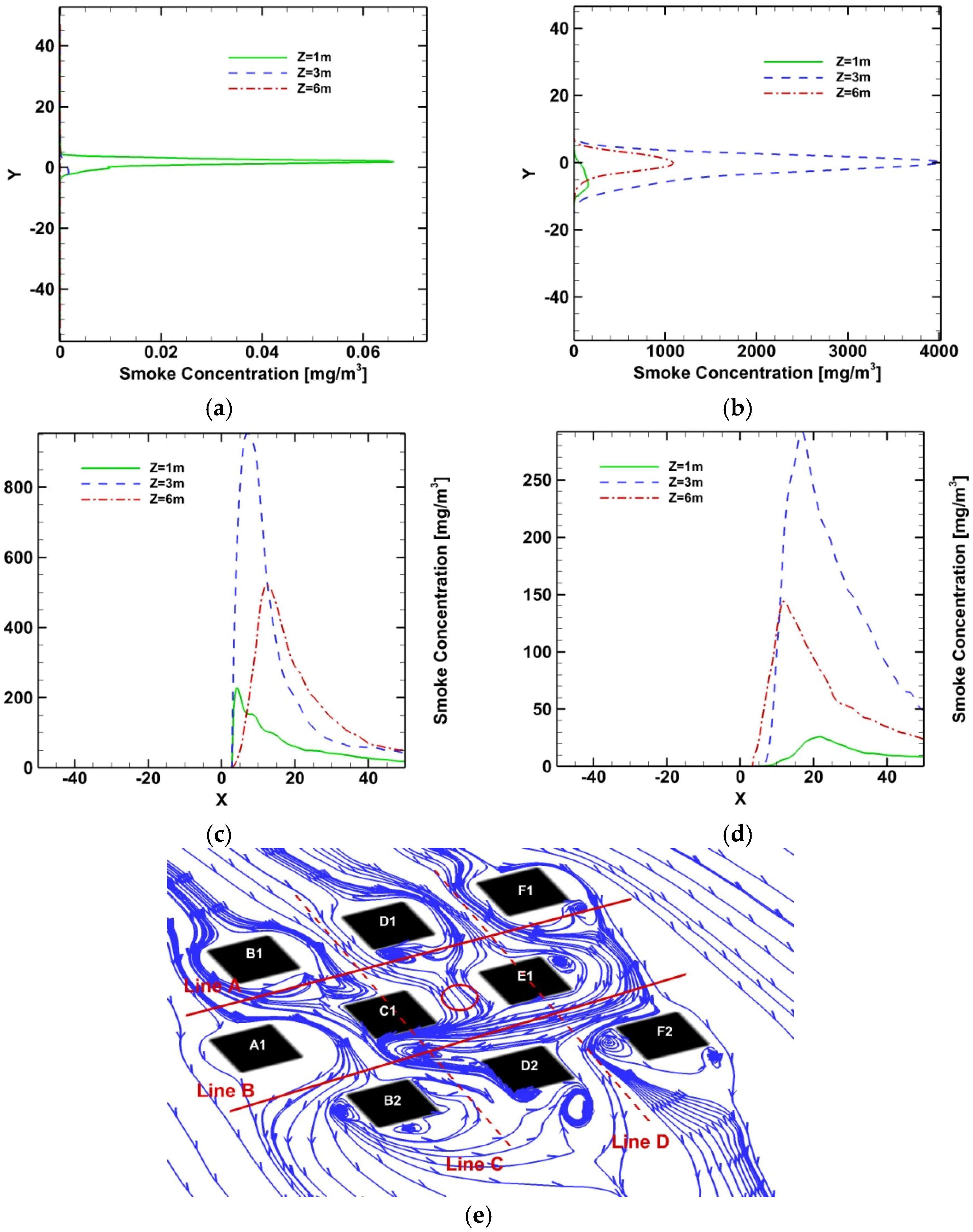
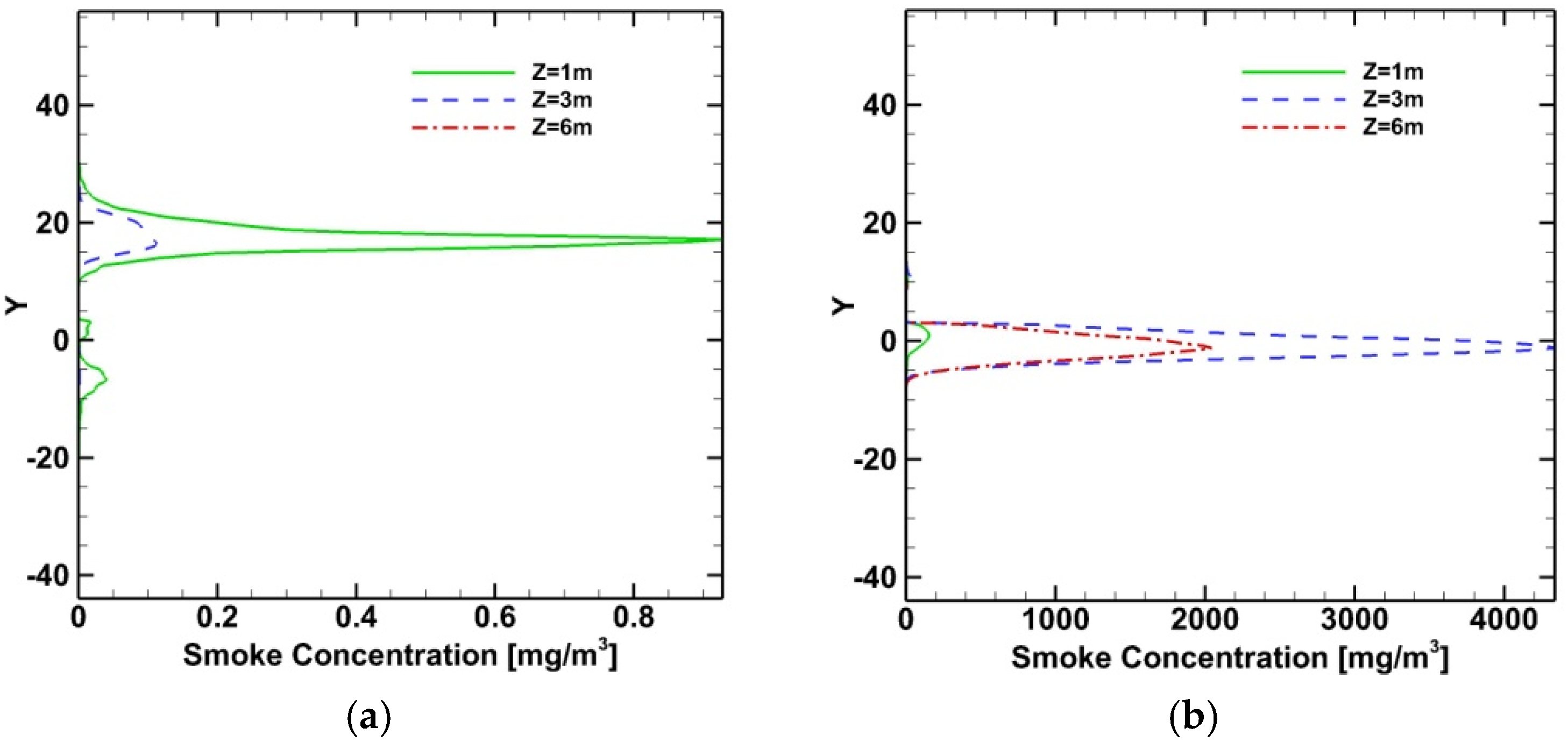
Figure 10 show the average smoke concentration along A, B, C and D lines for Case 1, Case 2 and Case 3, respectively. As shown in
Figure 8a, the smoke concentration leeward the fire position (A line) is negligible.
As shown from the streamlines on
Figure 8e, the smoke was channeled along line B. Additionally, an important recirculation zone was created leeward of the C1 cube, which trapped the smoke. In this region, the smoke concentration reached its highest limits. Additionally, the smoke concentration had higher values at the
Z = 3 m level (
Figure 8b). Along line C (
Figure 8c) the smoke concentration was more important than this of line D (
Figure 8d).
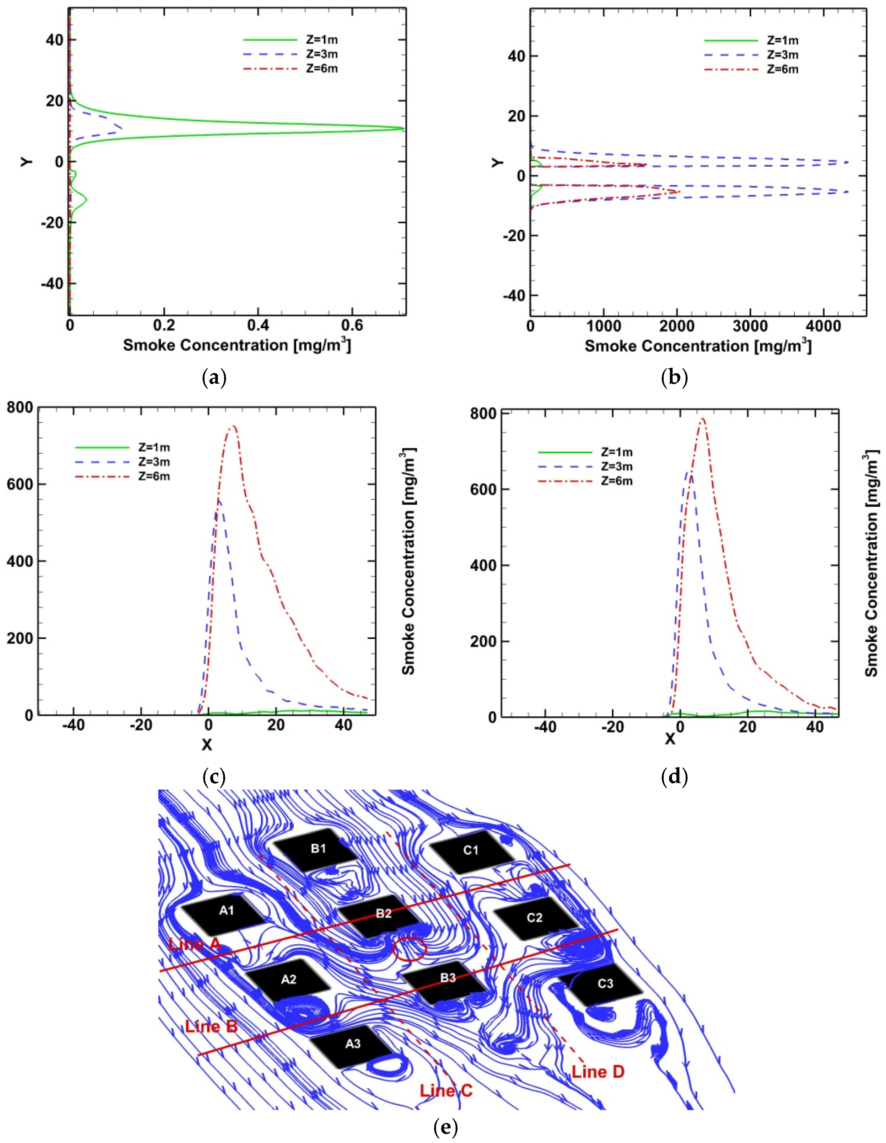
Figure 9a shows that the smoke concentration at the windward line A of the fire position was minimum; however, it presented slightly higher values than in Case 1.
Figure 9b shows that the maximum values of smoke concentration were presented at the lateral sides of the B3 cube. As shown in
Figure 9c,d, the smoke concentration distribution was quite similar for both C and D lines. This is due to the symmetry of the flow and the pool’s fire position.
Finally, in
Figure 10a, the smoke concentration at the leeward line A of the fire position was also minimum. Along line B (
Figure 10b), the smoke concentration distribution was at its maximum level at 3 m height. Along lines C and D, the smoke concentration was changing with complex variations due to complex flow phenomena caused by the cubes’ blockage. In
Figure 10c, the smoke concentration between A1 and A2 presented the highest values at the
Z = 3 m height. Between A2 and A3 cubes, the highest values of concentration were at the
Z = 6 m height. In
Figure 10d the smoke concentration between B1 and B2 cubes was maximum at
Z = 1 m height. Between B2 and B3 cubes, the maximum level was at
Z = 6 m height.
3.3. Safety Limits
For firefighting measures, it is important to define the safety limits between the urban building blocks. The directives of the National Institute for Occupational Safety and Health (NIOSH) in the USA define the safety limits for the fire pollutants (smoke, CO and SO2 etc.). The safety limits of the LC1 Zone for the smoke concentration is 25,000 mg/m3, and for the IDLH Zone is 2500 mg/m3. The limits of the IDLH zones with contour graphs give practical visual information for the danger zones and the definition of the intervention zones.
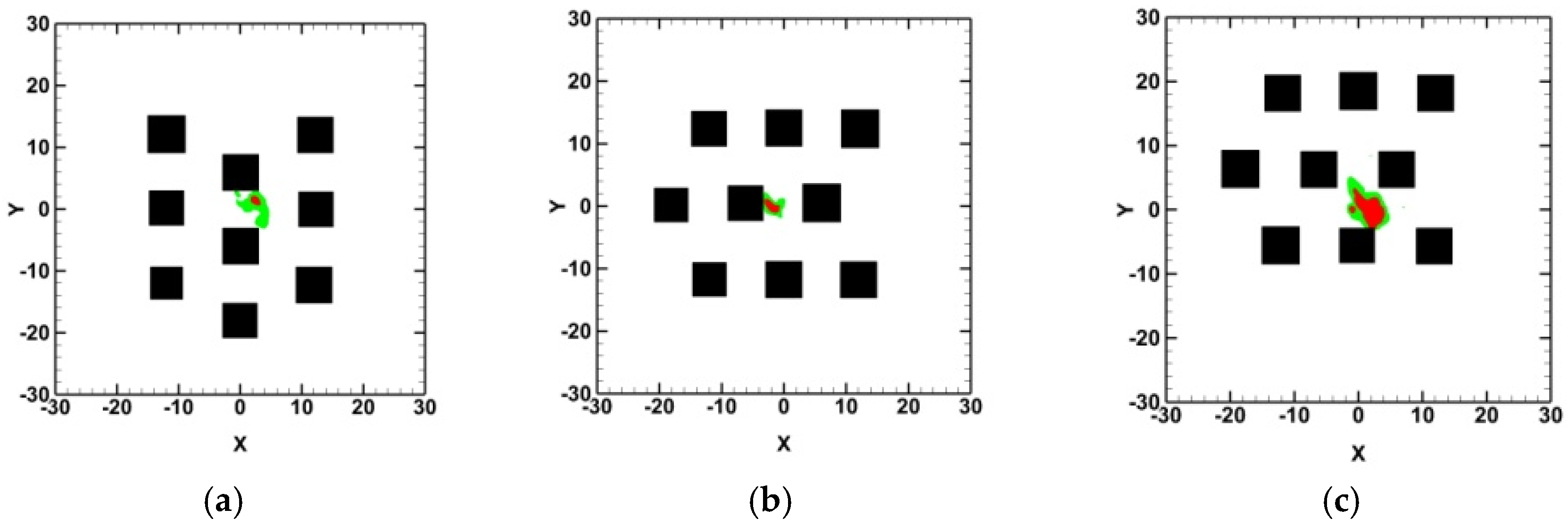
Figure 11 and
Figure 12 present the limits of the LC1 and IDLH zones for the three different cases after 200 s at the fire’s symmetry plane and a horizontal plane placed
Z = 1 m above the ground. The LC1 zone is indicated with the red color and the IDLH zone with the green color.
As is shown in
Figure 11a and
Figure 12a, the IDLH smoke zone dispersed towards the D2 cube. For this reason, all the cube’s façade openings of this side should be closed and protected in a street fire case. Most of the smoke products exited the street canyon before reaching the D2 cube. A wider distribution of the IDLH zone was presented between the C1 and E1 cubes. The non-symmetrical geometry had as an effect a wider distribution of the IDLH zone between the cubes. According to
Figure 11b and
Figure 12b, the IDLH smoke zone dispersed towards the leeward facade of the B2 cube. All the cube’s façade openings at this side should be closed and protected in a street fire case. Finally,
Figure 11c and
Figure 12c present the IDLH smoke zone from a fire incident that was not placed in a cube’s recirculation zone. The tilt of the IDLH smoke zone escaping the cube’s arrays height was similar for all the cases.
Table 1 defines the zone limits of the LC1 and IDLH zones for all the studied cases and for the Fire’s symmetry plane and a Horizontal Plane at
Z = 1 m above the ground. Case 2 presents the most extended area of the LC1 zone (4.2 m) at the Horizontal plane
Z = 1 m. Both Case 1 (1.35 m) and Case 3 (1.8 m) presented a similar LC1 zone extension. At the same plane, Case 3 presented the most extended area of the IDLH zone (5.83 m), and Case 1 (4.2 m) came after. At the fire’s symmetry plane, Case 3 presenteds the higher limits for both LC1 (2.5 m) and IDLH (23.32 m) zones. Concerning the LC1 zone, Case 1 presented the smallest radius extension of the 0.6 m radius, and Case 2 presented a 1.96 m radius extension. Finally, Case 1 presented an important IDLH radius extension of 18.5 m, and Case 2 presented a 10.4 m extension.
4. Conclusions
This study examined how a diesel pool fire incident affected the wind flow in a staggered array of cubes. The different urban geometry determinated the wind distribution and the smoke dispersion. Several predictions for the smoke dispersion and the fire accident position could be made for an urban area. Additionally, it defined the IDLH smoke zones for an incident occurring in a complex urban morphology and proposed the measurements for a quick response estimating the immediate intervention. The limits of the IDLH zones with contour graphs gave practical visual information for the danger zones and the definition of the intervention zones.
For a small distance between buildings and a perpendicular wind applied, a fire accident will direct the smoke towards the windward building. In a symmetrical geometry of urban blocks, the smoke after a fire accident will also be symmetrically dispersed. If the fire was between two buildings with a long distance, the smoke will be driven towards the leeward building. Complex geometries without any axis of symmetry could lead to unpredictable flows due to the fact that the wind may prefer to follow a specific path that could not be predicted with pre-planned actions. Finally, if the fire was placed in a road and the wind is parallel during the accident, the smoke followed the wind direction but was disturbed from the building’s lateral recirculation’s.
The LC1 and IDLH zone limits were calculated for all the cases. Street canyons, such as in Case 2, with small street width to building’s height ratio, presented the highest LC1 limits for the horizontal planes at 1 m height from the ground level. A pool fire that was placed in a well-ventilated position without a trap for the smoke pollutant presented an important extension of the IDLH zone along the wind direction.
Different wind velocities should be studied in order to define the possibility of the smoke re-entering back into the array’s cubes.
Author Contributions
Conceptualization, Konstantinos Vasilopoulos; Supervision, Panagiotis Tsoutsanis; Validation, Michalis Mentzos; Writing–original draft, Konstantinos Vasilopoulos; Writing–review & editing, Ioannis E. Sarris.
Funding
This research received no external funding.
Conflicts of Interest
The authors declare no conflicts of interest.
References
- Wood, C.R.; Arnold, S.J.; Balogun, A.A.; Barlow, J.F.; Belcher, S.E.; Britter, R.E.; Cheng, H.; Dobre, A.; Lingard, J.J.N.; Martin, D.; et al. Dispersion Experiments in Central London: The 2007 DAPPLE project. Bull. Am. Meteorol. Soc. 2009, 90, 955–970. [Google Scholar] [CrossRef] [Green Version]
- Dobre, A.; Arnold, S.J.; Smalley, R.; Boddy, J.W.D.; Barlow, J.; Tomlin, A.; Belcher, S.E. Flow field measurements in the proximity of an urban intersection in London, UK. Atmos. Environ. 2005, 39, 4647–4657. [Google Scholar] [CrossRef]
- Allwine, K.J.; Flaherty, J.E. Urban Dispersion Program MSG05 Field Study: Summary of Tracer and Meteorological Measurements; PNNL-15969; Pacific Northwest National Laboratory: Richland, WA, USA, 2006.
- García-Sánchez, C.; Van Tendeloo, G.; Gorlé, C. Quantifying inflow uncertainties in RANS simulations of urban pollutant dispersion. Atmos. Environ. 2017, 161, 263–273. [Google Scholar] [CrossRef]
- Markatos, N.C.; Malin, M.R.; Cox, G. Mathematical modelling of buoyancy-induced smoke flow in enclosures. Int. J. Heat Mass Transf. 1982, 25, 63–75. [Google Scholar] [CrossRef]
- Stavrakakis, G.M.; Markatos, N.C. Simulation of airflow in one- and two-room enclosures containing a fire source. Int. J. Heat Mass Transf. 2009, 52, 2690–2703. [Google Scholar] [CrossRef]
- Drikakis, D.; Rider, W. High-Resolution Methods for Incompressible and Low-Speed Flows; Springer: Berlin/Heidelberg, Germany, 2010. [Google Scholar]
- Drikakis, D. Advances in turbulent flow computations using high-resolution methods. Prog. Aerosp. Sci. 2003, 39, 405–424. [Google Scholar] [CrossRef] [Green Version]
- Ricci, A.; Burlando, M.; Freda, A.; Repetto, M.P. Wind tunnel measurements of the urban boundary layer development over a historical district in Italy. Build. Environ. 2017, 111, 192–206. [Google Scholar] [CrossRef]
- Coceal, O.; Goulart, E.V.; Branford, S.; Glyn Thomas, T.; Belcher, S.E. Flow structure and near-field dispersion in arrays of building-like obstacles. J. Wind Eng. Ind. Aerodyn. 2014, 125, 52–68. [Google Scholar] [CrossRef]
- Ramponi, R.; Blocken, B.; de Coo, L.B.; Janssen, W.D. CFD simulation of outdoor ventilation of generic urban configurations with different urban densities and equal and unequal street widths. Build. Environ. 2015, 92, 152–166. [Google Scholar] [CrossRef] [Green Version]
- DePaul, F.T.; Sheih, C.M. Measurements of wind velocities in a street canyon. Atmos. Environ. 1986, 20, 455–459. [Google Scholar] [CrossRef]
- Johnson, W.B.; Dabberdt, W.F.; Ludwig, F.L.; Allen, R.J. Field Study for Initial Evaluation of an Urban Diffusion Model for Carbon Monoxide; Comprehensive Report; Stanford Research Institute: Menlo Park, CA, USA, 1971; p. 144. [Google Scholar]
- Davidson, M.J.; Mylne, K.R.; Jones, C.D.; Phillips, J.C.; Perkins, R.J.; Fung, J.C.H.; Hunt, J.C.R. Plume dispersion through large groups of obstacles—A field investigation. Atmos. Environ. 1995, 29, 3245–3256. [Google Scholar] [CrossRef]
- Baik, J.-J.; Kim, J.-J. A Numerical Study of Flow and Pollutant Dispersion Characteristics in Urban Street Canyons. J. Appl. Meteorol. 1998, 98, 1576–1589. [Google Scholar] [CrossRef]
- Kim, J.-J.; Baik, J.-J. Effects of inflow turbulence intensity on flow and pollutant dispersion in an urban street canyon. J. Wind Eng. Ind. Aerodyn. 2003, 91, 309–329. [Google Scholar] [CrossRef]
- Hunter, L.J.; Johnson, G.T.; Watson, I.D. An investigation of three-dimensional characteristics of flow regimes within the urban canyon. Atmos. Environ. Part B Urban Atmos. 1992, 26, 425–432. [Google Scholar] [CrossRef]
- Johnson, W.B.; Ludwig, F.L.; Dabberdt, W.F.; Allen, R.J. An Urban Diffusion Simulation Model For Carbon Monoxide. J. Air Pollut. Control. Assoc. 1973, 23, 490–498. [Google Scholar] [CrossRef] [PubMed] [Green Version]
- Dabberdt, W.F.; Ludwig, F.L.; Johnson, W.B. Validation and applications of an urban diffusion model for vehicular pollutants. Atmos. Environ. 1973, 7, 603–618. [Google Scholar] [CrossRef]
- Liu, C.-H.; Wong, C.C.C. On the pollutant removal, dispersion, and entrainment over two-dimensional idealized street canyons. Atmos. Res. 2014, 135–136, 128–142. [Google Scholar] [CrossRef]
- Hu, L.H.; Huo, R.; Yang, D. Large eddy simulation of fire-induced buoyancy driven plume dispersion in an urban street canyon under perpendicular wind flow. J. Hazard. Mater. 2009, 166, 394–406. [Google Scholar] [CrossRef]
- Soulhac, L.; Garbero, V.; Salizzoni, P.; Mejean, P.; Perkins, R.J. Flow and dispersion in street intersections. Atmos. Environ. 2009, 43, 2981–2996. [Google Scholar] [CrossRef]
- Hoydysh, W.G.; Dabberdt, W.F. Concentration fields at urban intersections: fluid modeling studies. Atmos. Environ. 1994, 28, 1849–1860. [Google Scholar] [CrossRef]
- Dabberdt, W.; Hoydysh, W.; Schorling, M.; Yang, F.; Holynskyj, O. Dispersion modeling at urban intersections. Sci. Total. Environ. 1995, 169, 93–102. [Google Scholar] [CrossRef]
- Heath, T.; Smith, S.G.; Lim, B. Tall Buildings and the Urban Skyline:The Effect of Visual Complexity on Preferences. Environ. Behav. 2000, 32, 541–556. [Google Scholar] [CrossRef]
- Aristodemou, E.; Boganegra, L.M.; Mottet, L.; Pavlidis, D.; Constantinou, A.; Pain, C.; Robins, A.; ApSimon, H. How tall buildings affect turbulent air flows and dispersion of pollution within a neighbourhood. Environ. Pollut. 2018, 233, 782–796. [Google Scholar] [CrossRef] [PubMed]
- Xing, Y.; Brimblecombe, P. Dispersion of traffic derived air pollutants into urban parks. Sci. Total. Environ. 2018, 622–623, 576–583. [Google Scholar] [CrossRef] [PubMed]
- Davidson, M.J.; Snyder, W.H.; Lawson, R.E., Jr.; Hunt, J.C.R. Wind tunnel simulations of plume dispersion through groups of obstacles. Atmos. Environ. 1996, 30, 3715–3731. [Google Scholar] [CrossRef]
- Sudheer, S.; Kumar, L.; Manjunath, B.S.; Pasi, A.; Meenakshi, G.; Prabhu, S.V. Fire safety distances for open pool fires. Infrared Phys. Technol. 2013, 61, 265–273. [Google Scholar] [CrossRef]
- Vasanth, S.; Tauseef, S.M.; Abbasi, T.; Abbasi, S.A. Multiple pool fires: Occurrence, simulation, modeling and management. J. Loss Prev. Process. Ind. 2014, 29, 103–121. [Google Scholar] [CrossRef]
- Chatris, J.M.; Quintela, J.; Folch, J.; Planas, E.; Arnaldos, J.; Casal, J. Experimental study of burning rate in hydrocarbon pool fires. Combust. Flame 2001, 126, 1373–1383. [Google Scholar] [CrossRef]
- Jiang, P.; Lu, S.-X. Pool Fire Mass Burning Rate and Flame Tilt Angle under Crosswind in Open Space. Procedia Eng. 2016, 135, 261–274. [Google Scholar] [CrossRef]
- Argyropoulos, C.D.; Sideris, G.M.; Christolis, M.N.; Nivolianitou, Z.; Markatos, N.C. Modelling pollutants dispersion and plume rise from large hydrocarbon tank fires in neutrally stratified atmosphere. Atmos. Environ. 2010, 44, 803–813. [Google Scholar] [CrossRef]
- Argyropoulos, C.D.; Christolis, M.N.; Nivolianitou, Z.; Markatos, N.C. A hazards assessment methodology for large liquid hydrocarbon fuel tanks. J. Loss Prev. Process. Ind. 2012, 25, 329–335. [Google Scholar] [CrossRef]
- Markatos, N.C.; Christolis, C.; Argyropoulos, C. Mathematical modeling of toxic pollutants dispersion from large tank fires and assessment of acute effects for fire fighters. Int. J. Heat Mass Transf. 2009, 52, 4021–4030. [Google Scholar] [CrossRef]
- Baik, J.-J.; Kang, Y.-S.; Kim, J.-J. Modeling reactive pollutant dispersion in an urban street canyon. Atmos. Environ. 2007, 41, 934–949. [Google Scholar] [CrossRef]
- Kastner-Klein, P.; Plate, E.J. Wind-tunnel study of concentration fields in street canyons. Atmos. Environ. 1999, 33, 3973–3979. [Google Scholar] [CrossRef]
- Zhang, X.; Hu, L.; Tang, F.; Wang, Q. Large Eddy Simulation of Fire Smoke Re-circulation in Urban Street Canyons of Different Aspect Ratios. Procedia Eng. 2013, 62, 1007–1014. [Google Scholar] [CrossRef]
- Pesic, D.J.; Blagojevic, M.D.; Zivkovic, N.V. Simulation of wind-driven dispersion of fire pollutants in a street canyon using FDS. Environ. Sci. Pollut. Res. 2014, 21, 1270–1284. [Google Scholar] [CrossRef]
- Hu, L.H.; Xu, Y.; Zhu, W.; Wu, L.; Tang, F.; Lu, K.H. Large eddy simulation of pollutant gas dispersion with buoyancy ejected from building into an urban street canyon. J. Hazard. Mater. 2011, 192, 940–948. [Google Scholar] [CrossRef]
- Hu, L.; Zhang, X.; Zhu, W.; Ning, Z.; Tang, F. A global relation of fire smoke re-circulation behaviour in urban street canyons. J. Civ. Eng. Manag. 2015, 21, 459–469. [Google Scholar] [CrossRef]
- Pesic, D.J.; Zigar, D.N.; Anghel, I.; Glisovic, S.M. Large Eddy Simulation of wind flow impact on fire-induced indoor and outdoor air pollution in an idealized street canyon. J. Wind Eng. Ind. Aerodyn. 2016, 155, 89–99. [Google Scholar] [CrossRef]
- Inagaki, A.; Kanda, M. Turbulent flow similarity over an array of cubes in near-neutrally stratified atmospheric flow. J. Fluid Mech. 2008, 615, 101–120. [Google Scholar] [CrossRef]
- Shen, Z.; Wang, B.; Cui, G.; Zhang, Z. Flow pattern and pollutant dispersion over three dimensional building arrays. Atmos. Environ. 2015, 116, 202–215. [Google Scholar] [CrossRef]
- King, M.-F.; Gough, H.L.; Halios, C.; Barlow, J.F.; Robertson, A.; Hoxey, R.; Noakes, C.J. Investigating the influence of neighbouring structures on natural ventilation potential of a full-scale cubical building using time-dependent CFD. J. Wind Eng. Ind. Aerodyn. 2017, 169, 265–279. [Google Scholar] [CrossRef]
- Gough, H.; Sato, T.; Halios, C.; Grimmond, C.S.B.; Luo, Z.; Barlow, J.F.; Robertson, A.; Hoxey, R.; Quinn, A. Effects of variability of local winds on cross ventilation for a simplified building within a full-scale asymmetric array: Overview of the Silsoe field campaign. J. Wind Eng. Ind. Aerodyn. 2018, 175, 408–418. [Google Scholar] [CrossRef]
- McGrattan, K.; Baum, H.; Rehm, R.; Hamins, A.; Forney, G.; Floyd, J.; Hostikka, S.; Prasad, K. Fire Dynamics Simulator (Version 5) Technical Reference Guide; NIST Special Publication: Gaithersburg, MD, USA, 2010; Volume 1018. [Google Scholar]
- Grigoriadis, D.G.E.; Sarris, I.E.; Kassinos, S.C. MHD flow past a circular cylinder using the immersed boundary method. Comput. Fluids 2010, 39, 345–358. [Google Scholar] [CrossRef]
- Richards, P.J.; Hoxey, R.P. Appropriate boundary conditions for computational wind engineering models using the k-ϵ turbulence model. J. Wind Eng. Ind. Aerodyn. 1993, 46–47, 145–153. [Google Scholar] [CrossRef]
- Richards, P.J.; Hoxey, R.P.; Short, J.L. Spectral models for the neutral atmospheric surface layer. J. Wind Eng. Ind. Aerodyn. 2000, 87, 167–185. [Google Scholar] [CrossRef]
- Babrauskas, V. Estimating large pool fire burning rates. Fire Technol. 1983, 19, 251–261. [Google Scholar] [CrossRef]
- Walton, W.D.; Twilley, W.H.; Putorti, A.D.; Hiltabrand, R.R. Smoke measurements using an advanced helicopter transported sampling package with radio telemetry. In Proceedings of the 18th Arctic and Marine Oilspill Program (AMOP) Technical Seminar, Environment, Ottawa, ON, Canada, 14–16 June 1995; pp. 1053–1074. [Google Scholar]
- Assael, M.J.; Kakosimos, K.E. Fires, Explosions, and Toxic Gas Dispersions: Effects Calculation and Risk Analysis; CRC Press: Boca Raton, FL, USA, 2010. [Google Scholar]
© 2018 by the authors. Licensee MDPI, Basel, Switzerland. This article is an open access article distributed under the terms and conditions of the Creative Commons Attribution (CC BY) license (http://creativecommons.org/licenses/by/4.0/).

 ,
, 


