On Parameter Estimation for Bandlimited Optical Intensity Channels

Abstract

Parameter estimation is of paramount importance in every digital receiver. This is not only true for radio, but also for optical links; otherwise, subsequent processing stages, like detector units or error correction schemes, could not be operated reliably. However, for a bandlimited optical intensity channel, the problem of parameter estimation is strongly related to non-negative pulse shapes satisfying also the Nyquist criterion to keep the detection process as simple as possible. To the best of the author’s knowledge, it is the first time that both topics—parameter estimation on the one hand and bandlimited intensity modulation on the other—are jointly investigated. Since symbol timing and signal amplitude are the parameters of interest in this case, the corresponding Cramer–Rao lower bounds are derived as the theoretical limit of the jitter variance generated by the related estimator algorithms. In this context, a maximum likelihood solution is developed for the recovery of both timing and amplitude. Since this approach requires a receiver matched filter destroying the Nyquist criterion of the non-negative pulse shape, we compare it to a flat receiver filter preserving the required orthogonality property. It turned out that the jitter performance of the matched filter method is close to the Cramer–Rao lower bound in the medium-to-low SNR range, but due to inter-symbol interference effects an error floor emerges at higher SNR values. The flat filter solution avoids this drawback, although the price to be paid is a larger noise level at the filter output, so that a somewhat increased jitter variance is observed.

1. Introduction

There is no doubt that optical wireless communication (OWC) systems have some remarkable benefits compared to radio frequency (RF) solutions [1,2,3,4]: no regulatory and license problems, rapid deployment and inexpensive operation, as well as data security and throughput, just to cite briefly the most important aspects. However, even for OWC links, the available bandwidth is not infinite, but subject to limitations because of different reasons, e.g., physical restrictions of electrical and optical elements in transmitters and receivers, dispersion effects introduced by the channel, or impairments due to multipath propagation in indoor applications. For an optical intensity link [5], this means that the baseband pulse has to be shaped appropriately in the transmitter unit to avoid negative signal components. On the other hand, it is still appreciated that the waveform satisfies the Nyquist criterion in order to keep the detection process in the receiver module as simple as possible.

For a bandlimited OWC link, characterized by intensity modulation and direct detection (IM/DD), it was shown in [6] that both the non-negativity and Nyquist requirements are satisfied for a squared sinc pulse; for practical reasons admitting some amount of excess bandwidth, this results in a squared raised cosine (SRC) function. It was proved in [6] as well that a suitable root-Nyquist solution does not exist in the context of limited bandwidth, although this would be necessary to implement a matched filter (MF) in the receiver station to maximize the signal-to-noise ratio (SNR) at the detector output. As an alternative, the authors in [7,8] suggested that the non-negativity constraint is achieved by an offset component, although this is less efficient in terms of power, but it needs only half of the bandwidth compared to an SRC approach. Finally, a two-dimensional signal space was studied in [9,10] to increase the spectral efficiency of optical links.

Powerful estimation of the most important transmission parameters is key for any receiver terminal [11,12], which does not only hold true for radio, but also for optical scenarios. Regarding the latter, knowledge of both symbol timing and signal amplitude is of paramount importance; otherwise, subsequent stages, like detector units or error correction schemes, cannot be operated reliably. Scanning the open literature in this context, numerous contributions about channel estimation and/or symbol timing recovery are available, but they are not or only marginally related to bandwidth constraints and pulse shaping. From the author’s point of view, it is the first time that this specific problem is analyzed and discussed in a structured and non-heuristic manner for the current contribution.

The remainder of the paper is organized as follows: The signal and channel model used for analytical and simulation work is introduced in Section 2. In Section 3, we derive the Cramer–Rao lower bound as the theoretical limit of the error performance. Next, a maximum likelihood estimator is developed in Section 4; since this requires a receiver MF violating the Nyquist property, a modified solution is investigated based on the implementation of a flat receiver filter. Numerical results are presented in Section 5, and Section 6 concludes the paper.

2. Signal and Channel Model

In the sequel, we assume that the real-valued data symbols a_k, $k\in \mathbb{Z}$, are independent and identically distributed (i.i.d.) elements of an M-ary pulse amplitude modulation (PAM) alphabet $\mathrm{A}$. For convenience reasons, the alphabet is organized such that the symbols are normalized to unit energy, i.e., a_k ∈ $\mathrm{A}$ = $\{0,1,\dots ,M-1\}/\sqrt{{\eta }_M}$, where ${\eta }_M=\frac{1}{6}(M-1)(2M-1)$. This means that the average value is given by

$${\mu }_a=\frac{M-1}{2\sqrt{{\eta }_M}}=\sqrt{\frac{3(M-1)}{2(2M-1)}}.$$

(1)

Furthermore, it is assumed that the pulses in the transmitter station are either shaped by a squared raised cosine (SRC) or a squared double jump (SDJ) function [6] specified as

$$h(t)=\frac{1}{\sqrt{T}}\{\begin{array}{l}{\left(\sin \mathrm{c}(t/T)\frac{\cos (\pi \alpha t/T)}{1-{(2\alpha t/T)}^2}\right)}^2\dots \mathrm{SRC}\\ {\left(\frac{1-\alpha }{2}\sin \mathrm{c}[(1-\alpha )t/T]+\frac{1+\alpha }{2}\sin \mathrm{c}[(1+\alpha )t/T]\right)}^2\dots \mathrm{SDJ}\end{array}$$

(2)

where sinc(x) = sin(πx)/(πx), 0 ≤ α ≤ 1 is the excess bandwidth (roll-off factor), and T stands for the symbol period the OWC link is operated with.

Note that SRC and SDJ shapes satisfy both the non-negativity and the Nyquist criteria, exemplified in Figure 1 for α ∈ {0.0, 0.5, 1.0}. Note also that SRC and SDJ are equivalent for α = 0, which represents the minimum bandwidth (MBW) case. By detailed inspection of the plot, we observe that the width of the main lobe decreases when α is increased and that this effect is more pronounced for SDJ scenarios.

No matter which sort of pulse shape is finally implemented, the generated transmitter signal can be written as

$$s(t)={\displaystyle \sum _k{a}_{k}h(t-kT)}.$$

(3)

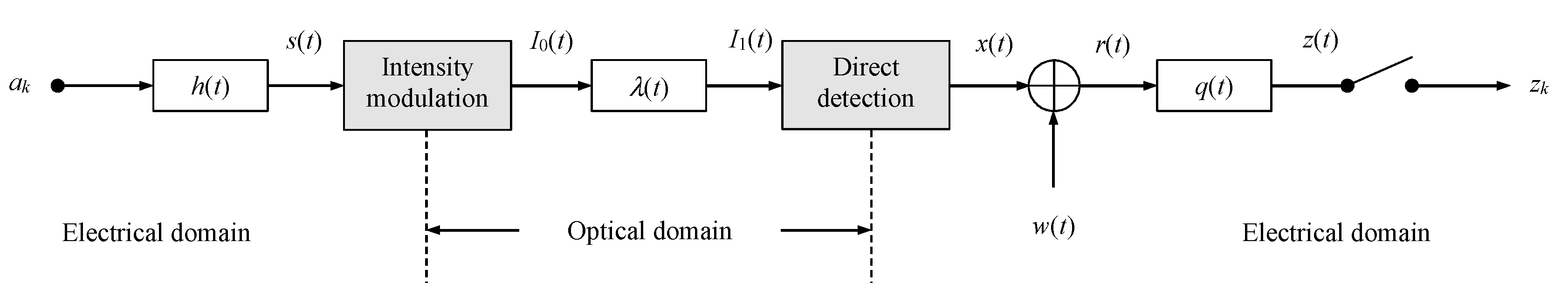
By introduction of the electro–optical conversion factor K₀, the irradiated signal at the output of the intensity modulator is given as I₀(t) = K₀ s(t). If we adopt an observation window for the estimation procedure, which is small enough so that the channel state does not change significantly over this period of time, then fading effects need not be taken into account. This means that the optical signal of interest at the receiver is only affected by some propagation loss and a delay in time, henceforth denoted by K_l and τ, respectively; as a result, the transfer function of the channel is obtained as λ(t) = K_l δ(t – τ), where δ(⋅) symbolizes Dirac’s delta function. Therefore, the optical signal intensity at the input of the receiver terminal is simply described as I₁(t) = λ(t) ⊗ I₀(t) = K_l K₀ s(t – τ), where ⊗ denotes the convolutional operator. Specifying in the sequel the detector responsivity as R_d, the electrical signal at the detector output is determined by x(t) = R_d I₁(t) = A⋅s(t – τ), where A = R_d K_l K₀ is the gain factor characterizing the OWC link. Finally, we have to consider that x(t) is distorted by additive white Gaussian noise (AWGN), in the following denoted as w(t), with zero mean and variance ${\sigma }_w^2$. Putting these pieces together, the receiver signal can be expressed as

$$r(t)=x(t)+w(t)=A\cdot s(t-\tau )+w(t).$$

(4)

However, before being treated in further stages of operation, the signal in (4) has to pass the receiver filter q(t), whose output z(t) = q(t) ⊗ r(t) is appropriately sampled to avoid alias effects. For convenience reasons, the signal and channel model used for analytical and simulation work is summarized in Figure 2.

Before we proceed to the computation of the Cramer–Rao lower bound in the next section, it makes sense to introduce the average optical power as $P_0={\mu }_a\overline{h}$, where

$$\overline{h}=\frac{1}{\sqrt{T}}{\displaystyle \underset{-\infty }{\overset{\infty }{\int }}h(t)dt}=\{\begin{array}{l}1-\frac{\alpha }{4}\dots \mathrm{SRC}\\ 1-\frac{\alpha }{2}\dots \mathrm{SDJ}\end{array}$$

(5)

In addition, the average electrical SNR at the receiver is defined as

$${\gamma }_s=\frac{A^2{P}_0^2}{{\sigma }_w^2}.$$

(6)

It has been proved in [6] that the SDJ pulse is optimal insofar as $\overline{h}$ achieves a minimum for a given value of α, which is a major motivation to compare the performance of this kind of pulse to SRC shapes.

3. Modified Cramer–Rao Lower Bound

3.1. Derivation of the Log-Likelihood Function

The jitter (error) variance of a parameter estimator is a main figure of merit, which is benchmarked by the Cramer–Rao lower bound (CRLB) as the theoretical limit [11,13]. As already mentioned in the introductory section, little or no information about this topic could be found in the open literature when it comes to the estimation of signal amplitudes and symbol timing for bandlimited OWC links [14].

According to the signal model specified previously, we are considering a parameter vector u = (u₁, u₂) = (A, τ). Furthermore, we are assuming a data-aided (DA) situation, i.e., the estimation process is based on the knowledge of L data symbols a_k forming a preamble or pilot sequence, where $k\in \mathrm{K}=\{k_0,k_0+1,\dots ,k_0+L-1\}$. Then, if r describes the vector representation of (4) over an observation window of L symbol periods, the CRLB is for unbiased estimation of parameter u_m given by

$$\mathrm{CRLB}(u_m)={[J^{-1}(u)]}_m,$$

(7)

with [⋅]_m indicating the m-th diagonal entry of the inverted Fisher information matrix (FIM) expressed by J(u). For row m and column n, the FIM element is formally evaluated as

$$J_{m,n}\equiv {[J(u)]}_{m,n}=-\mathrm{E}\left[\frac{{\partial }^2\mathsf{\Lambda }(r;u)}{\partial u_m\partial u_n}\right],$$

(8)

where Λ(r;u) is the log-likelihood function (LLF) for the L observables in r, and $\mathrm{E}[\cdot ]$ denotes expectation with respect to the AWGN process.

By detailed inspection of (8), it is clear that the knowledge of the LLF is mandatory for the computation of the CRLB. Nevertheless, if we keep in mind that r(t) is a white Gaussian process, then the LLF is immediately provided by

$$\begin{array}{ll}\mathsf{\Lambda }(r;u)& =-\frac{1}{2{\sigma }_w^2}{\displaystyle \underset{-\infty }{\overset{+\infty }{\int }}{[r(t)-A\cdot s(t-\tau )]}^{2}dt}\\ & ~\frac{1}{2{\sigma }_w^2}{\displaystyle \underset{-\infty }{\overset{+\infty }{\int }}\{2A\cdot r(t)s(t-\tau )-{[A\cdot s(t-\tau )]}^2\}dt}.\end{array}$$

(9)

Note that immaterial constants and factors not depending on u are already omitted in (9). Next, we introduce the definition

$$z_k={\displaystyle \underset{-\infty }{\overset{+\infty }{\int }}r(t)h(t-kT-\tau )dt},$$

(10)

which determines the output of a filter with impulse response h(–t) evaluated at t = kT + τ and fed with r(t). By detailed inspection of Figure 2, it becomes obvious that this filter is exactly the receiver MF specified by q(t) = h(–t); for SRC and SDJ shapes, it is clear that h(t) = h(–t). Moreover, we have

$$\begin{array}{ll}{\displaystyle \underset{-\infty }{\overset{+\infty }{\int }}{[s(t-\tau )]}^{2}dt}& ={\displaystyle \sum _{k\in \mathrm{K}}{\displaystyle \sum _{n\in K}{a}_k{a}_n{\displaystyle \underset{-\infty }{\overset{+\infty }{\int }}h(t-kT-\tau )h(t-nT-\tau )dt}}}\\ & ={\displaystyle \sum _{k\in \mathrm{K}}{\displaystyle \sum _{n\in \mathrm{K}}{a}_k{a}_{n}g[(k-n)T]},}\end{array}$$

(11)

where g(t) = h(t) ⊗ h(–t). Finally, by plugging (10) and (11) into (9), the LLF of our estimation problem is established as

$$\mathsf{\Lambda }(r;u)=\frac{1}{2{\sigma }_w^2}\left(2A{\displaystyle \sum _{k\in \mathrm{K}}{a}_k{z}_k-A^2{\displaystyle \sum _{k\in \mathrm{K}}{\displaystyle \sum _{n\in \mathrm{K}}{a}_k{a}_{n}g[(k-n)T]}}}\right).$$

(12)

3.2. Computation of the Modified CRLB

Using the LLF in (12), the FIM elements can be computed according to (8). Since we need not consider any nuisance parameters, the expectation is for a DA solution only with regard to the AWGN process. As a consequence, the entries would be a function of the selected synchronization sequence a_k with $k\in \mathrm{K}$. In the sequel, we want to circumvent this sort of dependency by averaging the second-order derivative in (8) not only with respect to w(t), but also with respect to the i.i.d. symbols $a_k\in \mathrm{A}$. This provides us with the so-called modified Cramer–Rao lower bound (MCRLB), which is in general less tight than the true limit [15,16,17,18], i.e., MCRLB(u_m) ≤ CRLB(u_m).

In the next step, the FIM elements J_m,n will be derived for all m, n ∈ {1, 2}. Starting with u₁ = u₂ = A, we obtain

$$\begin{array}{ll}{J}_{1,1}& =-\mathrm{E}\left[\frac{{\partial }^2\mathsf{\Lambda }(r;u)}{\partial A^2}\right]\\ & =\frac{1}{{\sigma }_w^2}{\displaystyle \sum _k{\displaystyle \sum _n\mathrm{E}[a_k{a}_n]}}g[(k-n)T]\\ & =\frac{1}{{\sigma }_w^2}\left\{{\displaystyle \sum _k\mathrm{E}[a_k^2]}g(0)+2{\displaystyle \sum _k{\displaystyle \sum _{n>k}\mathrm{E}[a_k]\mathrm{E}[a_n]}}g[(k-n)T]\right\}\\ & =\frac{1}{{\sigma }_w^2}\left\{Lg(0)+2{\mu }_a^2{\displaystyle \sum _{i=1}^{L-1}(L-i)g(iT)}\right\},\end{array}$$

(13)

where, for notational brevity, it has been tacitly assumed that the summation indexes k and n are elements of $\mathrm{K}$. Then, with u₁ = A, u₂ = τ, and $\dot{h}(t)=\partial h(t)/\partial t$, the related FIM element is given by

$$\begin{array}{ll}{J}_{1,2}& =-\mathrm{E}\left[\frac{{\partial }^2\mathsf{\Lambda }(r;u)}{\partial A\partial \tau }\right]\\ & =\frac{A^2}{{\sigma }_w^2}{\displaystyle \sum _k{\displaystyle \sum _n\mathrm{E}[a_k{a}_n]}}{\displaystyle \underset{-\infty }{\overset{\infty }{\int }}\dot{h}(t-kT-\tau )h(t-nT-\tau )dt}\\ & =\frac{A^2}{{\sigma }_w^2}{\displaystyle \sum _k{\displaystyle \sum _n\mathrm{E}[a_k{a}_n]}}\dot{g}[(k-n)T]=0,\end{array}$$

(14)

where we used the fact that the integral in (14) is equivalent to the first-order derivative of g(t), expressed as $\dot{g}(t)$, which has to be evaluated at integer multiples of the symbol period within the index range determined by the observation interval. Since $\dot{g}(t)$ exhibits an odd symmetry with respect to t = 0, it is not difficult to show that J_1,2 = 0. Since the LLF is a steadily differentiable function with respect to u₁ and u₂, it is clear that J_2,1 = J_1,2 = 0.

Finally, with u₁ = u₂ = τ and $\ddot{h}(t)={\partial }^{2}h(t)/\partial t^2$, the corresponding FIM element develops as

$$\begin{array}{ll}{J}_{2,2}& =-\mathrm{E}\left[\frac{{\partial }^2\mathsf{\Lambda }(r;u)}{\partial {\tau }^2}\right]\\ & =-\frac{A^2}{{\sigma }_w^2}{\displaystyle \sum _k{\displaystyle \sum _n\mathrm{E}[a_k{a}_n]}}{\displaystyle \underset{-\infty }{\overset{\infty }{\int }}\ddot{h}(t-kT-\tau )h(t-nT-\tau )dt}\\ & =-\frac{A^2}{{\sigma }_w^2}{\displaystyle \sum _k{\displaystyle \sum _n\mathrm{E}[a_k{a}_n]}}\ddot{g}[(k-n)T]\\ & =-\frac{A^2}{{\sigma }_w^2}\left\{L\ddot{g}(0)+2{\mu }_a^2{\displaystyle \sum _{i=1}^{L-1}(L-i)\ddot{g}(iT)}\right\},\end{array}$$

(15)

after having exploited the fact that the integral expression in (15) describes the second-order derivative of g(t), denoted as $\ddot{g}(t)$, which has to be evaluated at integer multiples of the symbol period for all k and $n\in \mathrm{K}$. Taking into account that $\ddot{g}(t)$ is even–symmetric, the simplification in the last line of (15) is achieved straightforwardly.

According to (7), it is obvious that the MCRLB of parameter u_m is solely determined by the reciprocal value of J_m,m, when the off-diagonal entries are zero. Therefore, regarding the signal amplitude, we have

$$\mathrm{MCRLB}(A)=\frac{1}{J_{1,1}}=\frac{A^2{P}_0^2}{L{\gamma }_s\left\{g(0)+2{\mu }_a^2{\displaystyle \sum _{i=1}^{L-1}(1-\frac{i}{L})g(iT)}\right\}},$$

(16)

whereas for recovery of the symbol timing, the theoretical limit develops as

$$\mathrm{MCRLB}(\tau )=\frac{1}{J_{2,2}}=-\frac{P_0^2}{L{\gamma }_s\left\{\ddot{g}(0)+2{\mu }_a^2{\displaystyle \sum _{i=1}^{L-1}(1-\frac{i}{L})\ddot{g}(iT)}\right\}}.$$

(17)

To the best of the author’s knowledge, it is the first time that the MCRLB has been derived for a PAM constellation and a pulse shaping governed by an SRC or SDJ function, as it would be needed for a bandlimited optical intensity link. It is to be noticed that (16) and (17) apply in the same way to SRC as well as SDJ pulses. Finally, we recall that μ_a = 0 for zero-mean symbol alphabets like M-ary phase shift keying (PSK) or quadrature amplitude modulation (QAM) schemes; taking this into account, together with P₀ = 1 and g(t) as a simple raised cosine function, the relationships characterize the conditions for an RF link [11].

4. Estimator Algorithms

4.1. Maximum Likelihood Approach

Based on the LLF in (12), a maximum likelihood algorithm for joint estimation of signal amplitude and symbol timing might be achieved by setting the first-order derivatives ∂Λ(r;u)/∂u_m to zero and solving the (nonlinear) set of equations with respect to u_m. Needless to say, there exists no closed-form solution so that we must resort to a numerical procedure, e.g., the Newton–Raphson algorithm [19]. However, this iterative approach suffers normally from serious convergence and stability problems so that we present in the sequel a stable and much less complex method [20].

By detailed inspection of (12), it makes sense to skip the second term in parentheses, if we are interested in the estimation of the symbol timing, as this term does not depend on τ. With this simplification in mind, the corresponding LLF boils down to

$$\mathsf{\Lambda }(r;\tau )={\displaystyle \sum _{k=0}^{L-1}{\omega }_k{z}_k}={\displaystyle \underset{-\infty }{\overset{\infty }{\int }}\mathrm{\Omega }(t)r(t+\tau )dt},$$

(18)

where, for reasons of clarity, the synchronization symbols used in this context have been introduced as ω_k, and

$$\mathrm{\Omega }(t)={\displaystyle \sum _{k=0}^{L-1}{\omega }_{k}h(t-kT)}$$

(19)

represents a filter employed for the correlation procedure expressed by (18). Without loss of generality, it has been assumed for (18) and (19) that the index range $\mathrm{K}$ of the observation window starts with k₀ = 0. The estimate for symbol timing is then obtained as

$$\widehat{\tau }=\arg \underset{\tilde{\tau }}{\max }\mathsf{\Lambda }(r;\tilde{\tau }).$$

(20)

No closed-form solution is available to tackle the optimization problem in (20), so we have to envisage a numerical approach. To this end, we first discretize the involved timing parameters as follows: t → iT_s and $\tilde{\tau }$ → μT_s, i and $\mu \in \mathbb{Z}$, with T_s as the sampling interval specified as T_s = T/N_s; in order to avoid alias problems, it is necessary that the oversampling factor N_s selected is large enough. As a result, the function to be optimized for symbol timing recovery is introduced as

$${\mathsf{\Lambda }}_{\mu }={\displaystyle \sum _{i\in \mathrm{I}}\mathrm{\Omega }(i{T}_s)r[(i+\mu )T_s]}.$$

(21)

The range $\mathrm{I}$ in (21) is chosen such that the amplitude of Λ_μ drops below a certain limit, say 10^–6 or less, if the sampling index i is picked outside this range. Then the maximization process in (20) is elegantly re-formulated as

$$\widehat{\mu }=\arg \underset{\mu }{\max }{\mathsf{\Lambda }}_{\mu }.$$

(22)

The computational complexity of the optimization procedure relates to the granularity of the sampling grid determined by T_s, i.e., the smaller the value of T_s, the larger the computational load, and vice versa. A good compromise is the use of a medium kind of granularity and the extraction of values in between by an interpolation function. Simulation results have shown that a parabolic approach is sufficient (linear interpolation is too coarse to achieve reliable results, but orders larger than two require more computing resources and might cause oscillation problems). Hence, timing estimates are basically calculated via

$$\widehat{\tau }=\left(\widehat{\mu }-\frac{1}{2}\frac{{\mathsf{\Lambda }}_{\widehat{\mu }+1}-{\mathsf{\Lambda }}_{\widehat{\mu }-1}}{{\mathsf{\Lambda }}_{\widehat{\mu }+1}-2{\mathsf{\Lambda }}_{\widehat{\mu }}+{\mathsf{\Lambda }}_{\widehat{\mu }-1}}\right)T_s.$$

(23)

In the next stage of operation, we are going to extract the estimation of the signal amplitude. Conditioned on the knowledge that the timing estimate has been achieved previously, the derivative of the LLF in (12) gives

$${\frac{\partial \mathsf{\Lambda }(r;A,\widehat{\tau })}{\partial A}|}_{A=\widehat{A}}=2{\displaystyle \sum _{k=0}^{L-1}{\omega }_k{\widehat{z}}_k}-2\widehat{A}{\displaystyle \sum _{k=0}^{L-1}{\displaystyle \sum _{n=0}^{L-1}{\omega }_k{\omega }_{n}g[(k-n)T]}},$$

(24)

where ${\widehat{z}}_k$ denotes the output of the receiver MF according to (10), but now processed at $t=kT+\widehat{\tau }$. Setting (24) to zero, the signal amplitude is then estimated by

$$\begin{array}{ll}\widehat{A}& =\frac{{\displaystyle \sum _{k=0}^{L-1}{\omega }_k{\widehat{z}}_k}}{{\displaystyle \sum _{k=0}^{L-1}{\displaystyle \sum _{n=0}^{L-1}{\omega }_k{\omega }_{n}g[(k-n)T]}}}\\ & =\frac{{\mathsf{\Lambda }}_{\widehat{\mu }}}{g(0){\displaystyle \sum _{k=0}^{L-1}{\omega }_k^2}+2{\displaystyle \sum _{k=0}^{L-1}{\displaystyle \sum _{n=k+1}^{L-1}{\omega }_k{\omega }_{n}g[(k-n)T]}}}.\end{array}$$

(25)

In order to reduce the computational complexity of (25), the even–symmetric property of g(t) has been exploited in the denominator, whereas the numerator is just the correlation result in (21) evaluated at $\mu =\widehat{\mu }$. Finally, it is to be mentioned that the framework is still the same, no matter whether the optical link is operated with SRC or SDJ pulses.

4.2. Flat Receiver Filter

It is to be recalled that the estimators in Section 4.1 utilize a receiver MF specified by q(t) = h(t), which means that the Nyquist criterion will be violated at the MF output. In consequence, a more complicated detection process would be necessary to circumvent a degradation of the performance by inter-symbol interference (ISI) effects. Since a real-valued root-Nyquist function does not exist for bandlimited intensity links [6], we will explore a solution based on a flat receiver filter preserving the required orthogonality.

In particular, it is suggested that the receiver MF is substituted by a filter exhibiting a rectangular shape in the frequency domain occupying the same bandwidth as the user signal in (3), which is determined by $2(1+\alpha )/T$. Therefore, the corresponding impulse response develops as

$$q(t)=\frac{2(1+\alpha )}{\sqrt{T}}\sin \mathrm{c}[2(1+\alpha )t/T],$$

(26)

which means that $g(t)=h(t)\otimes q(t)=\sqrt{T}h(t)$, i.e., the Nyquist property is not violated.

With respect to the timing estimator developed before, this requires only the correlation filter in (19) to be modified insofar as h(t) is replaced by (26). On the other hand, the algorithm for estimating the amplitude in (25) simplifies significantly, because g(0) = 1 and g[(n – k)T] = 0 for all n ≠ k, which yields

$$\widehat{A}=\frac{{\mathsf{\Lambda }}_{\widehat{\mu }}}{{\displaystyle \sum _{k=0}^{L-1}{\omega }_k^2}}.$$

(27)

Nevertheless, the price to be paid for this approach is that the noise component at the output of the flat receiver filter increases compared to MF solutions. As a result, the jitter variance degrades somewhat, but it exhibits no error floor.

5. Numerical Results

In the sequel, the mean estimator value (MEV) and the jitter (error) variance are discussed as the main figures of merit, when it comes to the estimation of a transmission parameter u_m. The former is defined as the average value of the estimates generated by the algorithm selected for this purpose. From a practical point of view, it is most helpful if this is achieved without bias, i.e., $u_m=\mathrm{E}[{\widehat{u}}_m]$. On the other hand, for an efficient recovery algorithm, the related jitter variance should be as close to the MCRLB as possible.

For reasons of clarity and readability, analytical and simulation results will be indicated by lines and markers in different styles. Moreover, if not stated otherwise, the following parameterization is employed:

• The observation window consists of L = 100 symbol periods.
• We focus on the investigation of 4-PAM constellations, but the basic findings apply to M-ary PAM signals in general.
• The excess bandwidth of SRC or SDJ shapes is given by α ∈ {0.0, 0.5, 1.0}.
• An oversampling factor N_s = 4 is selected; this avoids alias effects and keeps the computational load as small as possible. However, it turned out that this might be problematic for larger values of the excess bandwidth, because in this case the main lobe of the pulse shape becomes smaller (see Figure 1) so that it is not resolved fine enough; this results in a bias effect for timing estimates, as could be verified by simulation results. Hence, for values of α ≥ 0.5, it is suggested to apply N_s = 8 for SRC as well as SDJ shapes.
• For convenience reasons, the timing offsets τ and amplitude gains A are normalized to the nominal values of symbol period and signal amplitude, T₀ and A₀, respectively, as such they will be denoted by ε = τ/T₀ and ρ = A/A₀.
• Results achieved by a matched filter or a flat filter receiver are indicated by MF and FF, respectively.

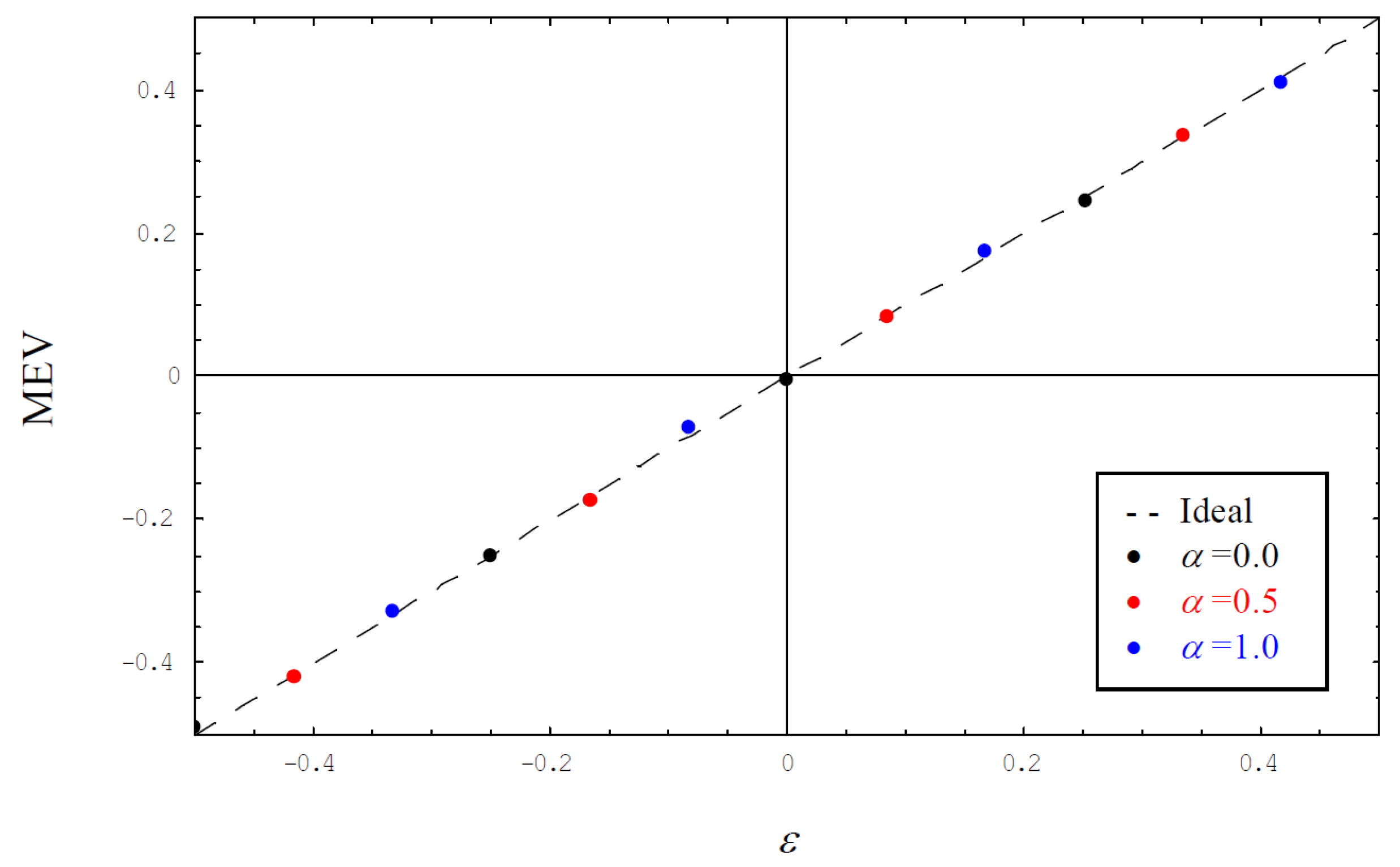
Assuming a reference index μ = 0 for symbol timing recovery in the range of the normalized symbol period, i.e., |ε | ≤ 1/2, Figure 3 shows the MEV for different values of the roll-off factor applied to SRC shapes using an MF receiver. We can see that the estimator exhibits no bias, indicated by the ideal curve in dashed style. Although not shown in Figure 3 to avoid an overload of the diagram, it could be verified that this also holds true for an FF receiver or if pulses are shaped by an SDJ function.

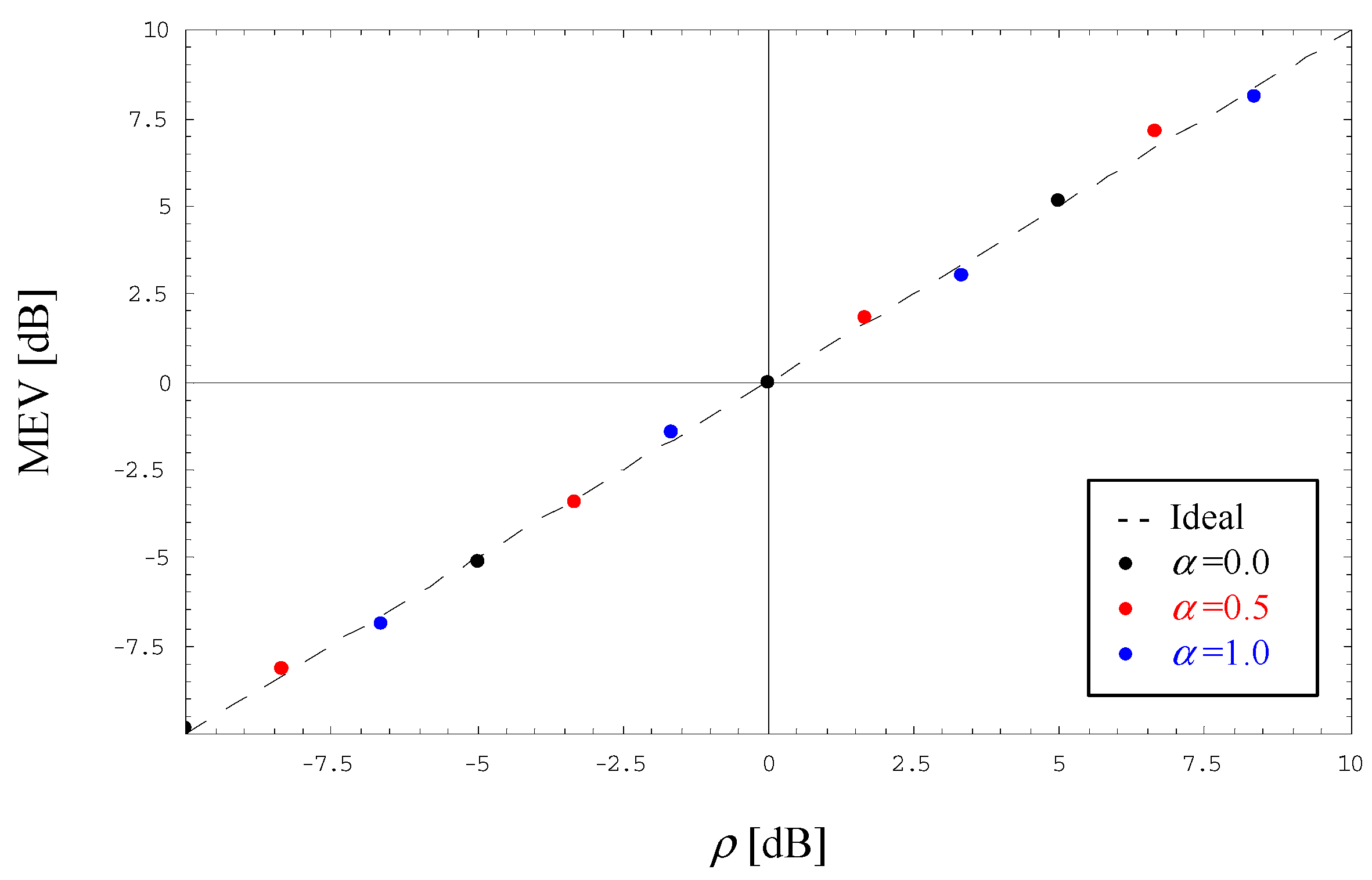
Of course, the algorithm for estimating the signal amplitude has been tested as well. Figure 4 illustrates the MEV of the normalized amplitude estimate delivered by (27) in the range of ±10 dB for an FF scenario applied to SDJ shapes and different values of α. Again, we observe that the estimation procedure is bias-free, which has also been tested for an MF scenario and SRC shapes.

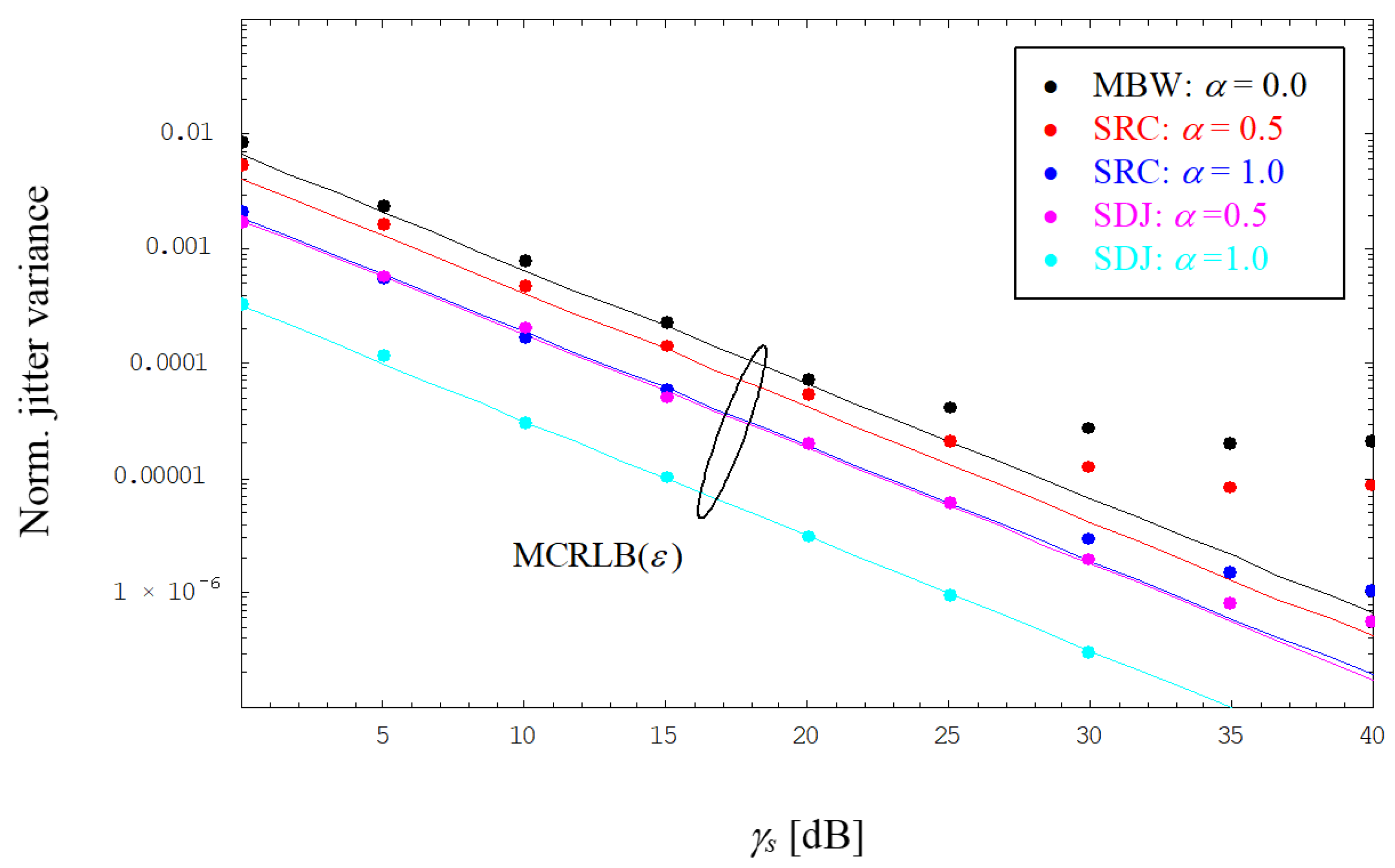
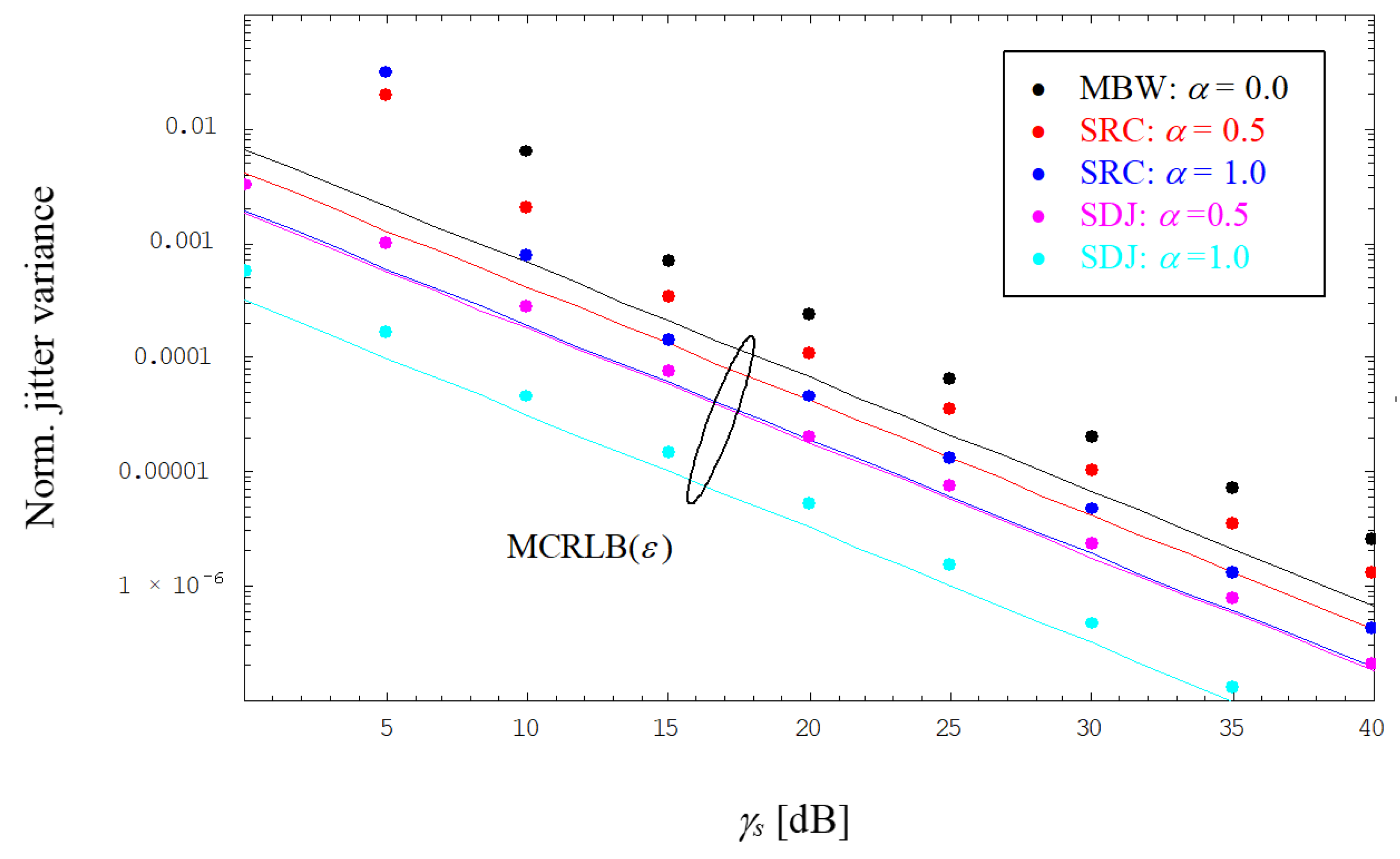
As a function of the electrical SNR value defined in (6), Figure 5 and Figure 6 depict the evolution of the normalized jitter variance for timing estimates using an MF or FF receiver, respectively, and operating the link with SRC or SDJ shapes. By detailed inspection of Figure 5, we observe that the MF solution is close to the MCRLB in the medium-to-low SNR range, whereas for larger SNRs, the jitter performance ends up in an error floor, which is obviously less severe for higher values of α. This phenomenon is explained by the fact that the receiver MF violates the Nyquist property of the SRC/SDJ shape, producing this way an ISI effect that does not disappear, even if the AWGN component vanishes when γ_s → ∞. In addition, it is to be noticed that SDJ pulses exhibit a better jitter performance than do SRC shapes; note that for α = 0, both scenarios converge to the MBW case.

For comparison purposes, the FF results are shown in Figure 6. We can see immediately that the FF variant exhibits no floor effect, simply because the receiver filter does not distort the orthogonality of the SRC/SDJ function. On the other hand, it is to be noticed that the jitter performance is only close to the MCRLB for higher values of α and γ_s > 10 dB; otherwise, the performance degrades compared to MF, mainly because significantly more noise passes the flat filter.

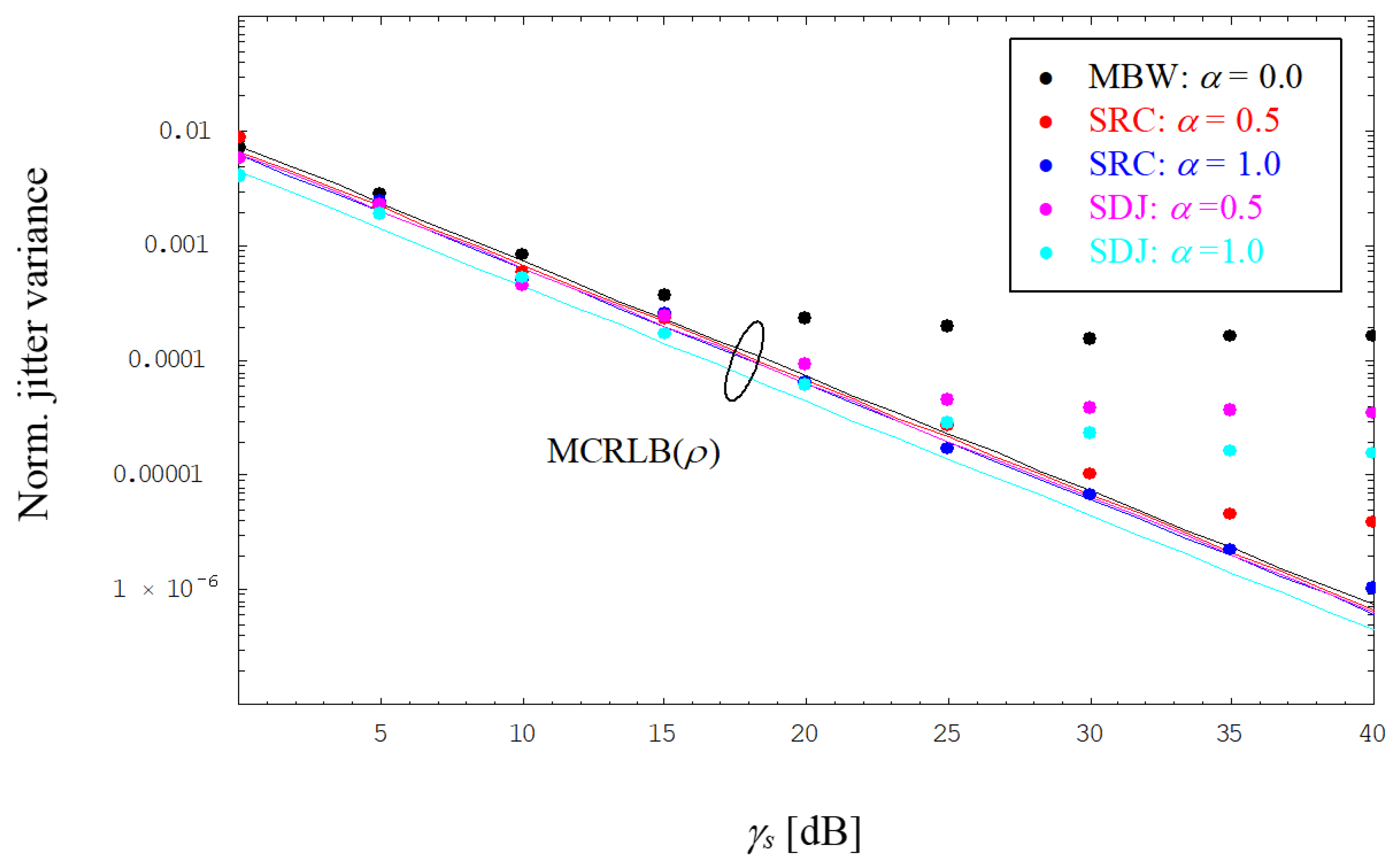
Additionally, as a function of the average electrical SNR, Figure 7 and Figure 8 show the evolution of the normalized jitter variance of amplitude estimates using MF and FF scenarios, respectively, again operating the link with SRC or SDJ shapes. In contrast to the recovery of the symbol timing, the MCRLB is more or less the same, irrespective of the chosen excess bandwidth. This is also confirmed in Figure 7 by numerical results achieved in the lower SNR range, where they are close to the MCRLB. For larger SNRs, we observe an error floor caused by the violation of the Nyquist condition; again, this sort of degradation is less severe for increasing values of α. Interestingly, given the same roll-off factor, the floor effect is more pronounced for SDJ than for SRC.

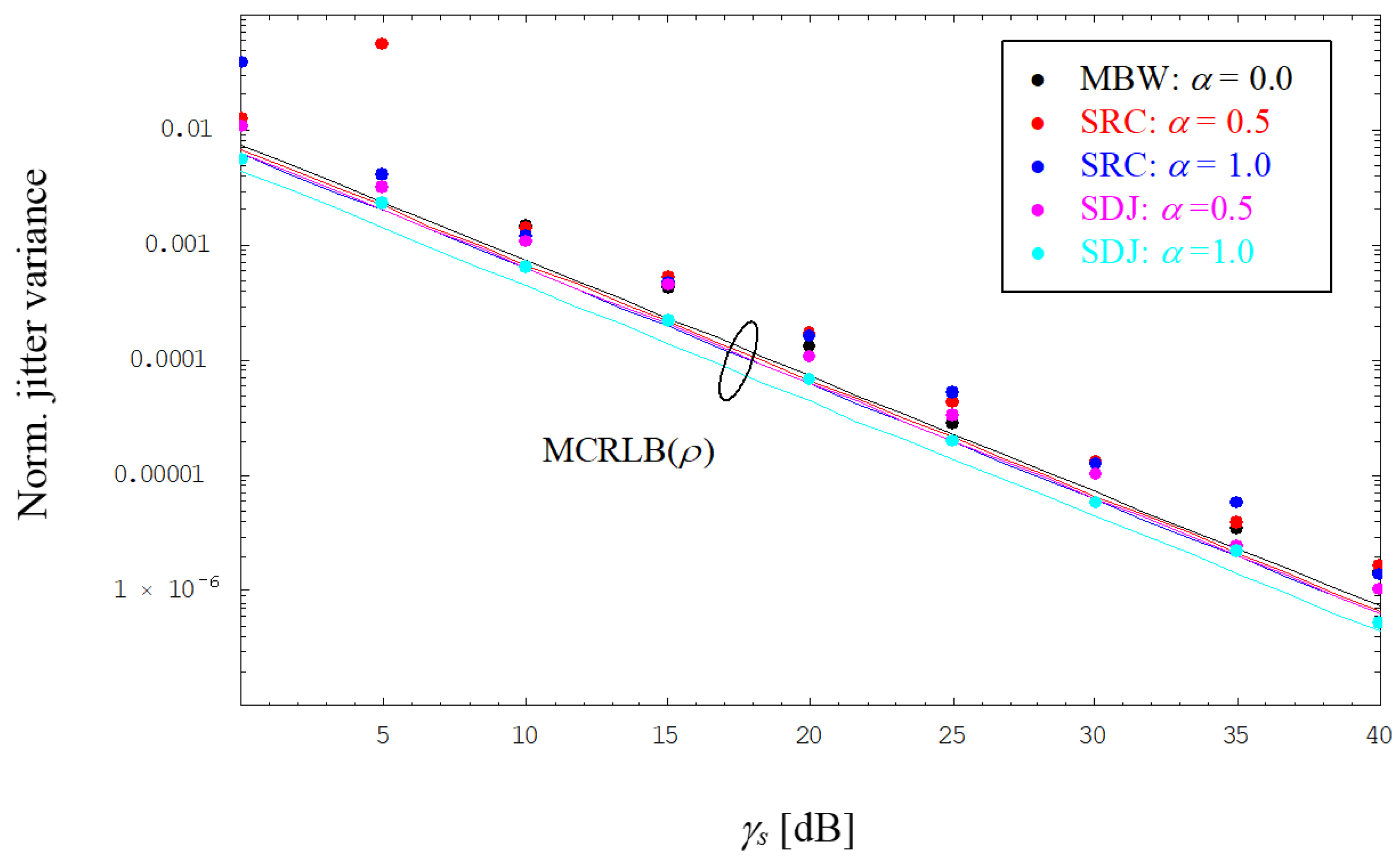
Not surprisingly, the jitter floor vanishes by application of the FF method, whose jitter performance is visualized in Figure 8. Due to the larger amount of noise at the FF output, we face a higher jitter variance compared to results in Figure 7 by taking the MCRLB as a benchmark; solely for smaller values of SNR and α, the error performance worsens somewhat due to an increasing number of outliers caused by a failure of the estimator algorithm.

6. Conclusions

Assuming a pulse shaping embodied by SRC and SDJ functions, the estimation of symbol timing and signal amplitude has been studied in the context of a bandlimited optical intensity link. To this end, the modified Cramer–Rao lower bound was derived as the theoretical limit of the jitter variance exhibited by an estimator algorithm. Regarding the latter, it turned out that a maximum likelihood solution is suboptimal, because it involves a receiver matched filter violating the Nyquist criterion such that the jitter performance ends up in an error floor. It could be verified that this drawback might be circumvented by a flat filter structure, although the jitter variance increases somewhat in this case, because of a larger amount of noise passing the filter.

A subject for future research is the extension of the estimation problem to a non-data-aided situation [21], i.e., data symbols need not be known to the receiver in the form of preambles or pilot sequences, increasing in this way the spectral efficiency of the optical link.

References

- Hranilovic, S. Wireless Optical Communication Systems; Springer: New York, NY, USA, 2004. [Google Scholar]
- Arnon, S.; Barry, J.; Karagiannidis, G.; Schober, R.; Uysal, M. Advanced Optical Wireless Communication Systems; Cambridge Univ. Press: New York, NY, USA, 2012. [Google Scholar]
- Khalighi, M.-A.; Uysal, M. Survey on Free Space Optical Communication: A Communication Theory Perspective. IEEE Commun. Surveys Tutorials 2014, 16, 2231–2258. [Google Scholar] [CrossRef]
- Ghassemlooy, Z.; Arnon, S.; Uysal, M.; Xu, Z.; Cheng, J. Emerging Optical Wireless Communications—Advances and Challenges. IEEE J. Select. Areas Commun. 2015, 33, 1738–1749. [Google Scholar] [CrossRef]
- Wang, J.-Y.; Liu, C.; Wang, J.-B.; Wu, Y.; Lin, M.; Cheng, J. Physical-layer security for indoor visible light communications: Secrecy capacity analysis. IEEE Trans. Commun. 2018, 66, 6423–6436. [Google Scholar] [CrossRef]
- Hranilovic, S. Minimum-bandwidth optical intensity Nyquist pulses. IEEE Trans. Commun. 2007, 55, 574–583. [Google Scholar] [CrossRef]
- Tavan, M.; Agrell, E.; Karout, J. Bandlimited intensity modulation. IEEE Trans. Commun. 2012, 60, 3429–3439. [Google Scholar] [CrossRef]
- Czegledi, C.; Khanzadi, M.R.; Agrell, E. Bandlimited power-efficient signaling and pulse design for intensity modulation. IEEE Trans. Commun. 2014, 62, 3274–3284. [Google Scholar] [CrossRef]
- Karout, J.; Kramer, G.; Kschischang, F.R.; Agrell, E. A two-dimensional signal space for intensity-modulated channels. IEEE Commun. Lett. 2012, 16, 1361–1364. [Google Scholar] [CrossRef]
- Zhang, D.; Hranilovic, S. Bandlimited optical intensity modulation under average and peak power constraints. IEEE Trans. Commun. 2016, 64, 3820–3830. [Google Scholar] [CrossRef]
- Mengali, U.; D’Andrea, A.N. Synchronization Techniques for Digital Receivers; Plenum Press: New York, NY, USA, 1997. [Google Scholar]
- Meyr, H.; Moeneclaey, M.; Fechtel, S.A. Digital Communication Receivers: Synchronization, Channel Estimation, and Signal Processing; Wiley: New York, NY, USA, 1998. [Google Scholar]
- Kay, S.M. Fundamentals of Statistical Signal Processing: Estimation Theory; Prentice Hall: Upper Saddle River, NJ, USA, 1993. [Google Scholar]
- Wang, J.-B.; Xie, X.-X.; Jiao, Y.; Chen, M. Training sequence based frequency-domain channel estimation for indoor diffuse wireless optical communications. EURASIP J. Wireless Commun. Network. 2012, 326, 1–10. [Google Scholar] [CrossRef]
- D’Andrea, A.N.; Mengali, U.; Reggiannini, R. The modified Cramer-Rao bound and its application to synchronization problems. IEEE Trans. Commun. 1994, 42, 1391–1399. [Google Scholar] [CrossRef]
- Gini, F.; Reggiannini, R.; Mengali, U. The modified Cramer-Rao bound in vector parameter estimation. IEEE Trans. Commun. 1998, 46, 52–60. [Google Scholar] [CrossRef]
- Moeneclaey, M. On the true and the modified Cramer-Rao bounds for the estimation of a scalar parameter in the presence of nuisance parameters. IEEE Trans. Commun. 1998, 46, 1536–1544. [Google Scholar] [CrossRef]
- Gappmair, W.; Ginesi, A. Cramer-Rao lower bound and parameter estimation for multibeam satellite links. Int. J. Satellite Commun. Network. 2017, 35, 343–357. [Google Scholar] [CrossRef]
- Press, W.H.; Teukolsky, S.A.; Vetterling, W.T.; Flannery, B.P. Numerical Recipes in C: The Art of Scientific Computing; Cambridge Univ. Press: New York, NY, USA, 1992. [Google Scholar]
- Suesser-Rechberger, B.; Gappmair, W. New results on symbol rate estimation in digital satellite receivers. In Proceedings of the 11th IEEE/IET Int. Symp. Commun. Systems, Networks and Digital Signal Processing, Budapest, Hungary, 18–20 July 2018; pp. 1–6. [Google Scholar]
- Tabiri, M.T.; Sadough, S.M.S.; Khalighi, M.-A. FSO communication for high speed trains: Blind data detection and channel estimation. In Proceedings of the 11th IEEE/IET Int. Symp. Commun. Systems, Networks and Digital Signal Processing, Budapest, Hungary, 18–20 July 2018; pp. 1–4. [Google Scholar]
Figure 1.
Evolution of different pulse shapes. MBW is minimum bandwidth, SRC is squared raised cosine, SDJ is squared double jump.
Figure 2.
Signal model for intensity modulation and direct detection (IM/DD) optical links.
Figure 3.
Mean estimator value (MEV) for timing recovery using SRC shapes (matched filter (MF) receiver).
Figure 4.
Mean estimator value for amplitude recovery using SDJ shapes (flat filter (FF) receiver).
Figure 5.
Normalized jitter variance for timing estimates (MF receiver). MCRLB is the modified Cramer-Rao lower bound.
Figure 6.
Normalized jitter variance for timing estimates (FF receiver).
Figure 7.
Normalized jitter variance for amplitude estimates (MF receiver).
Figure 8.
Normalized jitter variance for amplitude estimates (FF receiver).
© 2019 by the author. Licensee MDPI, Basel, Switzerland. This article is an open access article distributed under the terms and conditions of the Creative Commons Attribution (CC BY) license (http://creativecommons.org/licenses/by/4.0/).
Share and Cite
MDPI and ACS Style
Gappmair, W. On Parameter Estimation for Bandlimited Optical Intensity Channels. Computation 2019, 7, 11. https://0-doi-org.brum.beds.ac.uk/10.3390/computation7010011
AMA Style
Gappmair W. On Parameter Estimation for Bandlimited Optical Intensity Channels. Computation. 2019; 7(1):11. https://0-doi-org.brum.beds.ac.uk/10.3390/computation7010011
Chicago/Turabian StyleGappmair, Wilfried. 2019. "On Parameter Estimation for Bandlimited Optical Intensity Channels" Computation 7, no. 1: 11. https://0-doi-org.brum.beds.ac.uk/10.3390/computation7010011
Note that from the first issue of 2016, this journal uses article numbers instead of page numbers. See further details here.