Multi Similarity Metric Fusion in Graph-Based Semi-Supervised Learning

Abstract

In semi-supervised label propagation (LP), the data manifold is approximated by a graph, which is considered as a similarity metric. Graph estimation is a crucial task, as it affects the further processes applied on the graph (e.g., LP, classification). As our knowledge of data is limited, a single approximation cannot easily find the appropriate graph, so in line with this, multiple graphs are constructed. Recently, multi-metric fusion techniques have been used to construct more accurate graphs which better represent the data manifold and, hence, improve the performance of LP. However, most of these algorithms disregard use of the information of label space in the LP process. In this article, we propose a new multi-metric graph-fusion method, based on the Flexible Manifold Embedding algorithm. Our proposed method represents a unified framework that merges two phases: graph fusion and LP. Based on one available view, different simple graphs were efficiently generated and used as input to our proposed fusion approach. Moreover, our method incorporated the label space information as a new form of graph, namely the Correlation Graph, with other similarity graphs. Furthermore, it updated the correlation graph to find a better representation of the data manifold. Our experimental results on four face datasets in face recognition demonstrated the superiority of the proposed method compared to other state-of-the-art algorithms.

1. Introduction

In machine learning problems, representing the manifold of the data is a key point, and it is a cornerstone in many semi-supervised learning methods. One of the most useful tools for representing an intrinsic structure of the data is the use of a graph [1]. In addition, the graph can encode pairwise similarities between the samples. Since the goal is to find an appropriate similarity metric for the data space, it is hard to define a fixed and single similarity metric. Multi-metric fusion refers to a type of fusion that combines different metrics [2,3,4,5]. Using different similarity metrics and considering their connection can improve and robustify the performance of learning tasks [2,4,5].

In semi-supervised learning, graphs can be used in many tasks, such as classification [6,7], clustering [8,9,10], dimension reduction [11,12], and label propagation (LP) [13,14], to mention a few. In a semi-supervised learning context, very often data comprise two subsets of labeled and unlabeled samples. One main task of semi-supervised learning is graph-based LP. This aims to propagate the label of labeled data to unlabeled ones over the graph [15]. LP has different applications in community detection [16], image segmentation [17], clustering [18], and classification [19] tasks. Although most of the algorithms use one single graph as an input of the LP algorithms, such as the Zhou method [20], flexible manifold embedding (FME) [21], local and global consistency (LGC) [22], and Gaussian fields and harmonic function (GFHF) [23], exploiting various similarity graphs can enhance the performance of LP process (graph-fusion methods) [15,24,25,26,27,28], thereby creating multiple similarity graphs where each contains complementary information of data and fusing them together can lead to a better representation of data.

The manifestation of the Internet and technology caused the growth of data in multiple forms as video, image, audio, text, etc. [29,30]. The key is how to integrate them to benefit complementary information from each view. Therefore, graph fusion methods have been proposed as one of the approaches to fuse different views. While different algorithms for graph fusion have been designed in three levels of graph integration (early integration [31], late integration [15], and intermediate integration [24,25,26,27,28,32,33]), a common solution is to construct different graphs based on multiple views called intermediate integration and then fuse the graphs either linearly via dynamic graph fusion LP (DGFLP) [25], sparse multiple graph integration (SMGI) [24], multi-view LGC [32], and deep graph fusion [33]), or nonlinearly with similarity network fusion (SNF) [27], nonlinear graph fusion (NGF) [26], and multi-modality dynamic LP (MDLP) for semi-supervised multi-class multi-label [28]. Furthermore, some methods attempt to learn different metrics based on different feature descriptors [2,3,4,5], whereas, in some cases, the variation of multi-view leads to misalignment in feature descriptors [34]. So, determining the discriminant and reliable feature descriptor is a key point [35]. To solve this problem, some algorithms build different types of similarity graphs based on an available view [24] and merge them to be used in the LP process.

Constructing an appropriate single similarity graph that represents the exact manifold of data is not a trivial task. Some research provides different similarity graphs by adopting different parameters in the graph construction scheme. Moreover, this approach depends on the parameters of the similarity graph and the way they are adjusted.

The data space, which is known as the feature space is the main source of information about the data samples. Although, label space has some information that can be integrated with the data space, which makes the graph construction more robust to noises and outliers [31], very few works have used this information in the fusion process [25,28,31]. The joint use of the label space and feature space can boost the performance of LP [25,28,31].

The contributions of this paper are as follows: We proposed a new multi-metric algorithm that integrates graph fusion and LP in a unified framework. With respect to this, we extended the FME LP method to fuse multiple similarity graphs based on a single feature descriptor of data. Since the relevance of all graphs was equal, the proposed method did not seek to weigh the individual metrics. In addition, to further improve the performance, we integrated the information in the label space with the feature space. Exploiting the label space was achieved by constructing a graph based on the correlation between the label vectors (both available and predicted ones).

The rest of the paper is outlined as the follows: Section 2 briefly explains multi-metric method, and Section 3 describes the proposed method in detail. Our experimental results are reported in Section 4, and Section 5 provides the discussion and conclusion.

2. An Overview on Multi-Metric Fusion

A metric or distance function refers to a function that explains a distance between pair-wise samples. A similarity metric defines a similarity function that measures how two samples are similar or related. Depending on the adopted feature descriptor, a metric can well discriminate between the samples, however, finding an individual proper metric is difficult. Multi-metric methods proposed exploiting different metrics corresponding to different views of data [5]. Moreover, even a simple metric like k-Nearest Neighbors (k-NN) graph has parameters (e.g., number of neighbors) to tune where correct tuning of the parameters can have an important effect on the results.

Recently proposed methods in semi-supervised learning fused several graphs in order to maximize inter-class scattering and minimize the variation of intra-class [36]. This strategy also achieves the complementary information from each view and enhances the performance of the classification [24,25,28].

In Reference [24], the authors proposed an SMGI algorithm that integrates a set of k-NN graphs with different values of K (neighborhood parameter) linearly with some noisy graphs. This method is adopted for a semi-supervised learning task. They assigned unequal weight to each graph and sparsely selected the relevant graphs from the noisy ones. They only used one type of similarity graph with different parameters and do not employ label space in its fusion approach.

In Reference [28], the authors proposed an MDLP algorithm which utilized multiple views (each sample has multiple descriptors) in semi-supervised learning. A feature descriptor was associated with each view. Two types of k-NN graphs were then constructed from each descriptor. A local k-NN graph which considered the similarity of each sample to its local neighbors and the global k-NN graph focused on the similarity of each sample to all other samples. In the fusion process, the information of label space integrated with these two graphs.

In Reference [25] the authors proposed a DGFLP method that fused the information of data and label spaces together. The algorithm allocates dynamic unequal weights to each constructed graph, while uses a fixed weight for the information of the label space.

Another semi-supervised multi-graph fusion is presented in [32]. It extended the LGC [22] method to the multi-view case (MLGC). They constructed one graph for each adopted feature descriptor and then combined them linearly with equal weights. This approach used only one type of similarity metric and, furthermore, it ignored employing label space information in its fusion process.

In our previous work [33], we concentrated on the multi-view fusion scenario, where the goal was to merge different available information of data samples. A graph was constructed based on each feature and then they were merged by summing them linearly to obtain the final graph.

3. Proposed Method

Consider that we have a dataset X = [x₁, x₂, …, x_N] that contains N samples whose dimension is equal to d. Suppose we have C classes index by c = 1, 2, …, C, then Y ∈ R^N×C is the initial binary label matrix, where y(i,c) represents the probability value of sample ith belonging to the class c. In semi-supervised learning, few data samples have labels, but the majority of them have no labels. The objective is to predict the labels of unlabeled data via a graph which propagates the labels of labeled data to their nearby unlabeled data. The output of LP is the prediction label matrix (F).

A graph is a data structure with three components G = (V,E,W). V denotes the nodes of the graph, E represents the edges on the graph, and W ∈ R^N×N is the similarity matrix. The similarity value between the two nodes i and j, is given by the entry w(i,j) of the similarity matrix. Since we do not have precise prior knowledge about the appropriate similarity graph, we choose a strategy that combines several different graphs.

As an example, consider the k-NN graph construction technique, a graph construction method that makes an edge and connects each sample to its K nearest neighbors. The weight of each edge can be computed by different algorithms and the most common one is called the Gaussian kernel [15,37,38] function as:

$${\mathrm{w}}_{\mathrm{i}\mathrm{j}}=\exp (\frac{{-\Vert {\mathbf{x}}_{\mathrm{i}}-{\mathbf{x}}_{\mathrm{j}}\Vert }^2}{{2\mathsf{\sigma }}^2})$$

(1)

where, x_i and x_j represents the node i and j, respectively, and σ is the width of the Gaussian kernel. The value of σ can be defined either manually or adaptively [39]. The rows of the affinity matrix are then normalized to have sum equals to one adopting the Equation (2). Finally, the matrix is made symmetric using Equation (3).

$${\mathrm{w}}_{\mathrm{i}\mathrm{j}}=\frac{{\mathrm{w}}_{\mathrm{i}\mathrm{j}}}{{{\displaystyle \sum }}_{\mathrm{j}=1}^{\mathrm{N}}{\mathrm{w}}_{\mathrm{i}\mathrm{j}}}$$

(2)

$$\mathbf{W}=\frac{1}{2}(\mathbf{W}+{\mathbf{W}}^{\mathrm{T}})$$

(3)

Let L denote the graph Laplacian matrix, which is obtained by L = D − W. D is a degree matrix, where $\mathbf{D}(\mathrm{i},\mathrm{i})={{\displaystyle \sum }}_{\mathrm{j}=1}^{\mathrm{N}}\mathrm{w}(\mathrm{i},\mathrm{j})$ represents its diagonal elements.

Table 1. List of mathematical notations.

Notation	Description
N	Number of samples
M	Number of metrics
X = [x1, x2, …, xN]	Data matrix
C	Number of classes
d	Sample dimension
Y	Initial binary label matrix
F	Prediction label matrix
W	Similarity matrix
L	Laplacian matrix
$\widehat{L}$	Fusion Laplacian matrix
Q	Projection matrix
b	Bias vector
t	Iteration number

shows all the notations that were used in the paper.

3.1. Review of Flexible Manifold Embedding (FME)

FME [21] is an LP framework that was proposed in 2010. This method can be used in both semi-supervised and unsupervised learning settings. The objective function of FME is given by:

$${\mathrm{argmin}}_{\mathbf{F},\mathbf{Q},\mathrm{b}}\left\{\mathrm{Trace}\left({\mathbf{F}}^{\mathrm{T}}\mathbf{L}\mathbf{F}\right)+\mathrm{Trace}{\left(\mathbf{F}-\mathbf{Y}\right)}^{\mathrm{T}}\mathbf{U}\left(\mathbf{F}-\mathbf{Y}\right)+\mathsf{\mu }\left({{\Vert \mathbf{Q}\Vert }^2+\mathsf{\gamma }\Vert {\mathbf{X}}^{\mathrm{T}}\mathbf{Q}+\mathbf{1}{\mathbf{b}}^{\mathrm{T}}-\mathbf{F}\Vert }^2\right)\right\},$$

(4)

where L, F, and Y are the Laplacian matrix, the prediction label matrix, and the initial label matrix, respectively. U is the diagonal matrix such that the diagonal elements for labeled nodes are 1 and for unlabeled nodes are 0. In unsupervised learning, as there is no predefined label, the second term is eliminated by setting all elements of U to 0. μ and γ are the trade-off parameters. X is the training data matrix, Q is the projection matrix that maps feature space to label space, b is the bias vector, and 1 is a vector that each element of it is one. The projection matrix Q ∈ R^d×C and the bias vector b ∈ R^C×1 are used for estimating the labels of unseen data.

In Equation (4), the first term of the cost function represents the smoothness assumption and the second term is the prediction error for the labeled data. The last term is the error of the projection from the data space into the label space. The outputs of the algorithm are the prediction label matrix (F), the projection matrix (Q), and the bias vector (b). This method uses a projection matrix to map data space to label space through a linear regression function. Optimal F, Q, and b can be obtained using the closed-form solution as (see Reference [21] for more details):

$$\begin{array}{c}\mathbf{F}={(\mathbf{U}+\mathbf{L}+\mathsf{\mu }\mathsf{\gamma }{(\mathbf{B}-\mathbf{I})}^{\mathrm{T}}(\mathbf{B}-\mathbf{I})+\mathsf{\mu }{\mathbf{A}}^{\mathrm{T}}\mathbf{A})}^{-1}\mathbf{U}\mathbf{Y}\\ \mathbf{B}={\mathbf{H}}_{\mathrm{c}}{\mathbf{X}}^{\mathrm{T}}\mathbf{A}+(\frac{1}{\mathrm{n}}){\mathbf{11}}^{\mathrm{T}}\\ {\mathbf{H}}_{\mathrm{c}}=\mathbf{I}-(\frac{1}{\mathrm{n}}){\mathbf{11}}^{\mathrm{T}}\\ \mathbf{A}=\mathsf{\gamma }{(\mathsf{\gamma }\mathbf{X}{\mathbf{H}}_{\mathrm{c}}{\mathbf{X}}^{\mathrm{T}}+\mathbf{I})}^{-1}\mathbf{X}{\mathbf{H}}_{\mathrm{c}}\end{array}$$

(5)

$$\mathbf{Q}=\mathbf{A}\mathbf{F}$$

(6)

$$\mathbf{b}=\frac{1}{\mathrm{n}}({\mathbf{F}}^{\mathrm{T}}\mathbf{1}-{\mathbf{W}}^{\mathrm{T}}\mathbf{X}\mathbf{1}),$$

(7)

where n is the total number of samples.

Regarding this method, we extended it to multi-metric fusion algorithm, which integrates multiple graphs and incorporates the label space into the fusion process.

3.2. Multi Similarity Metric Fusion

According to our available view, we build M different similarity graphs (denoted as W_i for the ith metric) based on M different metrics. Corresponding to each graph, we have a Laplacian matrix (i.e., L_i). With respect to [15,28], we suppose that the manifold structure of data is attained by a linear integration of multiple graphs as ${{\displaystyle \sum }}_{\mathrm{i}=1}^{\mathrm{M}}{\mathbf{W}}_{\mathrm{i}}$. Similar to this idea in our proposed method, we extended the smooth manifold term of FME as:

$${{\displaystyle \sum }}_{\mathrm{i}=1}^{\mathrm{M}}\mathrm{Trace}({\mathbf{F}}^{\mathrm{T}}{\mathbf{L}}_{\mathrm{i}}\mathbf{F}).$$

(8)

If we consider ${\mathbf{L}}_{\mathrm{data}}={{\displaystyle \sum }}_{\mathrm{i}=1}^{\mathrm{M}}{\mathbf{L}}_{\mathrm{i}}$, then we have:

$$\mathrm{Trace}({\mathbf{F}}^{\mathrm{T}}({{\displaystyle \sum }}_{\mathrm{i}=1}^{\mathrm{M}}{\mathbf{L}}_{\mathrm{i}})\mathbf{F}):=\mathrm{Trace}({\mathbf{F}}^{\mathrm{T}}{\mathbf{L}}_{\mathrm{data}}\mathbf{F}),$$

(9)

where, L_data is the Laplacian fusion of the graphs constructed based on different metrics. By replacing this equation in the first term of the FME algorithm, our cost function is obtained as:

$${\mathrm{argmin}}_{\mathrm{F},\mathrm{Q},\mathrm{b}}\left\{\mathrm{Trace}\left({\mathbf{F}}^{\mathrm{T}}{\mathbf{L}}_{\mathrm{data}}\mathbf{F}\right)+\mathrm{Trace}{\left(\mathbf{F}-\mathbf{Y}\right)}^{\mathrm{T}}\mathbf{U}\left(\mathbf{F}-\mathbf{Y}\right)+\mathsf{\mu }\left({\Vert \mathbf{Q}\Vert }^2+\mathsf{\gamma }{\Vert {\mathbf{X}}^{\mathrm{T}}\mathbf{Q}+\mathbf{1}{\mathrm{b}}^{\mathrm{T}}-\mathbf{F}\Vert }^2\right)\right\},$$

(10)

where the first term fuses M metrics from an available feature descriptor. The last two terms are the same as the last two terms in the FME algorithm.

3.3. Incorporating Label Space Information

A feature descriptor, which is known as the data space, extracts information of data. The works of Reference [25,28,31] demonstrate that there is some hidden information in the label space which is ignored. As the similarity of two vectors can be described by the correlation of them, so by calculating the correlation of predicted labels, we can define a new similarity measure in the label space. The concept of it is that if two samples have a slight similarity in the data space, it is possible that they have a strong similarity in the label space. Here, the label space can affect the similarity between them.

The main key is how to merge the label space with the data space. We proposed a new similarity metric based on label space. In fact, we considered the label space as a new view of the data that could be described by a new similarity metric. The nodes of the graph were the samples and the weight of each edge was computed by the Pearson correlation measure, as shown in Equation (11). For two samples, x_i and x_j with the label vectors f_i and f_j, the similarity between them was calculated as:

$$\mathrm{correlation}({\mathrm{f}}_{\mathrm{i}},{\mathrm{f}}_{\mathrm{j}}):=\frac{{{\displaystyle \sum }}_{\mathrm{q}=1}^{\mathrm{c}}({\mathrm{f}}_{\mathrm{q}\mathrm{i}}-{\overline{\mathrm{f}}}_{\mathrm{i}})({\mathrm{f}}_{\mathrm{q}\mathrm{j}}-{\overline{\mathrm{f}}}_{\mathrm{j}})}{\sqrt{{{\displaystyle \sum }}_{\mathrm{q}=1}^{\mathrm{c}}{({\mathrm{f}}_{\mathrm{q}\mathrm{i}}-{\overline{\mathrm{f}}}_{\mathrm{i}})}^2}\sqrt{{{\displaystyle \sum }}_{\mathrm{q}=1}^{\mathrm{c}}{({\mathrm{f}}_{\mathrm{q}\mathrm{j}}-{\overline{\mathrm{f}}}_{\mathrm{j}})}^2}},$$

(11)

where, ${\overline{\mathrm{f}}}_{\mathrm{i}}$ and ${\overline{\mathrm{f}}}_{\mathrm{j}}$ were the average of vectors f_i and f_j.

Afterward, we omitted negative values obtained by correlation measure and for each sample, the K highest similar samples were chosen as its K neighbors. We called this new similarity metric the correlation graph. To incorporate the label space graph with the data space graph, we linearly added it to the graphs obtained by other metrics with equal weights as:

$$\widehat{\mathbf{L}}:={\mathbf{L}}_{\mathrm{data}}+{\mathbf{L}}_{\mathrm{Corr}},$$

(12)

where L_Corr is the Laplacian of the correlation graph. Since the predicted labels changed in each iteration, the correlation graph changed, too. After each iteration of LP, the obtained $\widehat{\mathbf{L}}$ would be used (instead of L_data) in the cost function of the proposed multi-view FME of Equation (10).

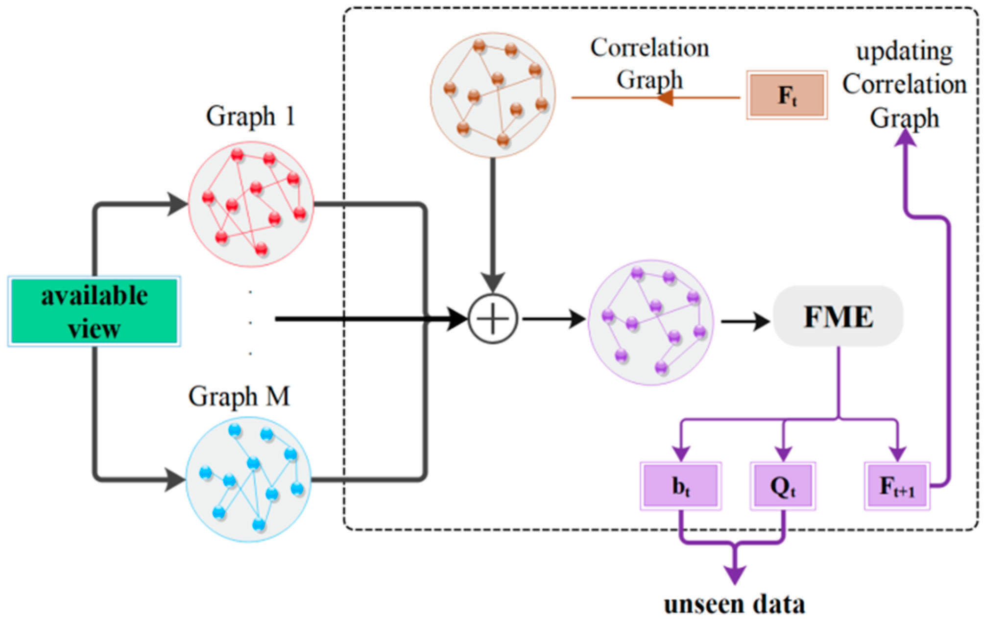
The framework of our proposed method is depicted in Figure 1. From the available views, M graphs were constructed. Also, a correlation graph was created based on the initial label matrix Y. Then, all the graphs became integrated by a linear fusion with equal weights and were fed to FME LP method. The FME algorithm estimated the label matrix F, Q projection matrix, and the b bias vector. In the next iteration of fusion, the correlation graph updated based on the correlation of predicted matrix F. This process was repeated through a given number of iterations. In the last iteration, the projection matrix and the bias vector could be used for estimating the labels of unseen data, which were not available at first.

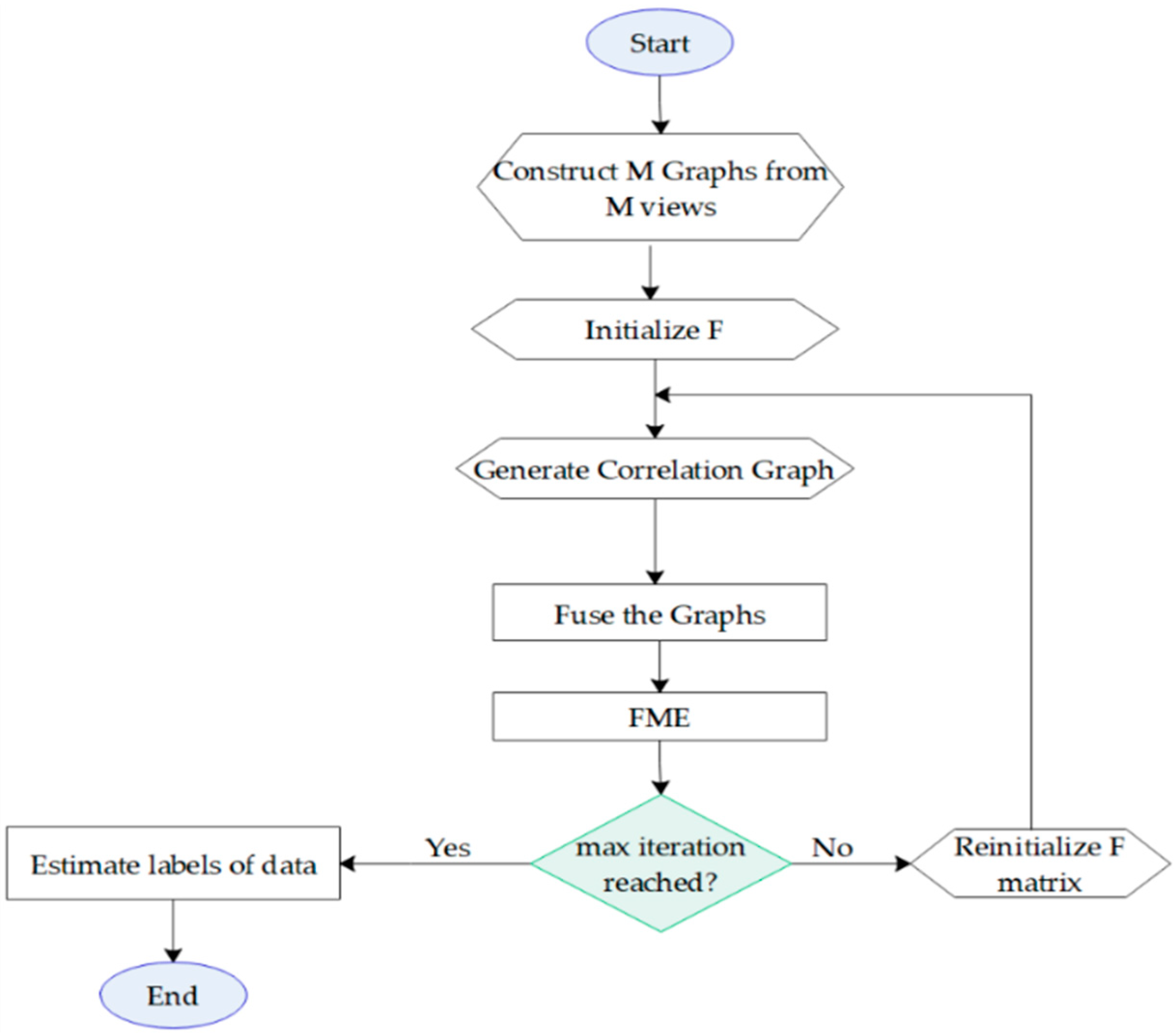
We summarize the procedure of our proposed method in Algorithm 1. Moreover, Figure 2 shows the flowchart of the proposed method.

Algorithm 1. The proposed method.

Input: Feature from one view X;

Initial label matrix Y = [Y1, Yu];

Parameters μ and γ.

Output: Predicted label matrix F, projection matrix Q, and bias vector b.

1. Construct M different graphs from the available view.

2. Compute the Laplacian matrices of the graphs.

3. Initialize the soft label matrix F = Y.

4. for t = 1: Max iteration.

5. Generate the correlation graph based on F by Equation (11).

6. Fuse the M + 1 Laplacian graph to obtain $\widehat{\mathbf{L}}$ adopting Equation (12).

7. Feed $\widehat{\mathbf{L}}$ to FME and calculate a new soft label matrix F.

8. Reinitialize the part of F matrix corresponding to the labeled samples.

9. end for.

10. To calculate the labels of unseen samples, use the projection matrix Q and the bias vector b to predict the labels of them.

4. Experimental Results

4.1. Experimental Setup

We evaluated the proposed method using four real-world face datasets, PF01 [40], Extended Yale (http://vision.ucsd.edu/~leekc/ExtYaleDatabase/ExtYaleB.html), PIE (http://www.ri.cmu.edu/projects/project_418.html), and the subsets of FERET [41], and compared the performance results with other recently proposed graph fusion methods. The details of each dataset are reported in

Table 2. Statistics of datasets used in experiments.

Dataset	Size	# of Classes	Features	Dimension
PF01	1819	107	VGG Face-FC7	4096
			VGG Face-FC6	4096
			LBP	900
Extended_Yale	1774	28	VGG Face-FC7	4096
			VGG Face-FC6	4096
			LBP	900
PIE	1926	68	VGG Face-FC7	4096
			VGG Face-FC6	4096
			LBP	900
FERET	1400	200	VGG Face-FC7	4096
			VGG Face-FC6	4096
			LBP	900

. The experiments were conducted on a PC equipped with an i5-4300U 1.9 GHz 2.5 GHz CPU and 8 GB of RAM.

We extracted three features from the face images. Two Deep features are extracted from the pre-trained VGG Face model [42] and Local Binary Pattern (LBP) image [43] was the handcrafted feature. For deep features, we used two fully-connected layers of VGG Face model, namely FC6 and FC7. For the handcrafted feature, we applied LBP on the image, and the output was reshaped to form a single vector.

In the graph construction step, we adopted two graphs, the K-nearest neighbor graph and the adaptive k-NN graph, both with the Gaussian kernel to weight the edges. To keep the k-NN graphs as sparse as possible, we set the number of neighbors K = 3. For the k-NN graph, the sigma of the Gaussian kernel was empirically set to σ = 0.05, and for the adaptive one, it would be selected automatically, according to:

$$\mathsf{\sigma }=\frac{1}{\mathrm{N}}{\displaystyle \sum }_{\mathrm{i}=1}^{\mathrm{N}}\mathrm{dis}({\mathbf{x}}_{\mathrm{i}},{\mathbf{x}}_{\mathrm{i}\mathrm{K}})$$

(13)

where ${\mathbf{x}}_{\mathrm{i}\mathrm{K}}$ is the Kth closest node to sample x_i, and dis(x_i, x_j) is the Euclidian distance between nodes x_i and x_j. For FME parameters, we selected μ = 10³ and γ = 10⁻³. Since our method was an iterative process, we empirically set Algorithm 1’s number of iterations to 10. We stress the fact that we did not optimize any of the aforementioned parameters because their optimum values depended on the datasets.

In Section 4.2, we assessed the effect of using multiple similarity graphs into the FME framework, and in Section 4.3, we compared the proposed method with other state-of-art graph fusion algorithms. In Section 4.4, we demonstrated the CPU-time of our proposed method with other methods.

4.2. Comparison with Individual Graphs

In this section, the performance of our multi-metric fusion method was compared with that of individual graphs using the same FME method. The average accuracy over 10 random combinations of labeled and unlabeled data was reported in

Table 3. Mean accuracy and standard deviation of label propagation (LP) for the individual feature and the proposed method. K-NN = k-Nearest Neighbor.

Dataset	# Labeled Samples	Feature	Accuracy (Mean ± STD )
			k-NN graph	Adaptive k-NN Graph	Proposed Method
PF01	1	FC7	89.63 ± 7.97	89.07 ± 8.39	92.42 ± 2.86
		FC6	90.85 ± 7.16	89.54 ± 8.99	93.99 ± 0.85
		LBP	51.79 ± 11.64	49.16 ± 11.54	56.19 ± 8.97
	2	FC7	94.16 ± 1.09	93.94 ± 1	94.36 ± 1.19
		FC6	94.74 ± 1.04	94.22 ± 1.11	94.75 ± 0.98
		LBP	63.77 ± 6.82	61.08 ± 6.98	65.47 ± 5.86
Extended_Yale	1	FC7	40.33 ± 20.86	40.33 ± 20.94	43.5 ± 19.34
		FC6	44.67 ± 22.76	44.32 ± 22.9	50.38 ± 19.27
		LBP	91.32 ± 5.17	91.69 ± 5.66	94.25 ± 1.52
	2	FC7	54.24 ± 22	54.13 ± 21.99	55.35 ± 21.68
		FC6	57.01 ± 22.99	56.81 ± 23.06	58.68 ± 21.77
		LBP	96.01 ± 2.3	96.17 ± 2.07	96.73 ± 1.93
PIE	1	FC7	77.36 ± 9.82	77.17 ± 9.79	79.04 ± 8.21
		FC6	76.52 ± 11.43	75.73 ± 11.7	79.77 ± 8.81
		LBP	45 ± 7.71	44.56 ± 7.16	46.79 ± 7.36
	2	FC7	87.57 ± 6.41	87.14 ± 6.46	88.35 ± 5.5
		FC6	86.24 ± 7.19	85.6 ± 7.26	87.21 ± 5.9
		LBP	60.82 ± 6.15	59.22 ± 6.26	61.64 ± 5.99
FERET	1	FC7	98.65 ± 0.13	98.63 ± 0.13	98.83 ± 0.08
		FC6	98.83 ± 0.14	98.87 ± 0.12	99.03 ± 0.13
		LBP	8.41 ± 6.32	7.8 ± 5.88	8.62 ± 6.24
	2	FC7	98.96 ± 0.27	98.97 ± 0.29	98.99 ± 0.3
		FC6	99.05 ± 0.31	99.1 ± 0.25	99.13 ± 0.26
		LBP	15.67 ± 7.26	14.26 ± 6.65	16.04 ± 6.76

. Since we assumed that the whole dataset was available at first and no unseen samples exist, we only used the transductive part of the FME algorithm, i.e., the classification adopted the predicted label matrix F. In this experiment, for each dataset, we considered two cases: one labeled sample per class and two labeled samples per class.

The results depicted in Table 3 showed that integrating two similarity graphs from data space and the correlation graph of label space (our proposed method) improved the performance of the basic FME algorithm when used with one individual graph. As the number of samples in the FERET dataset was small and the number of classes was large, thereby, the accuracy of opting one/two sample/samples per class was already high, so our proposed method had a slight effect on it. Whenever our labeled data increased, the accuracy slowly altered since no more information augmented to the data. We can observe this situation in the columns corresponding to two labeled samples.

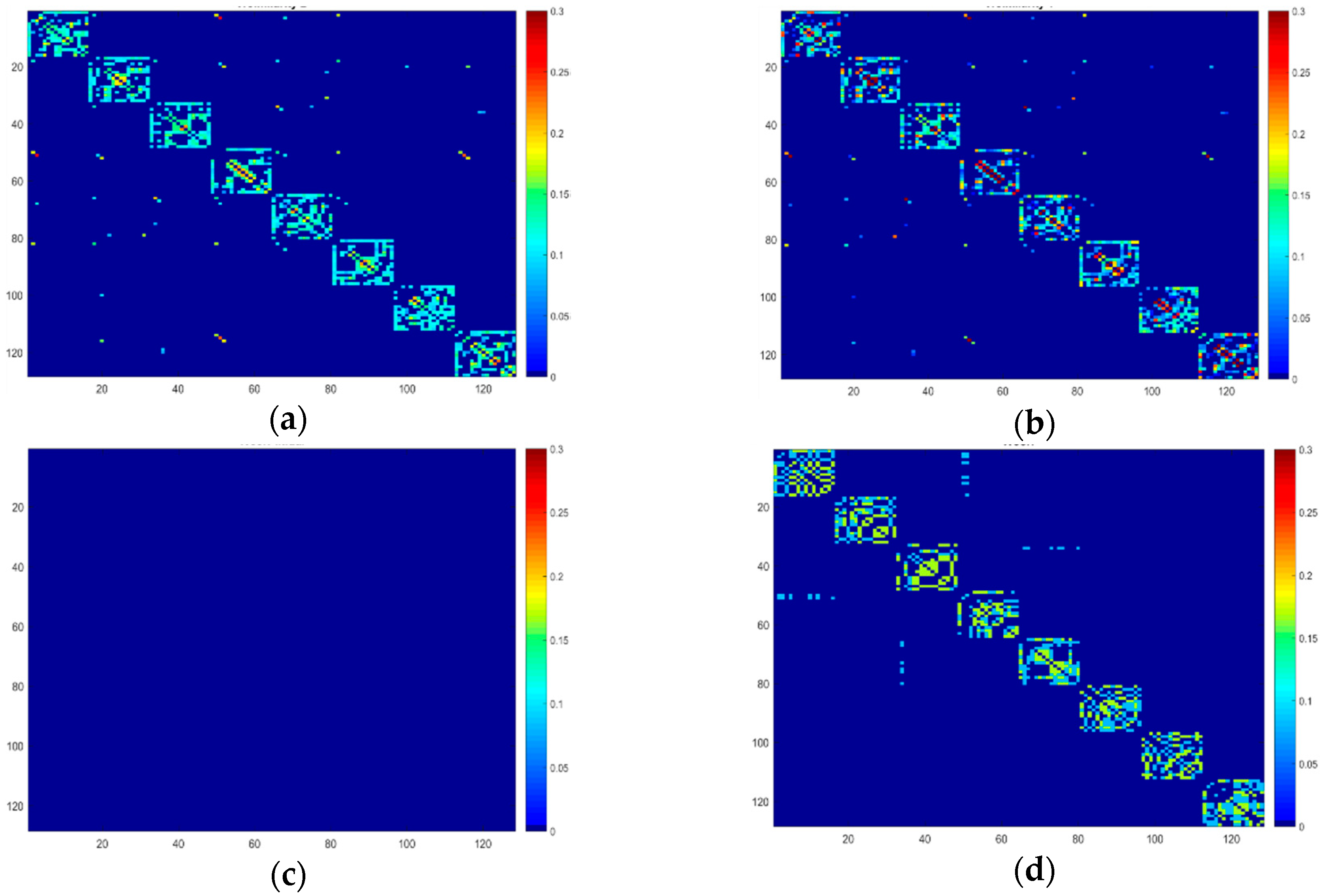
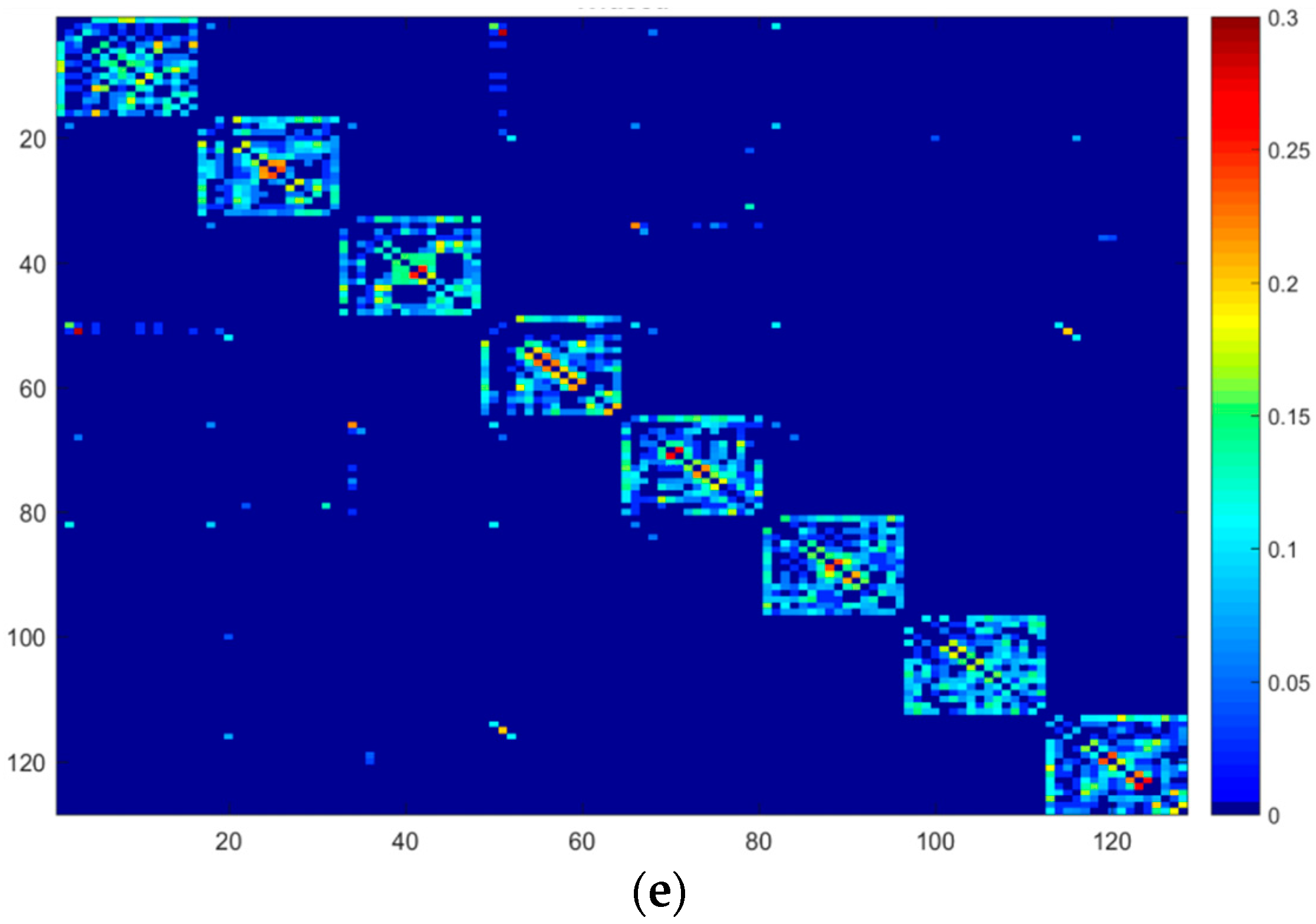
To illustrate the influence of our fusion method, we opted 17 samples from the first 8 classes of PF01 face database. In the feature extraction step, we fed the images into the VGG Face deep network and extracted the information in layer 6, which was a fully connected layer (we called it FC6). One sample in each class was selected as the labeled data and the rest as unlabeled data. The data were placed close to each other, such that the samples of each class were alongside each other. Figure 3a,b exhibit the similarity between only the unlabeled samples based on the FC6 descriptor obtained by Adaptive k-NN graph and k-NN graph, respectively, both with K = 6. Before the LP, the similarity values of unlabeled data are zeros, so the similarity graph of the unlabeled part was plotted with the blue color that presents the 0 value on Figure 3c. After LP by FME, we used the labels of unlabeled samples to find the similarity between the nodes, Figure 3d is the correlation graph between the labels after 10 iterations of LP. Figure 3e shows the fusion graph associated with three graphs. As we observed, the fusion graph can amplify the strong similarity values and weaken the slight similarity values. Furthermore, we observed that the edge weight of inter-class nodes had high values (red colors), whereas the intra-class nodes had very small values (blue color), which is desirable behavior.

4.3. Comparison with Other Methods

In this part, we compared our proposed method with four state-of-the-art methods, named MLGC [32], MDLP [28], DGFLP [25], and SMGI [24]. To have a fair comparison, we used the same graphs as before for all methods. According to Reference [24], the parameters of SMGI were tuned as the maximum number of iteration to 100, λ₁ = 0.01, λ₂ = 0.1, and stopping condition was 1e⁻⁴. For the other algorithms, the optimum parameter was set to those which provide the highest accuracy on the FERET dataset. For MLGC, the optimal number of iterations was set to 20 from the range of Reference [1,25] and λ = 0.1 from the set of [0.01,0.1,0.5,1], and for DGFLP the number of optimal iterations was set to 20 from the range of Reference [1,25]. Finally, for MDLP, we set the parameters as K = 10, α = 0.3, λ = 1 among the set of K = [6,10,15,20], α, λ = [0.01,0.1,0.5,1] and the number of iterations set to six from the Reference [1,20].

Similar to the previous experiment, we set the number of labeled samples per class to one and two. The obtained results based on VGG Face-FC7 and VGG Face-FC6 descriptors were reported in

Table 4. Mean accuracy and standard deviation of the accuracy of the proposed method compared with other methods based on VGG Face-FC7 and VGG Face-FC6 features. DGFLP = dynamic graph fusion label propagation; SMGI = sparse multiple graph integration; MLGC = multi-view local and global consistency; MDLP = multi-modality dynamic label propagation.

Dataset	Method	Accuracy (Mean ± STD)
		FC7	FC6
PF01 1 labeled sample	SMGI	80.33 ± 13.01	78.12 ± 15.87
	MLGC	80.01 ± 12.84	77.83 ± 15.69
	DGFLP	80.54 ± 13.3	78.14 ± 15.72
	MDLP	76.29 ± 17.07	74.71 ± 19.12
	Proposed method	92.42 ± 2.86	93.99 ± 0.85
PF01 2 labeled samples	SMGI	88.12 ± 2.4	87.31 ± 3.35
	MLGC	87.79 ± 2.39	87.07 ± 3.39
	DGFLP	88.33 ± 2.72	87.4 ± 3.59
	MDLP	85.55 ± 1.82	85.42 ± 2.81
	Proposed method	94.36 ± 1.19	94.75 ± 0.98
Extended_Yale 1 labeled sample	SMGI	37.62 ± 19.08	39.28 ± 18.94
	MLGC	37.11 ± 17.93	39.56 ± 17.98
	DGFLP	37.93 ± 19.14	39.8 ± 19.21
	MDLP	29.21 ± 19.55	31.24 ± 20.2
	Proposed method	43.5 ± 19.34	50.38 ± 19.27
Extended_Yale 2 labeled samples	SMGI	48.87 ± 18.32	51.48 ± 18.64
	MLGC	47.72 ± 17.68	50.87 ± 18.12
	DGFLP	49.57 ± 18.61	51.96 ± 19.02
	MDLP	42.6 ± 18.56	45.57 ± 19.01
	Proposed method	55.35 ± 21.68	58.68 ± 21.77
PIE 1 labeled sample	SMGI	67.71 ± 9.07	63.03 ± 12.48
	MLGC	66.46 ± 8.72	62.12 ± 12.62
	DGFLP	68.96 ± 9.17	63.59 ± 12.22
	MDLP	63.01 ± 10.54	60.04 ± 12.83
	Proposed method	79.04 ± 8.21	79.77 ± 8.81
PIE 2 labeled samples	SMGI	77.65 ± 6.26	74.57 ± 7
	MLGC	76.16 ± 6.24	73.47 ± 6.95
	DGFLP	79.06 ± 6.65	75.54 ± 7.46
	MDLP	73.39 ± 6.71	70.11 ± 7.95
	Proposed method	88.35 ± 5.5	87.21 ± 5.9
FERET 1 labeled sample	SMGI	98.38 ± 0.25	98.56 ± 0.24
	MLGC	98.25 ± 0.3	98.52 ± 0.31
	DGFLP	98.43 ± 0.13	98.55 ± 0.13
	MDLP	96.32 ± 0.72	97.12 ± 0.4
	Proposed method	98.83 ± 0.08	99.03 ± 0.13
FERET 2 labeled samples	SMGI	98.71 ± 0.29	98.9 ± 0.32
	MLGC	98.49 ± 0.39	98.82 ± 0.31
	DGFLP	98.65 ± 0.43	98.8 ± 0.37
	MDLP	97.01 ± 0.49	97.5 ± 0.86
	Proposed method	98.99 ± 0.3	99.13 ± 0.26

and for LBP feature descriptor in

Table 5. Mean accuracy and standard deviation of the proposed method compared with other methods on LBP feature descriptor.

Accuracy (Mean ± STD)
	SMGI	MLGC	DGFLP	MDLP	Proposed Method
PF01	47.66 ± 10.94	46.55 ± 11.37	47.82 ± 11.1	17.47 ± 11.25	56.19 ± 8.97
1 labeled sample
PF01	56.77 ± 7.16	55.83 ± 7.82	56.9 ± 7.23	13.7 ± 10.58	65.47 ± 5.86
2 labeled samples
Extended_Yale	73.48 ± 10.52	58.29 ± 11	80.77 ± 9.98	12.34 ± 20.31	94.25 ± 1.52
1 labeled sample
Extended_Yale	80.05 ± 4.79	65.18 ± 6.87	86.73 ± 5.21	7.01 ± 11.61	96.73 ± 1.93
2 labeled samples
PIE	36 ± 5.9	34 ± 5.51	36.09 ± 5.58	16.28 ± 5.12	46.79 ± 7.36
1 labeled sample
PIE	49.84 ± 7.85	48.06 ± 7.72	50.65 ± 7.63	30.4 ± 9.86	61.64 ± 5.99
2 labeled samples

. With respect to the results of Table 4 and Table 5, we observed that the proposed method outperformed other fusion techniques adopting either deep or handcrafted features. Compared to the algorithms that use the correlation between the labels (i.e., DGFLP and MDLP), the proposed method obtained higher accuracy, which showed that the explicit use of the correlation information as a graph could improve the performance. Moreover, we observed that DGFLP algorithm had higher accuracy compared to MDLP. While both used the correlation graph, the former adopted unequal weights for the fusion of the graphs. As we mentioned, our method omitted the small and negative values that were obtained from the correlation of labels in order to remove the noisy values. Furthermore, it built a graph based on the correlation between the labels hence, its performance outperformed other methods.

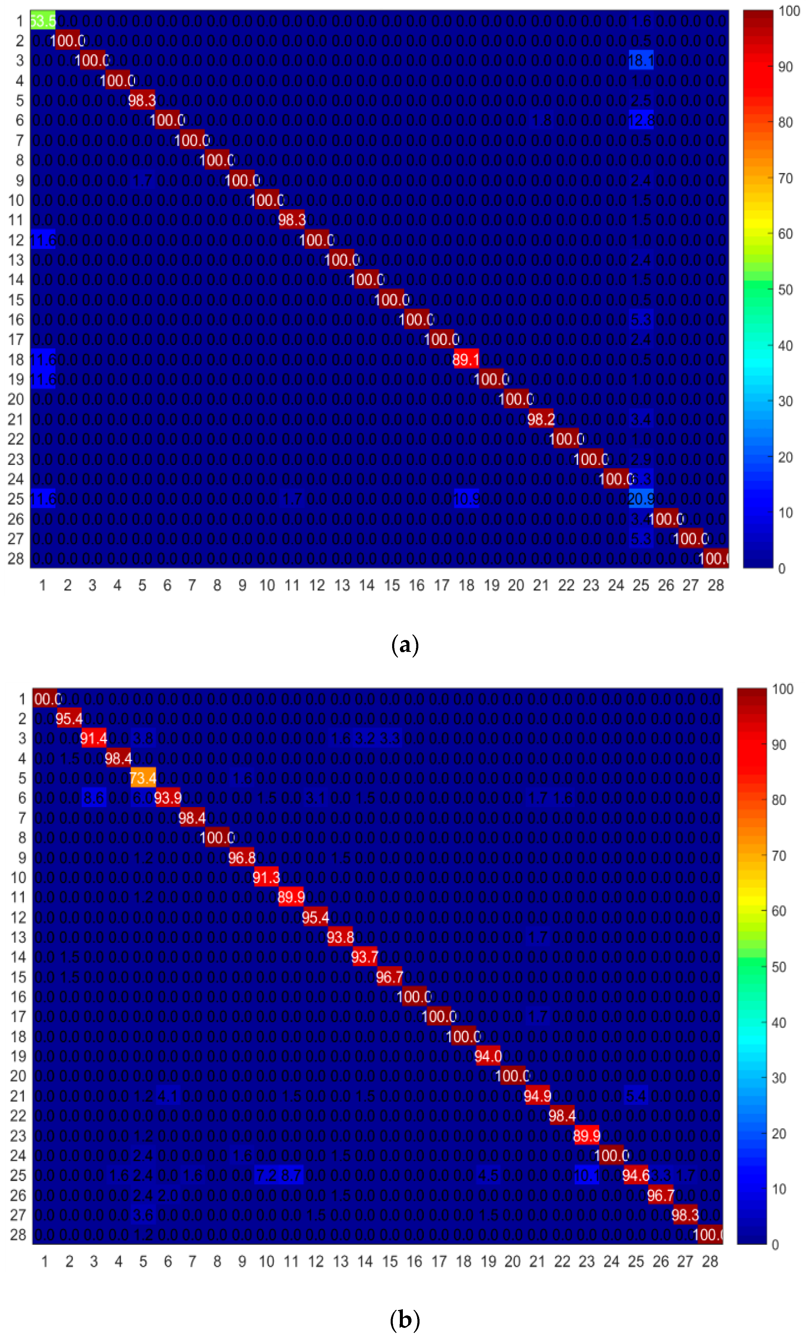
Moreover, we compared the confusion matrix of our proposed method with DGFLP method. For this test, we used the Extended Yale dataset which had 28 classes with LBP features and selected 1 sample in each class as the labeled data and the rest as the unlabeled data. In Figure 4, the horizontal axis demonstrates the target labels and the vertical axis shows the predicted labels. The warm color represents the high accuracy value and the cool color represents the low value of accuracy. Figure 4a is the confusion matrix of DGFLP method, and Figure 4b is the confusion matrix of our proposed method. As we observed, the confusion matrix of our proposed method was more uniform compared to that of DGFLP and had similar performance across different classes.

4.4. CPU-Time and Computational Complexity

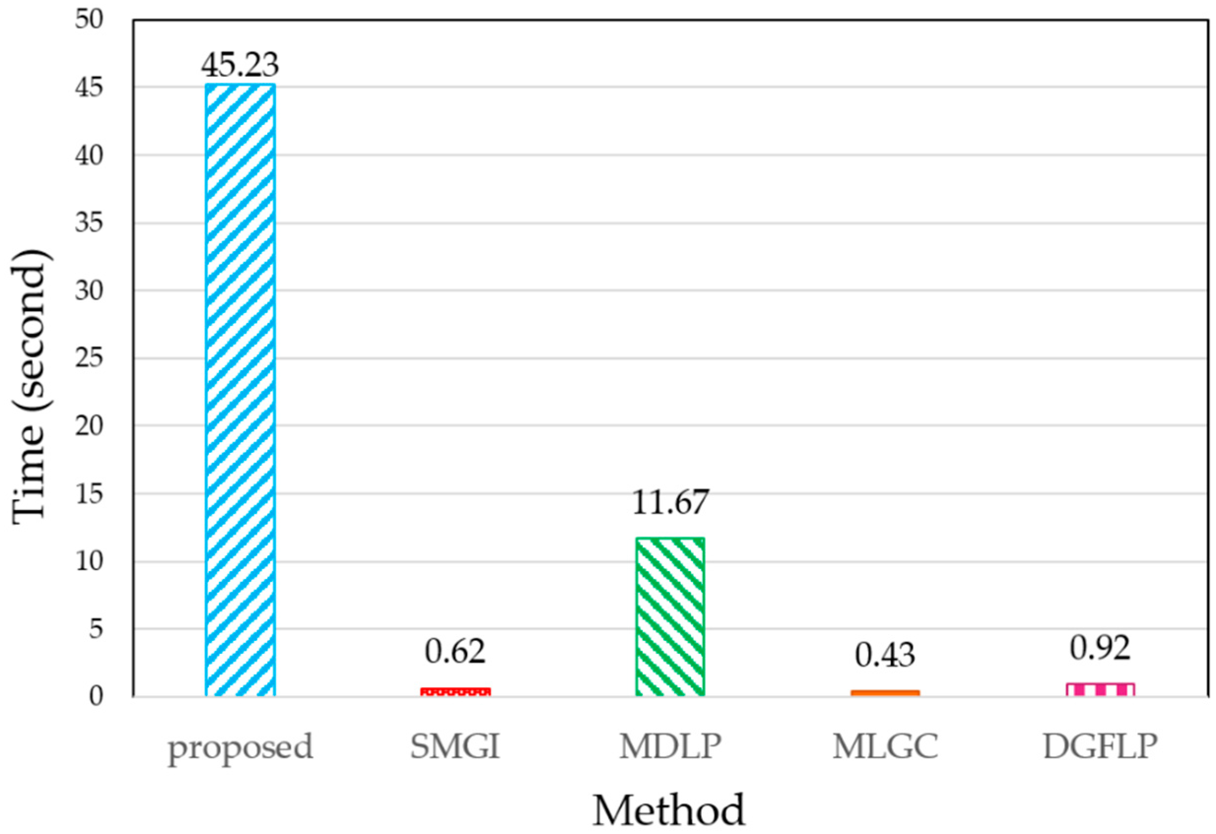
We also measured the running time of our method and that of other methods and plotted it in Figure 5. It is depicted from the average of 10 CPU elapsed time on PIE dataset based on the VGG Face-FC6 descriptor. The vertical axis demonstrates the time of CPU in seconds, and the horizontal axis shows the name of each method. As we can see, our method with 45.23 s had the greatest CPU time rather than other methods, but due to our accuracy results reported in Table 4, this computational time worth to be tolerated.

Moreover, since the computational complexity of FME is O(N³), the computational complexity of the proposed method will be O(T·N³) where T is the number of the adopted iterations.

5. Discussion and Conclusions

In this paper, we created multiple similarity metrics based on one feature descriptor and then fused the similarity graphs with equal weights to apply in the LP framework. We also used a new graph construction named correlation graph, based on the label space. In fact, we extended the FME algorithm into the multi-metric fusion method, to fuse multiple graphs based on the available feature and combining with the graph of the label space, to improve the accuracy of label propagation task. The experimental results on four face datasets showed that our multi-metric fusion method increased the accuracy compared to the use of a single feature. Indeed, we used the train part of the FME algorithm that assumed all the data were available at first. In the results, our method outperformed than other rival multi-graph fusion methods.

As a future work, we will try to assign unequal weight to each graph due to the available information of each one. Moreover, we envision the use of more than one view of data and the extraction of multiple feature descriptors to benefit multi-view information in graph fusion. Furthermore, the use of inductive setting of FME algorithm to estimate the labels of unseen data can be adopted to extend the proposed method to large scale databases. As we mentioned before, label propagation has different applications in community detection [16], image segmentation [17], and clustering [18], and classification [19] tasks. Therefore, in our future works, we will focus on applying the proposed method in the aforementioned applications. Moreover, since the proposed scenario of extracting information from the labels and creating a correlation graph is not limited to a specific label propagation method, any label propagation algorithm can benefit from the proposed scenario.

References

- Bashir, Y.; Aslam, A.; Kamran, M.; Qureshi, M.; Jahangir, A.; Rafiq, M.; Bibi, N.; Muhammad, N. On forgotten topological indices of some dendrimers structure. Molecules 2017, 22, 867. [Google Scholar] [CrossRef] [PubMed]
- Lu, J.; Hu, J.; Tan, Y.-P. Discriminative deep metric learning for face and kinship verification. IEEE Trans. Image Process. 2017, 26, 4269–4282. [Google Scholar] [CrossRef] [PubMed]
- Mirmahboub, B.; Mekhalfi, M.L.; Murino, V. Person re-identification by order-induced metric fusion. Neurocomputing 2018, 275, 667–676. [Google Scholar] [CrossRef]
- Zhang, H.; Huang, T.S.; Nasrabadi, N.M.; Zhang, Y. Heterogeneous Multi-Metric Learning for Multi-Sensor Fusion. In Proceedings of the 14th International Conference on Informatio Fusion (FUSION), Chicago, IL, USA, 5–8 July 2011; pp. 1–8. [Google Scholar]
- Zhang, L.; Zhang, D. Metricfusion: Generalized metric swarm learning for similarity measure. Inf. Fusion 2016, 30, 80–90. [Google Scholar] [CrossRef]
- Bai, J.; Xiang, S.; Pan, C. A graph-based classification method for hyperspectral images. IEEE Trans. Geosci. Remote Sens. 2013, 51, 803–817. [Google Scholar] [CrossRef]
- Boiman, O.; Shechtman, E.; Irani, M. In defense of nearest-neighbor based image classification. In Proceedings of the Conference on Computer Vision and Pattern Recognition (CVPR), Anchorage, AK, USA, 23–28 June 2008; pp. 1–8. [Google Scholar]
- Hartigan, J.A.; Wong, M.A. Algorithm as 136: A k-means clustering algorithm. J. R. Stat. Soc. 1979, 28, 100–108. [Google Scholar] [CrossRef]
- Vesanto, J.; Alhoniemi, E. Clustering of the self-organizing map. IEEE Trans. Neural Netw. 2000, 11, 586–600. [Google Scholar] [CrossRef] [PubMed] [Green Version]
- Von Luxburg, U. A tutorial on spectral clustering. Stat. Comput. 2007, 17, 395–416. [Google Scholar] [CrossRef] [Green Version]
- Zhang, L.; Qiao, L.; Chen, S. Graph-optimized locality preserving projections. Pattern Recognit. 2010, 43, 1993–2002. [Google Scholar] [CrossRef]
- Zhou, G.; Lu, Z.; Peng, Y. L1-graph construction using structured sparsity. Neurocomputing 2013, 120, 441–452. [Google Scholar] [CrossRef]
- Tang, J.; Hong, R.; Yan, S.; Chua, T.-S.; Qi, G.-J.; Jain, R. Image annotation by k nn-sparse graph-based label propagation over noisily tagged web images. ACM Trans. Intell. Syst. Technol. 2011, 2, 14:1–14:16. [Google Scholar] [CrossRef]
- Wang, F.; Zhang, C. Label propagation through linear neighborhoods. IEEE Trans. Knowl. Data Eng. 2008, 20, 55–67. [Google Scholar] [CrossRef]
- Gong, C.; Tao, D.; Maybank, S.J.; Liu, W.; Kang, G.; Yang, J. Multi-modal curriculum learning for semi-supervised image classification. IEEE Trans. Image Process. 2016, 25, 3249–3260. [Google Scholar] [CrossRef] [PubMed]
- Zhang, X.-K.; Ren, J.; Song, C.; Jia, J.; Zhang, Q. Label propagation algorithm for community detection based on node importance and label influence. Phys. Lett. A 2017, 381, 2691–2698. [Google Scholar] [CrossRef]
- Breve, F. Interactive image segmentation using label propagation through complex networks. Expert Syst. Appl. 2019, 123, 18–33. [Google Scholar] [CrossRef]
- Seyedi, S.A.; Lotfi, A.; Moradi, P.; Qader, N.N. Dynamic graph-based label propagation for density peaks clustering. Expert Syst. Appl. 2019, 115, 314–328. [Google Scholar] [CrossRef]
- Cui, B.; Xie, X.; Hao, S.; Cui, J.; Lu, Y. Semi-supervised classification of hyperspectral images based on extended label propagation and rolling guidance filtering. Remote Sens. 2018, 10, 515–533. [Google Scholar] [CrossRef]
- Chapelle, O.; Schölkopf, B.; Zien, A. Semi-Supervised Learning; MIT Press: Cambridge, MA, USA, 2006; Chapter 11; ISBN 978-0-262-03358-9. [Google Scholar]
- Nie, F.; Xu, D.; Tsang, I.W.-H.; Zhang, C. Flexible manifold embedding: A framework for semi-supervised and unsupervised dimension reduction. IEEE Trans. Image Process. 2010, 19, 1921–1932. [Google Scholar] [PubMed]
- Zhou, D.; Bousquet, O.; Lal, T.N.; Weston, J.; Schölkopf, B. Learning with local and global consistency. In Proceedings of the 18th Conference on Advances in Neural Information Processing Systems (NIPS), Vancouver, BC, Canada, 13–16 December 2004; pp. 321–328. [Google Scholar]
- Zhu, X.; Ghahramani, Z.; Lafferty, J.D. Semi-supervised learning using gaussian fields and harmonic functions. In Proceedings of the 20th International Conference on Machine Learning (ICML-03), Washington, DC, USA, 21–24 August 2003; pp. 912–919. [Google Scholar]
- Karasuyama, M.; Mamitsuka, H. Multiple graph label propagation by sparse integration. IEEE Trans. Neural Netw. Learn. Syst. 2013, 24, 1999–2012. [Google Scholar] [CrossRef] [PubMed]
- Lin, G.; Liao, K.; Sun, B.; Chen, Y.; Zhao, F. Dynamic graph fusion label propagation for semi-supervised multi-modality classification. Pattern Recognit. 2017, 68, 14–23. [Google Scholar] [CrossRef]
- Tong, T.; Gray, K.; Gao, Q.; Chen, L.; Rueckert, D. Alzheimer’s Disease Neuroimaging, I. Multi-modal classification of alzheimer’s disease using nonlinear graph fusion. Pattern Recognit. 2017, 63, 171–181. [Google Scholar] [CrossRef]
- Wang, B.; Mezlini, A.M.; Demir, F.; Fiume, M.; Tu, Z.; Brudno, M.; Haibe-Kains, B.; Goldenberg, A. Similarity network fusion for aggregating data types on a genomic scale. Nat. Methods 2014, 11, 333:1–333:8. [Google Scholar] [CrossRef] [PubMed]
- Wang, B.; Tsotsos, J. Dynamic label propagation for semi-supervised multi-class multi-label classification. Pattern Recognit. 2016, 52, 75–84. [Google Scholar] [CrossRef]
- Muhammad, N.; Bibi, N.; Qasim, I.; Jahangir, A.; Mahmood, Z. Digital watermarking using hall property image decomposition method. Pattern Anal. Appl. 2018, 21, 997–1012. [Google Scholar] [CrossRef]
- Muhammad, N.; Bibi, N. Digital image watermarking using partial pivoting lower and upper triangular decomposition into the wavelet domain. IET Image Process. 2015, 9, 795–803. [Google Scholar] [CrossRef]
- Li, S.; Liu, H.; Tao, Z.; Fu, Y. Multi-view graph learning with adaptive label propagation. In Proceedings of the IEEE International Conference on Big Data (Big Data), Boston, MA, USA, 11–14 December 2017; pp. 110–115. [Google Scholar]
- An, L.; Chen, X.; Yang, S. Multi-graph feature level fusion for person re-identification. Neurocomputing 2017, 259, 39–45. [Google Scholar] [CrossRef]
- Saeedeh, B.; Bosaghzadeh, A. Deep graph fusion for graph based label propagation. In Proceedings of the 10th Conference on Machine Vision and Image Processing (MVIP), Isfahan, Iran, 22–23 November 2017; pp. 149–153. [Google Scholar]
- Zhao, R.; Ouyang, W.; Wang, X. Person re-identification by salience matching. In Proceedings of the IEEE International Conference on Computer Vision, Sydney, Australia, 1–8 December 2013; pp. 2528–2535. [Google Scholar]
- Zhao, R.; Ouyang, W.; Wang, X. Unsupervised salience learning for person re-identification. In Proceedings of the IEEE Conference on Computer Vision and Pattern Recognition, Washington, DC, USA, 23–28 June 2013; pp. 3586–3593. [Google Scholar]
- Zhang, Y.; Zhang, H.; Nasrabadi, N.M.; Huang, T.S. Multi-metric learning for multi-sensor fusion based classification. Inf. Fusion 2013, 14, 431–440. [Google Scholar] [CrossRef]
- Wang, B.; Tu, Z.; Tsotsos, J.K. Dynamic label propagation for semi-supervised multi-class multi-label classification. In Proceedings of the IEEE International Conference on Computer Vision, Sydney Conference Centre, Darling Harbour, Sydney, 1–8 December 2013. [Google Scholar]
- Cortes, C.; Mohri, M. On transductive Regression. In Proceedings of the Conference on Neural Information Processing Systems (NIPS), Hyatt Regency Vancouver, Vancouver, BC, Canada, 3–8 December 2007. [Google Scholar]
- Yang, B.; Chen, S. Sample-dependent graph construction with application to dimensionality reduction. Neurocomputing 2010, 74, 301–314. [Google Scholar] [CrossRef]
- Bang, S.; Kim, D.; Choi, S. Asian Face Image Database PF01; Intelligent Multimedia Lab, University of Science and Technology: Pohang, Korea, 2001. [Google Scholar]
- Phillips, P.J.; Moon, H.; Rauss, P.; Rizvi, S.A. The feret evaluation methodology for face-recognition algorithms. In Proceedings of the Conference on IEEE Computer Society Conference on Computer Vision and Pattern Recognition, San Juan, Puerto Rico, USA, 17–19 June 1997. [Google Scholar]
- Parkhi, O.M.; Vedaldi, A.; Zisserman, A. Deep face recognition. In Proceedings of the BMVC, Swansea, UK, 7–10 September 2015; p. 6. [Google Scholar]
- Ojala, T.; Pietikainen, M.; Maenpaa, T. Multiresolution gray-scale and rotation invariant texture classification with local binary patterns. IEEE Trans. Pattern Anal. Mach. Intell. 2002, 24, 971–987. [Google Scholar] [CrossRef] [Green Version]
Figure 1.
The framework of the proposed method. The available view of data is demonstrated in green color. Different graphs are created according to available data. The brown-colored graph is built on the view of the label space. All the graphs are fused. The resulted graph is given to the flexible manifold embedding (FME) algorithm. In the final iteration, the projection matrix and bias vector are used for predicting the labels of the unseen data.
Figure 2.
The flowchart of the proposed method.
Figure 3.
The similarity matrix of unlabeled data from the PF01 dataset with eight classes and one sample from each class selected as the labeled data. (a) The similarity matrix of Adaptive k-NN graph based on VGG Face-FC6 with K = 6. (b) The similarity matrix of k-NN graph based on VGG Face-FC6 with K = 6 and σ = 0.05. (c) The similarity matrix of correlation graph based on VGG Face-FC6 with K = 6, which is before LP. (d) The similarity matrix of the correlation graph after 10 iterations of LP. (e) The similarity matrix of the fused graph.
Figure 4.
Confusion matrix of our proposed method and DGFLP method on the Extended Yale dataset on LBP features, where (a) is the confusion matrix of DGFLP method and (b) is the confusion matrix of our proposed method.
Figure 5.
The mean of runtime on PIE dataset for the SMGI, MDLP, MLGC, DGFLP, and our proposed method based on VGG Face-FC6.