Extreme Multiclass Classification Criteria


NYU Tandon School of Engineering, Department of Electrical and Computer Engineering 5 MetroTech Center, Brooklyn, NY 11201, USA
*
Author to whom correspondence should be addressed.
Computation 2019, 7(1), 16; https://0-doi-org.brum.beds.ac.uk/10.3390/computation7010016
Submission received: 2 February 2019
/
Revised: 5 March 2019
/
Accepted: 8 March 2019
/
Published: 12 March 2019
(This article belongs to the Special Issue Machine Learning for Computational Science and Engineering)
Abstract
:We analyze the theoretical properties of the recently proposed objective function for efficient online construction and training of multiclass classification trees in the settings where the label space is very large. We show the important properties of this objective and provide a complete proof that maximizing it simultaneously encourages balanced trees and improves the purity of the class distributions at subsequent levels in the tree. We further explore its connection to the three well-known entropy-based decision tree criteria, i.e., Shannon entropy, Gini-entropy and its modified variant, for which efficient optimization strategies are largely unknown in the extreme multiclass setting. We show theoretically that this objective can be viewed as a surrogate function for all of these entropy criteria and that maximizing it indirectly optimizes them as well. We derive boosting guarantees and obtain a closed-form expression for the number of iterations needed to reduce the considered entropy criteria below an arbitrary threshold. The obtained theorem relies on a weak hypothesis assumption that directly depends on the considered objective function. Finally, we prove that optimizing the objective directly reduces the multi-class classification error of the decision tree.
1. Introduction
This paper focuses on the multiclass classification setting, where the number of classes is very large. The recent widespread development of data-acquisition web services and devices has helped make large data sets, such as multiclass data sets, commonplace. Straightforward extensions of the binary approaches to the multiclass setting, such as the one-against-all approach [1], which for each data point computes a score for each class and returns the class with the maximum score, do not often work in the presence of strict computational constraints as their running time often scales linearly with the number of labels k. On the other hand, the most computationally efficient approaches for multiclass classification are given by train/test running time [2]. This running time can naturally be achieved by hierarchical classifiers that build the hierarchy over the labels.
This paper considers a hierarchical multiclass decision tree structure, where each node of the tree contains a binary classifier h from some hypothesis class that sends an example reaching that node to either left () or right () child node depending on the sign of (each node has its own splitting hypothesis). The test example descends from the root to the leaf of such tree guided by the classifiers lying on its path, and is labeled according to the label with the highest frequency amongst the training examples that were reaching the leaf that it descended to. The tree is constructed and trained in a top-down fashion, where splitting the data in every node of the tree is done by maximizing the following objective function recently introduced in the literature [3] (along with the algorithm (we refer the reader to the referenced paper for the algorithm’s details), called LOMtree, optimizing it in an online fashion):
where are the data points (each with a label from the set ), denotes the proportion of label i amongst the examples reaching a node, and probabilities and denote the fraction of examples reaching a node for which , marginally and conditional on class i respectively. The objective measures the dependence between the split and the class distribution. Note that it satisfies and, as implied by its form, maximizing it encourages the fraction of examples going to the right from class i to be substantially different from the background fraction for each class i. Thus for a balanced split (i.e., ), the examples of class i are encouraged to be sent exclusively to the left () or right () refining the purity of the class distributions at subsequent levels in the tree. The LOMtree algorithm effectively maximizes this objective over hypotheses in an online fashion with stochastic gradient descent (SGD) and obtains good-quality multiclass tree predictors with logarithmic train and test running times. Despite that, this objective and its properties (including the relation to the more standard entropy criteria) remain largely ununderstood. Its exhaustive analysis is instead provided in this paper.
Our contributions are the following:
- We provide an extensive theoretical analysis of the properties of the considered objective and prove that maximizing this objective in any tree node simultaneously encourages balanced partition of the data in that node and improves the purity of the class distributions at its children nodes.
- We show a formal relation of this objective to some more standard entropy-based objectives, i.e., Shannon entropy, Gini-entropy and its modified variant, for which online optimization schemes in the context of multiclass classification are largely unknown. In particular we show that i) the improvement in the value of entropy resulting from performing the node split is lower-bounded by an expression that increases with the value of the objective and thus ii) the considered objective can be used as a surrogate function for indirectly optimizing any of the three considered entropy-based criteria.
- We present three boosting theorems for each of the three entropy criteria, which provide the number of iterations needed to reduce each of them below an arbitrary threshold. Their weak hypothesis assumptions rely on the considered objective function.
- We establish the error bound that relates maximizing the objective function with reducing the multi-class classification error.
- Finally, in the Appendix A we establish an empirical connection between the multiclass classification error and the entropy criteria and show that Gini-entropy most closely resembles the behavior of the test error in practice.
The main theoretical analysis of this paper is kept in the boosting framework [4] and relies on the assumption that the objective function can be weakly optimized in the internal nodes of the tree. This weak advantage is amplified in the tree leading to hierarchies achieving any desired level of entropy (either Shannon entropy, Gini-entropy or its modified variant). Our work adds new theoretical results to the theory of multiclass boosting. Note that the multiclass boosting is largely ununderstood from the theoretical perspective [5] (we refer the reader to [5] for comprehensive review of the theory of muticlass boosting).
The paper is organized as follows: related literature is discussed in Section 2, the theoretical properties of the objective are shown in Section 3, the main theoretical results are presented in Section 4, and finally the mathematical properties of the entropy criteria and the proofs of the main theoretical results are provided in Section 5. Conclusions (Section 6) end the paper. Appendix A contains basic numerical experiments (Appendix A.1) and additional proofs (Appendix A.2).
2. Related Work
The extreme multiclass classification problem has been addressed in the literature in different ways. We discuss them here, putting emphasis on the ones that build hierarchical predictors as these techniques are the most relevant to this paper. Only a few authors [2,3,6,7,8] simultaneously address logarithmic time training and testing. The methods they propose are either hard to apply in practical problems [7] or use fixed tree structures [6,8]. Furthermore, an alternative approach based on using a random tree structure was shown to potentially lead to considerable underperformance [3,9]. At the same time, for massive datasets making multiple passes through the data is computationally costly, which justifies the need for developing online approaches, where the algorithm streams over a potentially infinitely large data set (online approaches are also plausible for non-stationary problems). It is unclear how to optimize standard decision tree objectives, such as Shannon or Gini-entropy, in this setting (early attempt was recently proposed [2] for Shannon entropy). One of the prior works to this paper [3] introduces an objective function which enjoys certain advantages over entropy criteria. In particular, it can be easily and efficiently optimized online. The authors however present an incomplete theoretical analysis and leave a number of open questions, which this paper instead aims at addressing. The algorithms for incremental learning of classification with decision trees also include some older works [10,11,12], which split any node according to the outcome of the node split-test based on the values of selected attributes of the data examples reaching that node. These approaches are different from the one in this paper, where the node split is performed according to the value of the learned (e.g., with SGD) hypothesis computed for the entire vector of attributes of the data examples reaching that node.
Other tree-based approaches include conditional probability trees [13] and clustering methods [9,14,15] ([9] was later improved in [16]), but they allow training time to be linear in the label complexity. The remaining techniques for multiclass classification include sparse output coding [17], variants of error correcting output codes [18], variants of iterative least-squares [19], and a method based on guess-averse loss functions [20].
Finally note that the conditional density estimation problem is also challenging in the large-class settings and in this respect remains parallel to the extreme multiclass classification problem [21]. In the context of conditional density estimation problem, there have also been some works that use tree structured models to accelerate computation of the likelihood and gradients [8,22,23,24]. They typically use heuristics based on using ontologies [8], Huffman coding [24], and various other mechanisms.
3. Theoretical Properties of the Objective Function
In this section we describe the objective function introduced in Equation (1) and provide its theoretical properties. The proofs are deferred to the Appendix. We first introduce the definitions of the concept of balancedness and purity of the node split.
Definition 1 (Purity and balancedness).
The hypothesis induces a pure split if , where , and α is called the purity factor.
The hypothesis induces a balanced split if , where , and β is called the balancing factor.
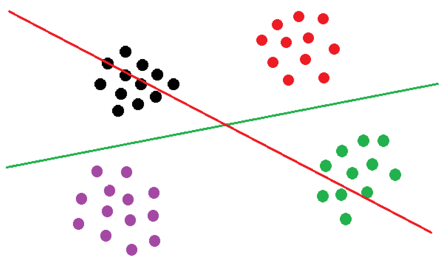
A partition is perfectly pure if (examples of the same class are sent exclusively to the left or to the right). A partition is called perfectly balanced if (equal number of examples are sent to the left and to the right). The notions of balancedness and purity are conveniently illustrated in Figure 1, where it is shown that the purity criterion helps to refine the choice of the splitting hypothesis from among well-balanced candidates.
Next, we show the first theoretical property of the objective function that characterizes its behavior at the optimum ().
Lemma 1.
The hypothesis induces a perfectly pure and balanced partition if and only if .
For some data sets however there exist no hypotheses producing perfectly pure and balanced splits. We next show that increasing the value of the objective leads to more balanced splits.
Lemma 2.
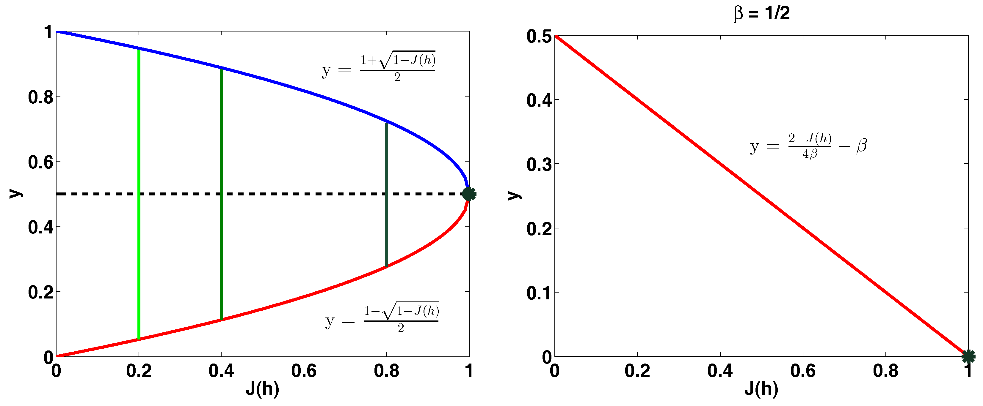
For any hypothesis h and any distribution over data examples the balancing factor β satisfies .
We refer to the interval to which belongs to as -interval. Thus the larger (closer to 1) the value of is, the narrower the -interval is, leading to more balanced splits at the extremes of this interval ( closer to ).
This result combined with the next lemma implies that, at the extremes of the interval, the value of the upper-bound on the purity factor decreases as the value of increases (since gets closer to 1 and the balancing factor gets closer to at the extremes of the interval). The recovered splits therefore have better purity ( closer to 0).
Lemma 3.
(Lemma 1 in [3]). For any hypothesis h and any distribution over data examples the purity factor α and the balancing factor β satisfy .
Note that the equality condition in Lemma 3 is achieved when (and thus, , , and ).
We thus showed that maximizing the objective in Equation (1) in each tree node simultaneously encourages trees that are balanced and whose purity of the class distributions is gradually improving when moving from the root to a subsequent tree levels. Lemmas 2 and 3 are illustrated in Figure 2.
In the next section we show that the objective is related to the more standard decision tree entropy-based objectives and that maximizing it leads to the reduction of these criteria. We consider three different entropy criteria in this paper. The theoretical analysis relies on the boosting framework and depends on the weak learning assumption. Three different entropy-based criteria lead to three different theoretical statements, where we bound the number of splits required to reduce the value of the criterion below given level. The bounds we obtain, and their dependences on the number of classes (k), critically depend on the strong concativity properties of the considered entropy-based objectives.
4. Main Theoretical Results
4.1. Notation
We first introduce notation. Let denote the tree under consideration. ’s denote the probabilities that a randomly chosen data point x drawn from , where is a fixed target distribution over , has label i given that x reaches node l (note that ), t denotes the number of internal tree nodes, denotes the set of all tree leaves at time t, and is the weight of leaf l defined as the probability a randomly chosen x drawn from reaches leaf l (note that ). We study a tree construction algorithm where we recursively find the leaf node with the highest weight, and choose to split it into two children. Consider the tree constructed over t steps where in each step we take one leaf node and split it (thus the number of splits is equal to the number of internal nodes of the tree) ( corresponds to splitting the root, thus the tree consists of one node (root) and its two children (leaves) in this step). We measure the quality of the tree at any given time t with three different entropy criteria:
- Shannon entropy :
- Gini-entropy :
- Modified Gini-entropy :where is a constant such that .
These criteria are the natural extensions of the criteria used in the context of binary classification [25] to the multiclass classification setting (note that there is more than one way of extending the entropy-based criteria from [25] to the multiclass classification setting, e.g., the modified Gini-entropy could as well be defined as , where . This and other extensions will be investigated in future works). We will next present the main results of this paper, which will be followed by their proofs. We begin with introducing the weak hypothesis assumption.
4.2. Theorems
Definition 2 (Weak Hypothesis Assumption).
Let m denote any internal node of the tree , and let and . Furthermore, let be such that for all m, . We say that the weak hypothesis assumption is satisfied when for any distribution over at each node m of the tree there exists a hypothesis such that .
The weak hypothesis assumption says that in every node of the tree we are able to recover a hypothesis from which corresponds to the value of the objective that is above 0 (thus the corresponding split is “weakly” pure and “weakly” balanced).
Consider next any time t and let n be the heaviest leaf at time t that we split and its weight be denoted by w for brevity. Similarly, let h denote the regressor at node n (shorthand for ). We denote the difference between the contribution of node n to the value of the entropy-based objectives in times t and as
Then the following lemma holds (the proof in provided in Section 5):
Lemma 4.
Under the Weak Hypothesis Assumption, the change in entropies occuring due to the node split can be bounded as
Clearly, maximizing the objective improves the entropy reduction. The considered objective can therefore be viewed as a surrogate function for indirectly optimizing any of the three considered entropy-based criteria, for which efficient online optimization strategies are largely unknown but highly desired in the multiclass classification setting. To be more specific, the standard packages for binary classification trees, such as CART [26] and C4.5 [27], require running a brute force search to find a partition at every node of the tree from a set of all possible partitions that leads to the biggest improvement of the entropy-based criterion of interest [25]. This is prohibitive in case of the multiclass problem. however can be efficiently optimized with SGD instead.
We next state the three boosting theoretical results captured in Theorems 1–3. They guarantee that the top-down decision tree algorithm which optimizes in each node will amplify the weak advantage, captured in the weak learning assumption, to build a tree achieving any desired level of entropy (either Shannon entropy, Gini-entropy or its modified variant).
Theorem 1.
Under the Weak Hypothesis Assumption, for any , to obtain it suffices to make splits.
Theorem 2.
Under the Weak Hypothesis Assumption, for any , to obtain it suffices to make splits.
Theorem 3.
Under the Weak Hypothesis Assumption, for any , to obtain it suffices to make splits.
Finally, we provide the error guarantee in Theorem 4. Denote to be a fixed target function with domain , which assigns the data point x to its label, and let be a fixed target distribution over . Together y and induce a distribution on labeled pairs . Let be the label assigned to data point x by the tree. We denote as the error of tree , i.e.,
Theorem 4.
Under the Weak Hypothesis Assumption, for any , to obtain it suffices to make splits.
Remark 1.
The main theorems show how fast the entropy criteria or the multi-class classification error drop as the tree grows and performs node splits. These statements therefore provide a platform for comparing different entropy criteria and answer two questions: 1) for a fixed , and k, which criterion is reduced the most with each split? and 2) can the multi-class error match the convergence speed of the best entropic criterion? Hence, it can be noted that the Shannon entropy has the most advantageous dependence on the label complexity, since the bound scales only logarithmically with k, and thus achieves the fastest convergence. Simultaneously, the multi-class classification rate matches this advantageous convergence rate and also scales favorably (logarithmically) with k. Finally, even though the weak hypothesis requires only slightly favorable γ, i.e., , in practice when constructing the tree one can optimize J in every node of the tree, which effectively pushes γ to be as high as possible. In that case γ becomes a well-behaving constant in the above theorems, ideally equal to , and does not negatively affect the split count.
We next discuss in details the mathematical properties of the entropy-based criteria, which are important to prove the above theorems.
5. Proofs
5.1. Properties of the Entropy-Based Criteria
Each of the presented entropy-based criteria has a number of useful properties that we give next, along with their proofs. We first give bounds on the values of the entropy-based functions. As before, let w be the weight of the heaviest leaf in the tree at time t.
5.1.1. Bounds on the Entropy-Based Criteria
Lemma 5.
The Shannon entropy function at time t is bounded as .
Lemma 6.
The Gini-entropy function at time t is bounded as .
Lemma 7.
The modified Gini-entropy function at time t is bounded as .
The upper-bounds in Lemmas 5–7 are tight, where the equalities hold for the special case when , e.g., when each internal node of the tree produce a perfectly pure and balanced split.
5.1.2. Strong Concativity Properties of the Entropy-Based Criteria
So far we have been focusing on the time step t. Recall that n is the heaviest leaf at time t and its weight is denoted by w for brevity. Consider splitting this leaf to two children and . For ease of notation let and , and , and furthermore let and h be the shorthands for and , respectively. Recall that and . Notice that and . Let be the k-element vector with entry equal to . Finally, let , , and . Before the split the contribution of node n to resp. , , and was resp. , , and . Note that and are the probabilities that a randomly chosen x drawn from has label i given that x reaches nodes and respectively. For brevity, let and be denoted respectively as and . Let be the k-element vector with entry equal to and let be the k-element vector with entry equal to . Notice that . After the split the contribution of the same, now internal, node n changes to resp. , , and . We can compute the difference between the contribution of node n to the value of the entropy-based objectives in times t and as
The next three lemmas, Lemmas 8–10, describe the strong concativity properties of the entropy, Gini-entropy and modified Gini-entropy, which can be used to lower-bound , , and (Equations (2)–(4) correspond to a gap in the Jensen’s inequality applied to the strongly concave function).
Lemma 8.
The Shannon entropy function is strongly concave with respect to -norm with modulus 1, and thus the following holds .
Lemma 9.
The Gini-entropy function is strongly concave with respect to -norm with modulus 2, and thus the following holds .
Lemma 10.
The modified Gini-entropy function is strongly concave with respect to -norm with modulus , and thus the following holds .
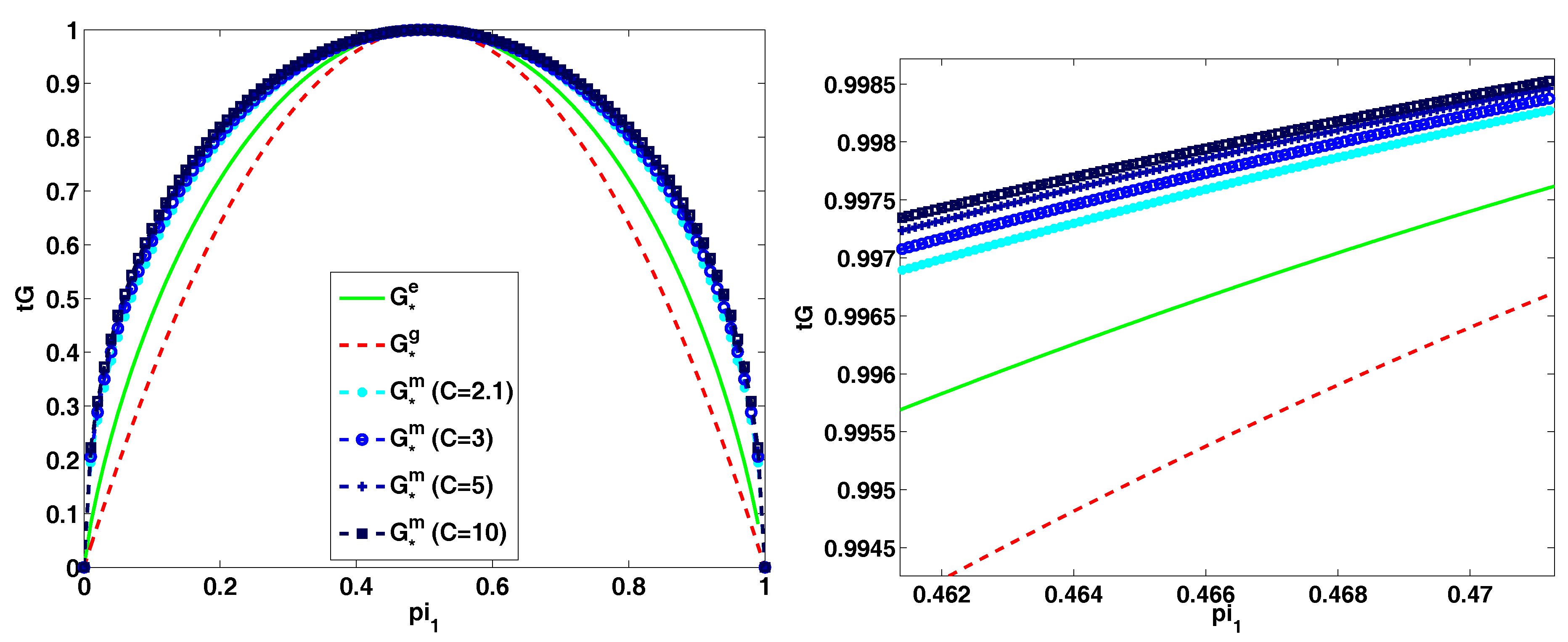
Figure 3 illustrates different entropy criteria normalized to the interval.
5.2. Proof of Lemma 4 and Theorems 1–3
We finally proceed to proving all three boosting theorems, Theorems 1–3. Lemma 4 is a by-product of these proofs.
Proof.
For the Shannon entropy it follows from Equation (2), Lemmas 5 and 8 that
where the last inequality comes from the fact that (see the definition of in the weak hypothesis assumption) and (see weak hypothesis assumption). For the Gini-entropy criterion notice that from Equation (3), Lemmas 6, 9, and A4 it follows that
where the last inequality is obtained similarly as the last inequality in Equation (5). And finally for the modified Gini-entropy it follows from Equation (4), Lemmas 7, 10, and A4 that
where the last inequality is obtained as before.
Clearly the larger the objective is at time t, the larger the entropy reduction ends up being. Let
For simplicity of notation assume corresponds to either , or , or , and stands for , or , or . Thus , and we obtain
One can now compute the minimum number of splits required to reduce below , where , from this recurrence inequality. Assume .
where . Recall that
where the last step follows from Lemma A5. Also note that by the same lemma . Thus,
Therefore to reduce (where ’s are defined in Theorems 1–3) it suffices to make splits such that splits. Since , where . Thus,
5.3. Proof of Theorem 4
We next proceed to directly proving the error bound. Recall that is the probability that the data point x corresponds to label i given that x reached l, i.e., . Let the label assigned to the leaf be the majority label and thus lets assume that the leaf is assigned to label i if and only if the following is true . Therefore we can write that
Let be the majority label in leaf l, thus . We can continue as follows
Consider again the Shannon entropy of the leaves of tree that is defined as
Note that
where the last inequality comes from the fact that and thus and consequently .
6. Conclusions
This paper aims at introducing theoretical tools, encapsulated in the boosting framework, that enable the comparison of different multi-class classification objective functions. The multi-class boosting is largely ununderstood from the theoretical perspective [5]. We provide an exhaustive theoretical analysis of the objective function underlying the recently proposed LOMtree algorithm for extreme multi-class classification and explore the connection of this objective to entropy-based criteria. We show that optimizing this objective simultaneously optimizes Shannon entropy, Gini-entropy and its modified variant, as well as the multi-class classification error. We expect that discussed tools can be used to obtain theoretical guarantees in the multi-label [28,29,30] and memory-constrained settings (we will explore this research direction in the future). We also consider extensions to different variants of the multi-class classification problem [31,32] and multi-output learning tasks [33,34]. We thus plan to build a unified theoretical framework for understanding extreme classification trees.
Author Contributions
A.C. derived the theoretical results and did the empirical evaluation. I.K.J. was working on improving the write-up of the paper and checking mathematical correctness.
Funding
This research received no external funding.
Conflicts of Interest
The authors declare no conflict of interest.
Appendix A. Extreme Multiclass Classification Criteria
Appendix A.1. Numerical Experiments
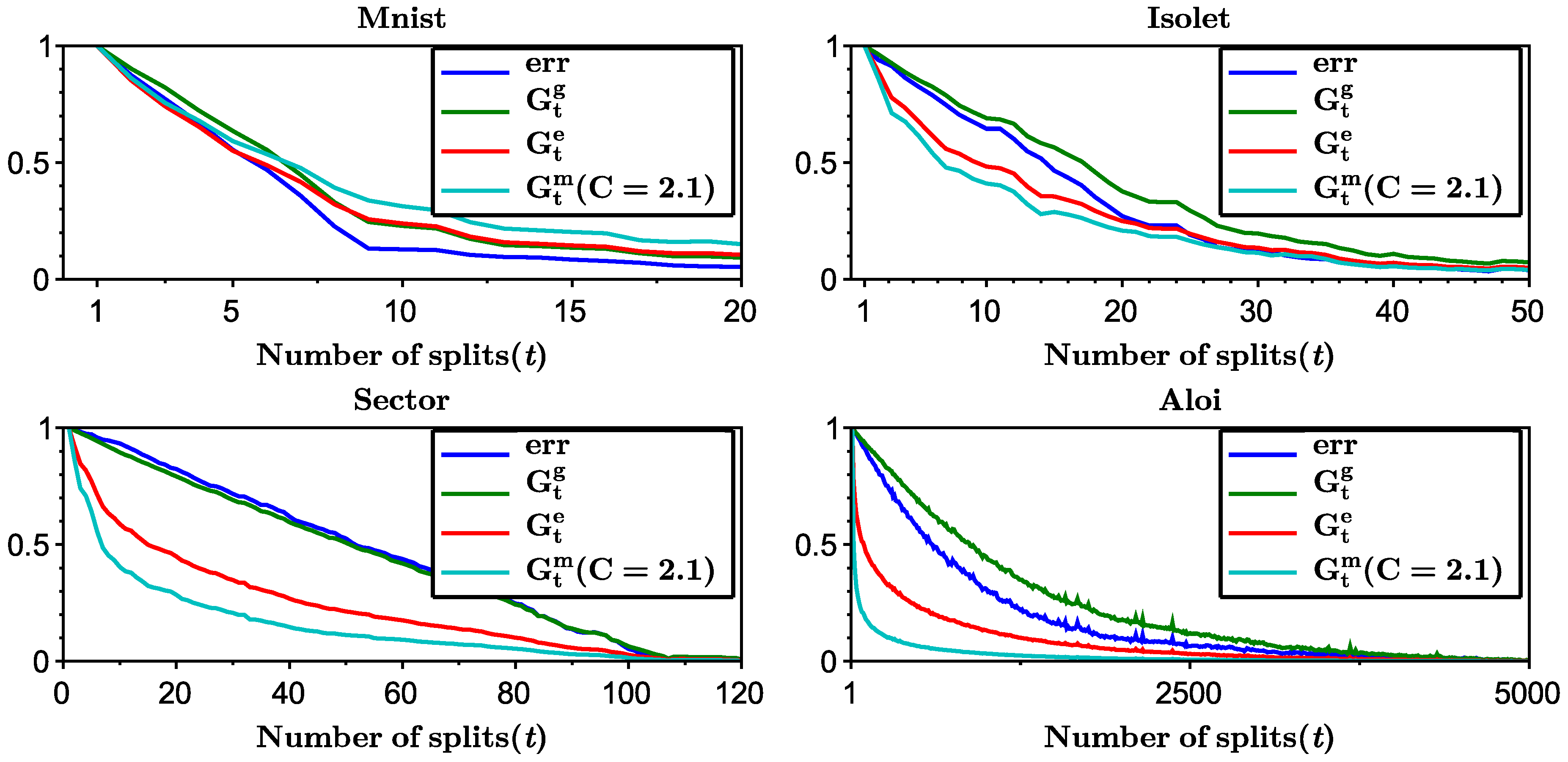
We run the LOMtree algorithm, which is implemented in the open source learning system Vowpal Wabbit [35], on four benchmark multiclass data sets: Mnist (10 classes, downloaded from http://yann.lecun.com/exdb/mnist/), Isolet (26 classes, downloaded from http://www.cs.huji.ac.il/~shais/datasets/ClassificationDatasets.html), Sector (105 classes, downloaded from http://www.csie.ntu.edu.tw/~cjlin/libsvmtools/datasets/multiclass.html), and Aloi (1000 classes, downloaded from http://www.csie.ntu.edu.tw/~cjlin/libsvmtools/datasets/multiclass.html). The data sets were divided into training () and testing (), where of the training data set was used as a validation set. The regressors in the tree nodes are linear and were trained by SGD [36] with 20 epochs and the learning rate chosen from the set . We investigated different swap resistances chosen from the set . We selected the learning rate and the swap resistance as the one minimizing the validation error, where the number of splits in all experiments was set to 10 k.
Figure A1 shows the Shannon entropy, Gini-entropy, modified Gini-entropy (all normalized to the interval ), and the multiclass classification error computed on the test data set as the function of the number of splits. The behavior of the Shannon entropy and Gini-entropy match the theoretical findings. However, the modified Gini-entropy instead drops the fastest with the number of splits, which in particular suggests that in this case perhaps tighter bounds could possibly be proved (for the binary case tighter analysis was shown in [25], but it is highly non-trivial to generalize this analysis to the multiclass classification setting). Furthermore, it can be observed that the behavior of the error closely mimics the behavior of the Gini-entropy. The Gini-entropy in all cases well-approximates the upper-bound on the error.
Figure A1.
Functions , , and , and the test error, all normalized to the interval , versus the number of splits. Figure is recommended to be read in color.
Figure A1.
Functions , , and , and the test error, all normalized to the interval , versus the number of splits. Figure is recommended to be read in color.

Appendix A.2. Additional Proofs
Proof of Lemma 1.
The proof that if h induces a maximally pure and balanced partition then was done in [3] (Lemma 2) and is very basic. We focus here on the remaining part of statement, which is harder to show, and prove that if then h induces a maximally pure and balanced partition.
Without loss of generality assume each . Recall that , and let . Also recall that . Thus . The objective is certainly maximized in the extremes of the interval , where each is either 0 or 1 (also note that at maximum, where , it cannot be that all ’s are 0 or all ’s are 1). The function is differentiable in these extremes ( is non-differentiable only when , but at considered extremes the left-hand side of this equality is in , whereas the right-hand side is either 0 or 1). We then write
where and . Also let (clearly and in the extremes of the interval where is maximized). We then can compute the derivatives of with respect to , where , everywhere where the function is differentiable as follows
and note that in the extremes of the interval where is maximized , since , , and each . Since is convex, and by the fact that in particular the derivative of with respect to any cannot be 0 in the extremes of the interval where is maximized, it follows that the can only be maximized () at the extremes of the interval. Thus we already proved that if then h induces a maximally pure partition. We are left with showing that if then h induces also a maximally balanced partition. We prove it by contradiction. Assume . Denote as before and . Recall . Thus,
where the last inequality comes from the fact that the quadratic form is equal to 1 only when , and otherwise it is smaller than 1. Thus we obtain the contradiction which ends the proof. □
Proof of Lemma 2.
We use the following notation: , and . Also let and . Recall that , and . We split the proof into two cases.
- Let . ThenThus which, when solved, yields the lemma.
- Let (thus ). Note that can be written assince and . Let , and . Note that and . Also note that . ThusThus as before we obtain which, when solved, yields the lemma. □
Proof of Lemma 5.
The lower-bound follows from the fact that the entropy of each leaf is non-negative. We next prove the upper-bound.
where the first inequality comes from the fact that uniform distribution maximizes the entropy, and the last equality comes from the fact that a tree with t internal nodes has leaves (also recall that w is the weight of the heaviest node in the tree at time t which is what we will also use in the next lemmas). □
Before proceeding to the actual proof of Lemma 6 we first introduce the helpful result captured in Lemma A1 and Corollary A1.
Lemma A1 (The inequality between Euclidean and arithmetic mean).
Let be a set of non-negative numbers. Then Euclidean mean upper-bounds the arithmetic mean as follows .
Corollary A1.
Let be non-negative. Then .
Proof.
By Lemma A1 we have . □
Proof of Lemma 6.
The lower-bound is straightforward since all ’s are non-negative. The upper-bound can be shown as follows (the last inequality results from Corollary A1):
□
Proof of Lemma 7.
The lower-bound can be shown as follows. Recall that the function is concave and therefore it is certainly minimized on the extremes of the interval, meaning where each is either 0 or 1. Let and let . Thus . Combining this result with the fact that gives the lower-bound. We next prove the upper-bound. Recall that Lemma A1 implies that , thus
By Jensen’s inequality . Thus
□
Proof of Lemma 8.
Lemma 8 is proven in [37] (Example 2.5). □
Lemma A2
(Lemma 14 in 38) If the function is twice differentiable, then the sufficient condition for strong concativity of Φ is that for all , , , where is the Hessian matrix of Φ at , and is the strong concativity modulus.
Proof of Lemma 9.
Note that , and apply Lemma A2. □
Lemma A3
(Remark 2.2.4. in 39) The sum of strongly concave functions on with modulus σ is strongly concave with the same modulus.
Proof of Lemma 10.
Consider functions , where , , and . Also let , where . It is easy to see, using Lemma A2, that function f is strongly concave with respect to -norm with modulus 2, thus
where and . Also note that h is strongly concave with modulus in its domain (the second derivative of h is ). The strong concativity of h implies that
where . Let and . Then we obtain
Note that
where the second inequality results from Equation (A1) and the last (third) inequality results from Equation (A2). Finally note that the first derivative of f is . Thus
and combining this result with previous statement yields
thus is strongly concave with modulus . By Lemma A3, is also strongly concave with the same modulus. □
The next two lemma are fundamental and they are used in the proof of Lemma 4 and the boosting theorems. The first one relates -norm and -norm and the second one is a simple property of the exponential function.
Lemma A4.
Let then .
Lemma A5.
For the following holds .
References
- Rifkin, R.; Klautau, A. In Defense of One-Vs-All Classification. J. Mach. Learn. Res. 2004, 5, 101–141. [Google Scholar]
- Daume, H.; Karampatziakis, N.; Langford, J.; Mineiro, P. Logarithmic Time One-Against-Some. arXiv, 2016; arXiv:1606.04988. [Google Scholar]
- Choromanska, A.; Langford, J. Logarithmic Time Online Multiclass prediction. In Neural Information Processing Systems 2015; Neural Information Processing Systems Foundation, Inc.: Vancouver, BC, Canada, 2015. [Google Scholar]
- Schapire, R.E.; Freund, Y. Boosting: Foundations and Algorithms; The MIT Press: Cambridge, MA, USA, 2012. [Google Scholar]
- Mukherjee, I.; Schapire, R.E. A theory of multiclass boosting. J. Mach. Learn. Res. 2013, 14, 437–497. [Google Scholar]
- Beygelzimer, A.; Langford, J.; Ravikumar, P.D. Error-Correcting Tournaments. In Algorithmic Learning Theory; Springer: Berlin/Heidelberg, Germany, 2009. [Google Scholar]
- Takimoto, E.; Maruoka, A. Top-down Decision Tree Learning As Information Based Boosting. Theor. Comput. Sci. 2003, 292, 447–464. [Google Scholar] [CrossRef]
- Morin, F.; Bengio, Y. Hierarchical probabilistic neural network language model. Aistats 2005, 5, 246–252. [Google Scholar]
- Bengio, S.; Weston, J.; Grangier, D. Label Embedding Trees for Large Multi-Class Tasks. In Advances in Neural Information Processing Systems 23 (NIPS 2010); NIPS: Vancouver, BC, Canada, 2010. [Google Scholar]
- Utgoff, P.E. Incremental Induction of Decision Trees. Mach. Learn. 1989, 4, 161–186. [Google Scholar] [CrossRef] [Green Version]
- Domingos, P.; Hulten, G. Mining High-speed Data Streams; KDD: Boston, MA, USA, 2000. [Google Scholar]
- Gama, J.; Rocha, R.; Medas, P. Accurate Decision Trees for Mining High-speed Data Streams. In Proceedings of the Ninth ACM SIGKDD International Conference on Knowledge Discovery and Data Mining, Washington, DC, USA, 24–27 August 2003. [Google Scholar]
- Beygelzimer, A.; Langford, J.; Lifshits, Y.; Sorkin, G.B.; Strehl, A.L. Conditional Probability Tree Estimation Analysis and Algorithms. In Proceedings of the Twenty-Fifth Conference on Uncertainty in Artificial Intelligence, Montreal, QC, Canada, 18–21 June 2009. [Google Scholar]
- Madzarov, G.; Gjorgjevikj, D.; Chorbev, I. A Multi-class SVM Classifier Utilizing Binary Decision Tree. Informatica 2009, 33, 225–233. [Google Scholar]
- Weston, J.; Makadia, A.; Yee, H. Label Partitioning For Sublinear Ranking. In Proceedings of the 30th International Conference on Machine Learning, Atlanta, GA, USA, 16–21 June 2013. [Google Scholar]
- Deng, J.; Satheesh, S.; Berg, A.C.; Fei-Fei, L. Fast and Balanced: Efficient Label Tree Learning for Large Scale Object Recognition. In Advances in Neural Information Processing Systems 24 (NIPS 2011); NIPS: Vancouver, BC, Canada, 2011. [Google Scholar]
- Zhao, B.; Xing, E.P. Sparse Output Coding for Large-Scale Visual Recognition. In Proceedings of the IEEE Conference on Computer Vision and Pattern Recognition (CVPR), Portland, OR, USA, 23–28 June 2013. [Google Scholar]
- Hsu, D.; Kakade, S.; Langford, J.; Zhang, T. Multi-Label Prediction via Compressed Sensing. In Advances in Neural Information Processing Systems 22 (NIPS 2009); NIPS: Vancouver, BC, Canada, 2009. [Google Scholar]
- Agarwal, A.; Kakade, S.M.; Karampatziakis, N.; Song, L.; Valiant, G. Least Squares Revisited: Scalable Approaches for Multi-class Prediction. In Proceedings of the 31st International Conference on Machine Learning (ICML 2014), Beijing, China, 21–26 June 2014. [Google Scholar]
- Beijbom, O.; Saberian, M.; Kriegman, D.; Vasconcelos, N. Guess-Averse Loss Functions For Cost-Sensitive Multiclass Boosting. In Proceedings of the 31st International Conference on Machine Learning (ICML 2014), Beijing, China, 21–26 June 2014. [Google Scholar]
- Jernite, Y.; Choromanska, A.; Sontag, D. Simultaneous Learning of Trees and Representations for Extreme Classification and Density Estimation. arXiv, 2017; arXiv:1610.04658. [Google Scholar]
- Mnih, A.; Hinton, G.E. A Scalable Hierarchical Distributed Language Model. In Advances in Neural Information Processing Systems 21 (NIPS 2008); NIPS: Vancouver, BC, Canada, 2009. [Google Scholar]
- Djuric, N.; Wu, H.; Radosavljevic, V.; Grbovic, M.; Bhamidipati, N. Hierarchical Neural Language Models for Joint Representation of Streaming Documents and their Content. In Proceedings of the 24th International Conference on World Wide Web, Florence, Italy, 18–22 May 2015. [Google Scholar]
- Mikolov, T.; Sutskever, I.; Chen, K.; Corrado, G.S.; Dean, J. Distributed representations of words and phrases and their compositionality. In Advances in Neural Information Processing Systems 26 (NIPS 2013); NIPS: Vancouver, BC, Canada, 2013. [Google Scholar]
- Kearns, M.; Mansour, Y. On the Boosting Ability of Top-Down Decision Tree Learning Algorithms. In Proceedings of the Twenty-Eighth Annual ACM Symposium on Theory of Computing (STOC ’96), Philadelphia, PA, USA, 22–24 May 1996. reprinted in J. Comput. Syst. Sci. 1999, 58, 109–128. [Google Scholar] [CrossRef]
- Breiman, L. Classification Regression Trees; Routledge: Abingdon, UK, 2017. [Google Scholar]
- Quinlan, J.R. C4.5: Programs for Machine Learning; Elsevier: Amsterdam, The Netherlands, 2014. [Google Scholar]
- Liu, W.; Tsang, I.W. Making decision trees feasible in ultrahigh feature and label dimensions. J. Mach. Learn. Res. 2017, 18, 2814–2849. [Google Scholar]
- Muñoz, E.; Nováček, V.; Vandenbussche, P.Y. Facilitating prediction of adverse drug reactions by using knowledge graphs and multi-label learning models. Brief. Bioinform. 2017, 20, 190–202. [Google Scholar] [CrossRef] [PubMed]
- Charte, F.; Rivera, A.J.; del Jesus, M.J.; Herrera, F. REMEDIAL-HwR: Tackling multilabel imbalance through label decoupling and data resampling hybridization. Neurocomputing 2019, 326, 110–122. [Google Scholar] [CrossRef]
- Koster, C.H.; Seutter, M.; Beney, J. Multi-classification of patent applications with Winnow. In International Andrei Ershov Memorial Conference on Perspectives of System Informatics; Springer: Berlin/Heidelberg, Germany, 2003; pp. 546–555. [Google Scholar]
- Liu, W.; Tsang, I.W.; Müller, K.R. An easy-to-hard learning paradigm for multiple classes and multiple labels. J. Mach. Learn. Res. 2017, 18, 3300–3337. [Google Scholar]
- Liu, W.; Xu, D.; Tsang, I.W.; Zhang, W. Metric learning for multi-output tasks. IEEE Trans. Pattern Anal. Mach. Intell. 2019, 41, 408–422. [Google Scholar] [CrossRef] [PubMed]
- Petersen, N.C.; Rodrigues, F.; Pereira, F.C. Multi-output bus travel time prediction with convolutional LSTM neural network. Expert Syst. Appl. 2019, 120, 426–435. [Google Scholar] [CrossRef]
- Langford, J.; Li, L.; Strehl, A. Vowpal Wabbit (Fast Learning). 2007. Available online: http://hunch.net/~vw (accessed on 2 February 2019).
- Bottou, L. Online Algorithms and Stochastic Approximations. In Online Learning and Neural Networks; Cambridge University Press: New York, NY, USA, 1998. [Google Scholar]
- Shalev-Shwartz, S. Online Learning and Online Convex Optimization. Found. Trends Mach. Learn. 2012, 4, 107–194. [Google Scholar] [CrossRef]
- Shalev-Shwartz, S. Online Learning: Theory, Algorithms, and Applications. Ph.D. Thesis, The Hebrew University of Jerusalem, Jerusalem, Israel, 2007. [Google Scholar]
- Zhukovskiy, V. Lyapunov Functions in Differential Games; Stability and Control: Theory, Methods and Applications; Taylor & Francis: London, UK, 2003. [Google Scholar]
Figure 1.
Red partition: highly balanced split but impure (the partition cuts through the black and green classes). Green partition: highly balanced and highly pure split. Figure should be read in color.
Figure 1.
Red partition: highly balanced split but impure (the partition cuts through the black and green classes). Green partition: highly balanced and highly pure split. Figure should be read in color.

Figure 2.
Left: Blue curve captures the behavior of the upper-bound on the balancing factor as a function of , red curve captures the behavior of the lower-bound on the balancing factor as a function of , green intervals correspond to the intervals where the balancing factor lies for different values of . Right: Red line captures the behavior of the upper-bound on the purity factor as a function of when the balancing factor is fixed to . Figure should be read in color.

Figure 3.
Functions , , and (functions , , and were re-scaled to have values in ) as a function of (). Figure should be read in color.
Figure 3.
Functions , , and (functions , , and were re-scaled to have values in ) as a function of (). Figure should be read in color.

© 2019 by the authors. Licensee MDPI, Basel, Switzerland. This article is an open access article distributed under the terms and conditions of the Creative Commons Attribution (CC BY) license (http://creativecommons.org/licenses/by/4.0/).
Share and Cite
MDPI and ACS Style
Choromanska, A.; Kumar Jain, I. Extreme Multiclass Classification Criteria. Computation 2019, 7, 16. https://0-doi-org.brum.beds.ac.uk/10.3390/computation7010016
AMA Style
Choromanska A, Kumar Jain I. Extreme Multiclass Classification Criteria. Computation. 2019; 7(1):16. https://0-doi-org.brum.beds.ac.uk/10.3390/computation7010016
Chicago/Turabian StyleChoromanska, Anna, and Ish Kumar Jain. 2019. "Extreme Multiclass Classification Criteria" Computation 7, no. 1: 16. https://0-doi-org.brum.beds.ac.uk/10.3390/computation7010016
Note that from the first issue of 2016, this journal uses article numbers instead of page numbers. See further details here.