Thermal Prediction of Convective-Radiative Porous Fin Heatsink of Functionally Graded Material Using Adomian Decomposition Method


Abstract
:1. Introduction
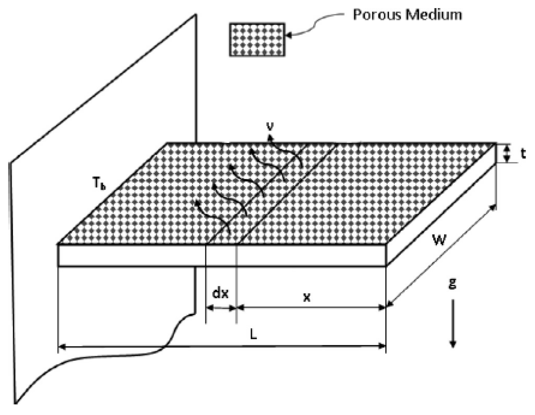
2. Formulation of the Model
When the Temperature Difference in the Fin is Small during Heat Flow
3. Analysis of Nonlinear Heat Transfer Equation Using the Adomian Decomposition Method
Principle of ADM
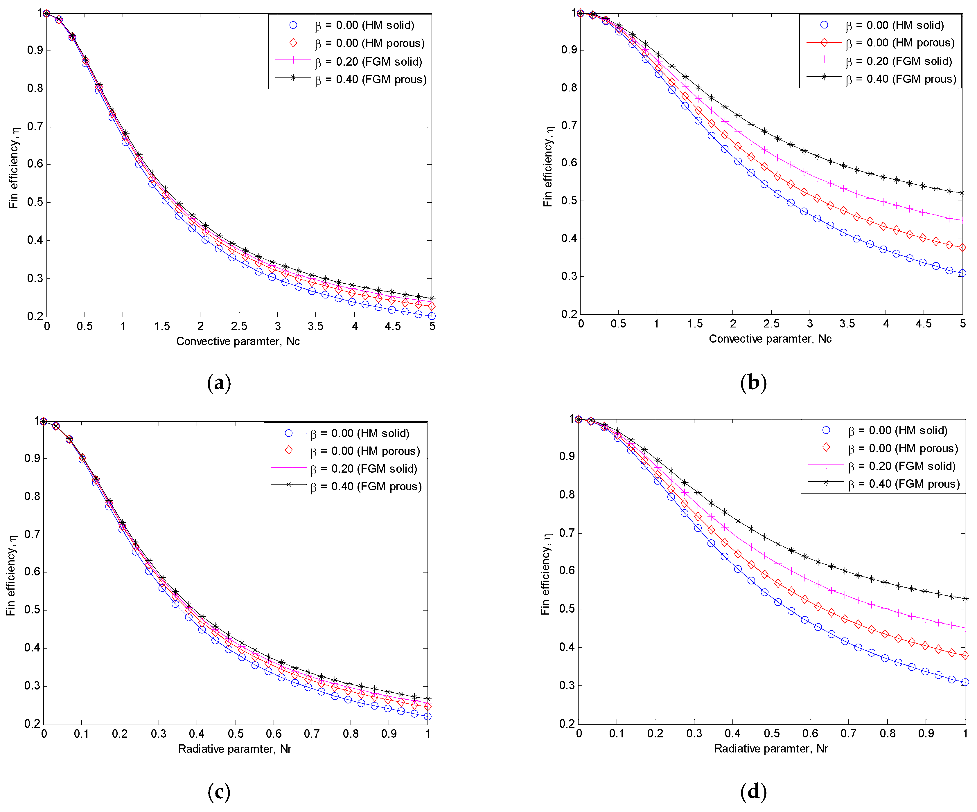
4. Fin Efficiency
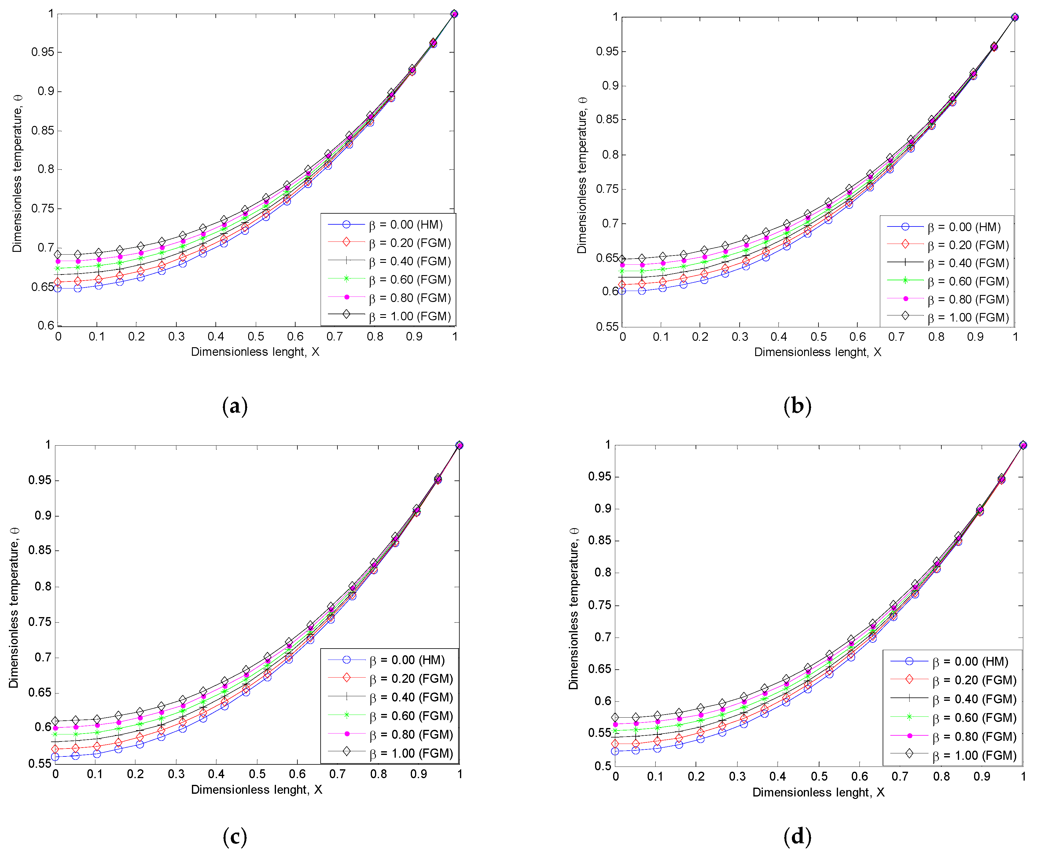
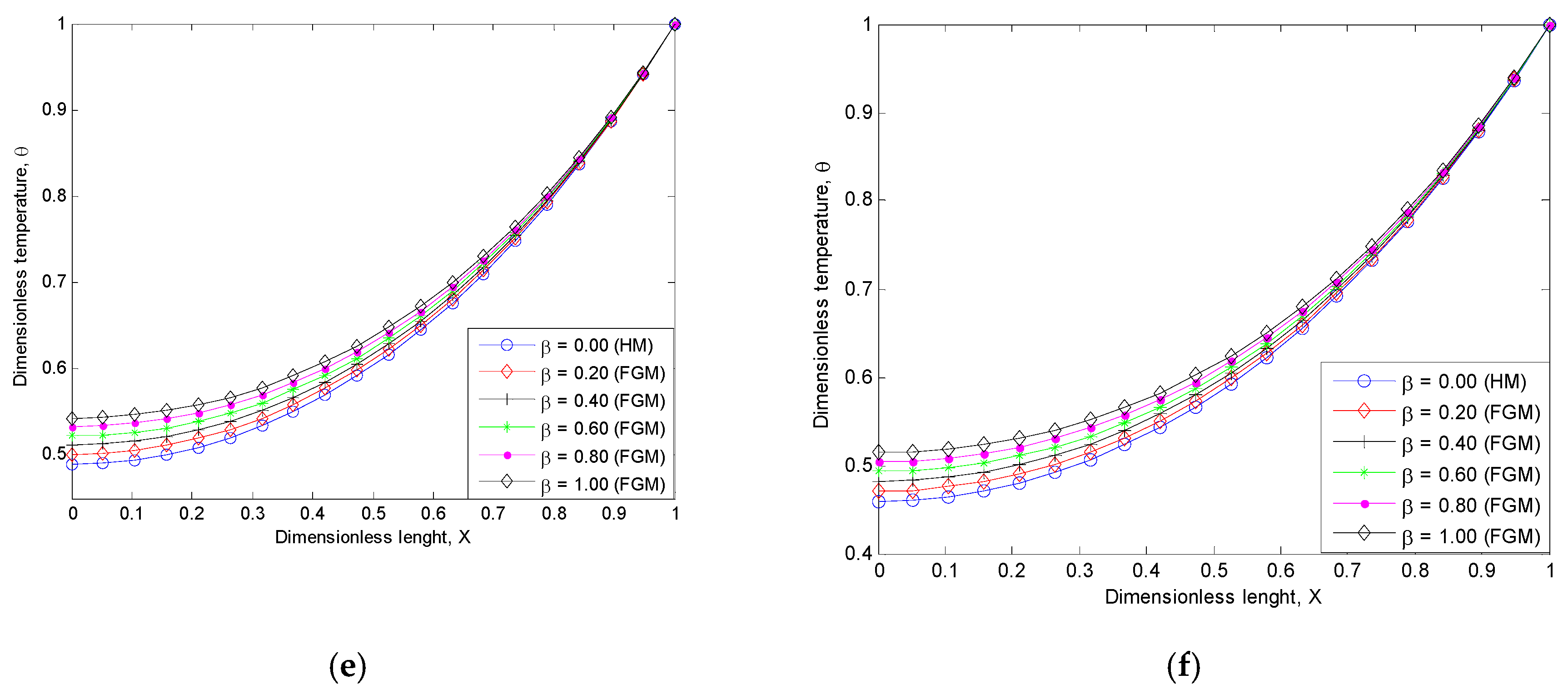
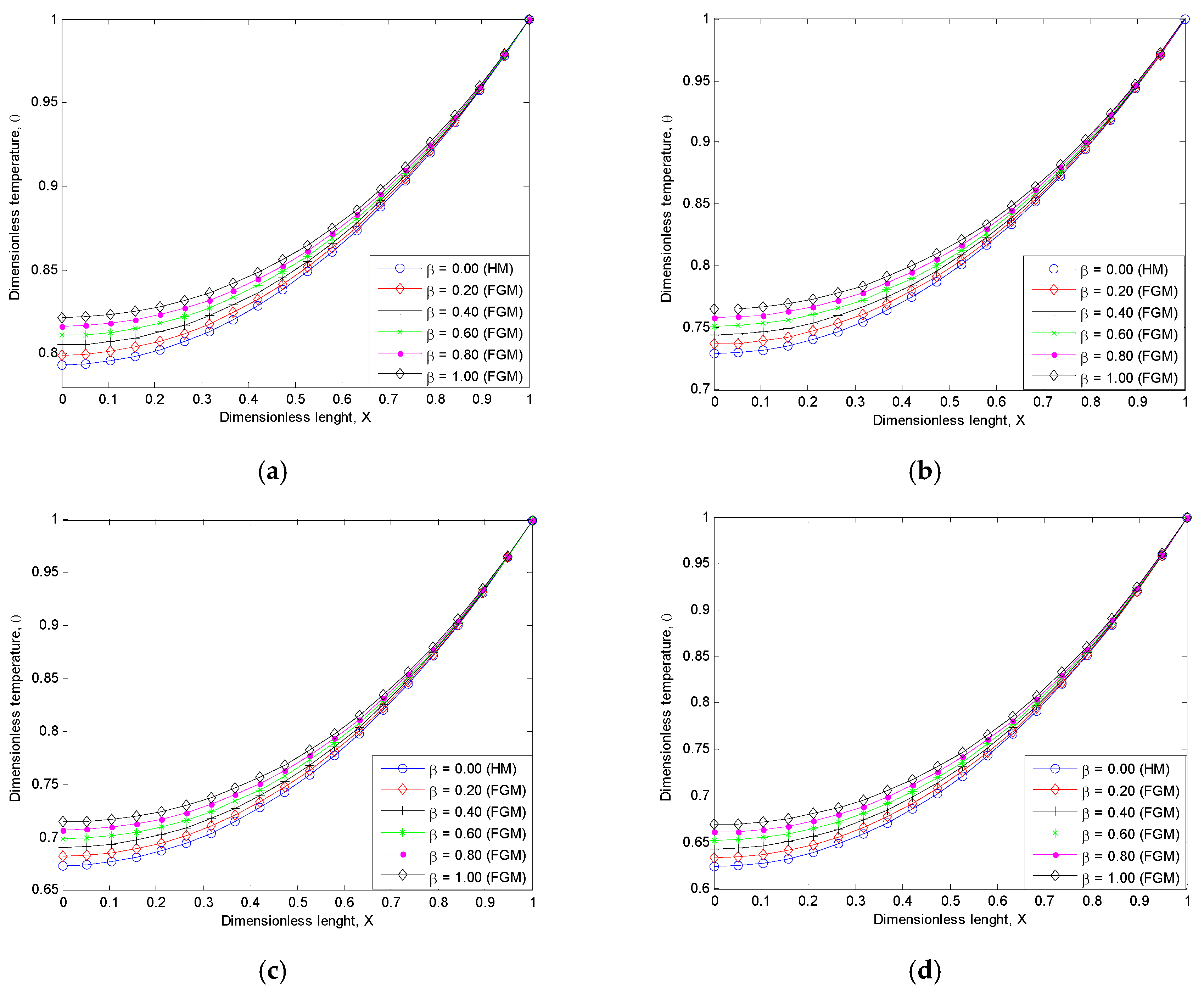
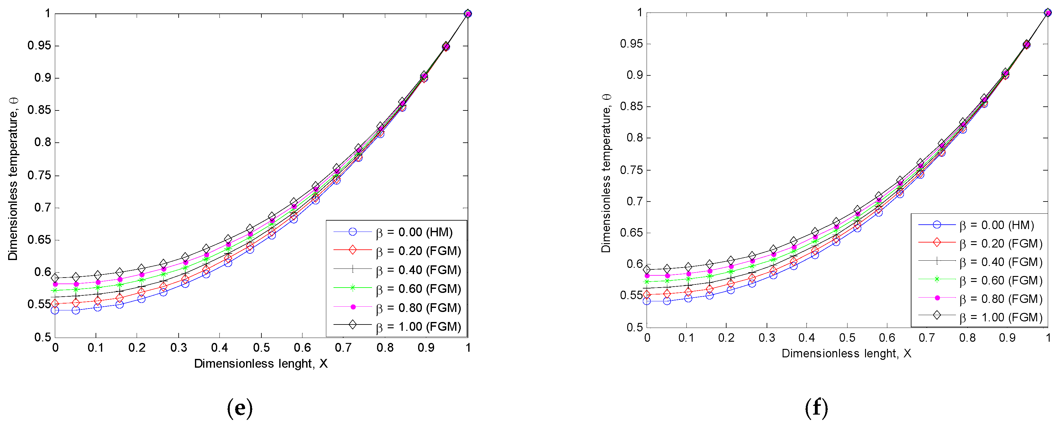
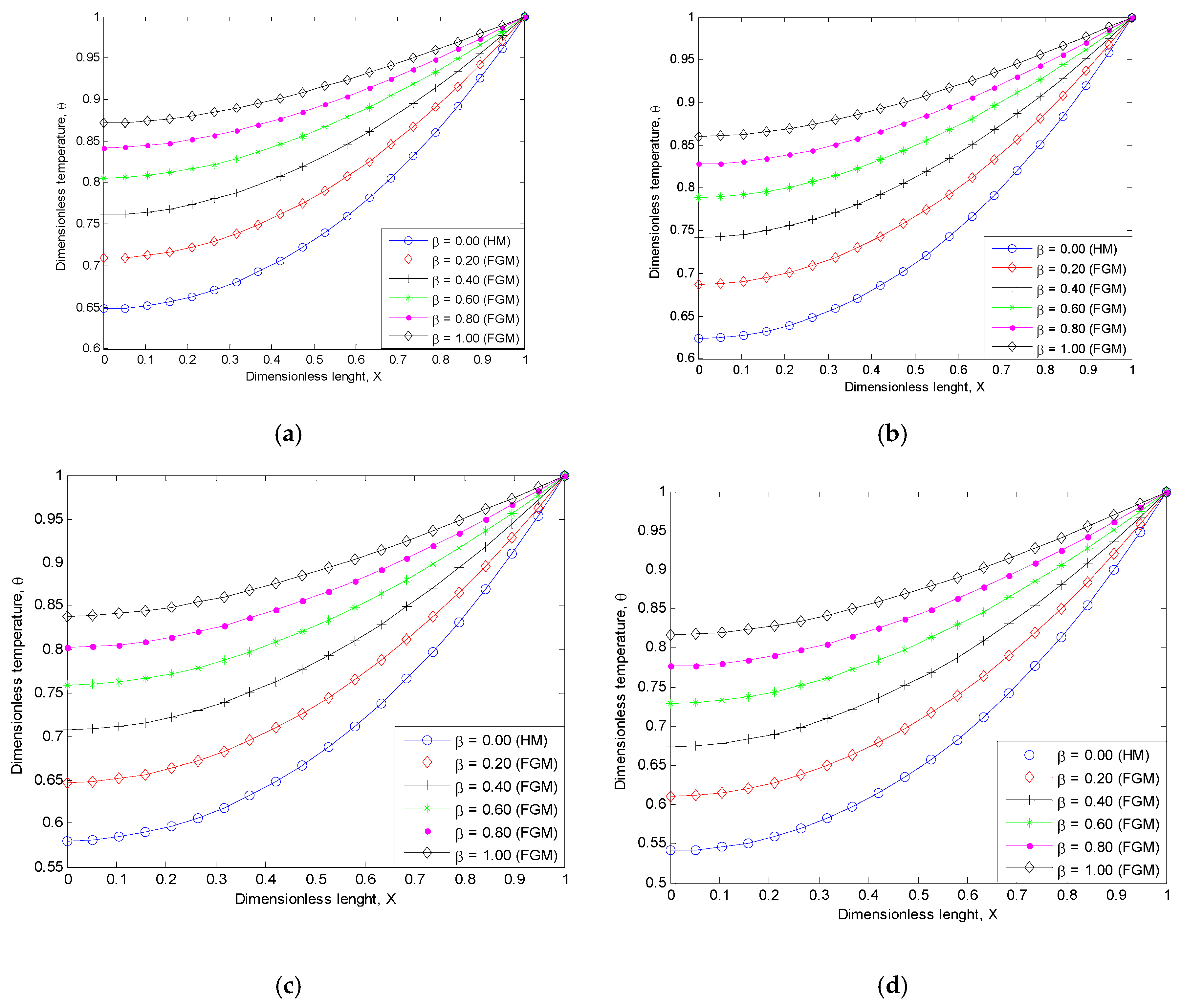
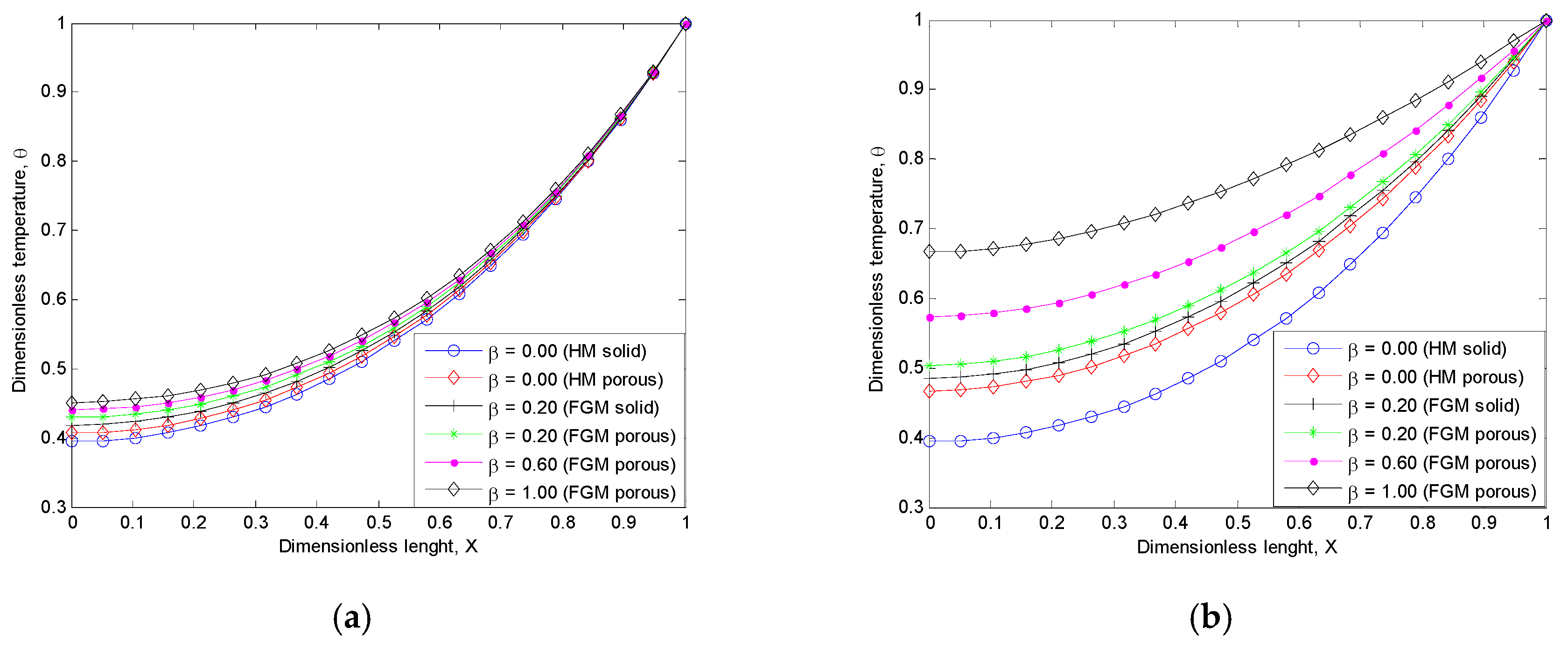
5. Results
6. Conclusions
Author Contributions
Funding
Acknowledgments
Conflicts of Interest
Nomenclature
| A | Fin cross-sectional area, m2 |
| P | Fin perimeter, m |
| hb | Heat transfer coefficient at the base of the fin, Wm−2k−1 |
| cp | Specific heat of the fluid passing through porous fin, J/kg-K |
| h | Heat transfer coefficient over the fin surface, W/m2K |
| H | Dimensionless heat transfer coefficient at fin base, Wm−2k−1 |
| k | Thermal conductivity of fin material, Wm−1k−1 |
| kb | Thermal conductivity of fin material at fin base, Wm−1k−1 |
| keff | Effective thermal conductivity ratio |
| K | Permeability |
| T | Fin temperature, K |
| Tb | Base temperature, K |
| Ta | Ambient temperature, K |
| X | Dimensionless fin length |
| g | Gravity constant m/s2 |
| Da | Darcy number |
| Ra | Rayleigh number |
| Sh | Porosity parameter |
| Nc | Convective heat parameter |
| Nr | Radiative heat parameter |
| M | Dimensionless thermo-geometric parameter |
| Greek Symbols | |
| δ | Fin thickness, m |
| δb | Fin base thickness |
| β | inhomogeneity index |
| θb | Dimensionless temperature at fin base |
| Pores parameter | |
| Porosity or void ratio | |
| η | Fin efficiency |
| ν | kinematic viscosity, m2/s |
| ρ | Density of the fluid, kg/m3 |
| σ | Stefan-Boltzmann constant |
References
- Kiwan, S.; Al-Nimr, M.A. Using Porous Fins for Heat Transfer Enhancement. J. Heat Transf. 2000, 123, 790–795. [Google Scholar] [CrossRef]
- Das, R.; Kundu, B. Prediction of Heat Generation in a Porous Fin from Surface Temperature. J. Thermophys. Heat Transf. 2017, 31, 781–790. [Google Scholar] [CrossRef]
- Oguntala, G.; Sobamowo, G.; Ahmed, Y.; Abd-Alhameed, R. Application of Approximate Analytical Technique Using the Homotopy Perturbation Method to Study the Inclination Effect on the Thermal Behavior of Porous Fin Heat Sink. Math. Comput. Appl. 2018, 23, 62. [Google Scholar] [CrossRef]
- Torabi, M.; Aziz, A.; Zhang, K. A comparative study of longitudinal fins of rectangular, trapezoidal and concave parabolic profiles with multiple nonlinearities. Energy 2013, 51, 243–256. [Google Scholar] [CrossRef]
- Kundu, B.; Das, R.; Wankhade, A.; Lee, K.-S. Heat transfer improvement of a wet fin under transient response with a unique design arrangement aspect. Int. J. Heat Mass Transf. 2018, 127, 1239–1251. [Google Scholar] [CrossRef]
- Kundu, B.; Wongwises, S. A decomposition analysis on convecting–radiating rectangular plate fins for variable thermal conductivity and heat transfer coefficient. J. Frankl. Inst. 2012, 349, 966–984. [Google Scholar] [CrossRef]
- Oguntala, G.; Abd-Alhameed, R. Thermal Analysis of Convective-Radiative Fin with Temperature-Dependent Thermal Conductivity Using Chebychev Spectral Collocation Method. J. Appl. Comput. Mech. 2018, 4, 87–94. [Google Scholar]
- Oguntala, G.; Abd-Alhameed, R.; Sobamowo, G.; Danjuma, I. Performance, Thermal Stability and Optimum Design Analyses of Rectangular Fin with Temperature-Dependent Thermal Properties and Internal Heat Generation. J. Comput. Appl. Mech. 2018, 49, 37–43. [Google Scholar]
- Kundu, B.; Bhanja, D.; Lee, K.-S. A model on the basis of analytics for computing maximum heat transfer in porous fins. Int. J. Heat Mass Transf. 2012, 55, 7611–7622. [Google Scholar] [CrossRef]
- Singh, K.; Das, R.; Kundu, B. Approximate Analytical Method for Porous Stepped Fins with Temperature-Dependent Heat Transfer Parameters. J. Thermophys. Heat Transf. 2016, 30, 661–672. [Google Scholar] [CrossRef]
- Das, R. Forward and inverse solutions of a conductive, convective and radiative cylindrical porous fin. Energy Convers. Manag. 2014, 87, 96–106. [Google Scholar] [CrossRef]
- Oguntala, G.; Sobamowo, G.; Abd-Alhameed, R.; Jones, S. Efficient Iterative Method for Investigation of Convective–Radiative Porous Fin with Internal Heat Generation Under a Uniform Magnetic Field. Int. J. Appl. Comput. Math. 2019, 5, 13. [Google Scholar] [CrossRef]
- Oguntala, G.A.; Sobamowo, M.G. Galerkin’s Method of Weighted Residual for a Convective Straight Fin with Temperature-Dependent Conductivity and Internal Heat Generation. Int. J. Eng. Technol. 2016, 6, 432–442. [Google Scholar]
- Oguntala, G.; Sobamowo, G.; Abd-Alhameed, R. Numerical analysis of transient response of convective-radiative cooling fin with convective tip under magnetic field for reliable thermal management of electronic systems. Therm. Sci. Eng. Prog. 2019, 9, 289–298. [Google Scholar] [CrossRef]
- Oguntala, G.A.; Abd-Alhameed, R.A. Haar Wavelet Collocation Method for Thermal Analysis of Porous Fin with Temperature-dependent Thermal Conductivity and Internal Heat Generation. J. Appl. Comput. Mech. 2017, 3, 185–191. [Google Scholar]
- Das, R.; Kundu, B. Direct and inverse approaches for analysis and optimization of fins under sensible and latent heat load. Int. J. Heat Mass Transf. 2018, 124, 331–343. [Google Scholar] [CrossRef]
- Seyf, H.R.; Feizbakhshi, M. Computational analysis of nanofluid effects on convective heat transfer enhancement of micro-pin-fin heat sinks. Int. J. Therm. Sci. 2012, 58, 168–179. [Google Scholar] [CrossRef]
- Fazeli, S.A.; Hashemi, H.; Mohammad, S.; Zirakzadeh, H.; Ashjaee, M. Experimental and numerical investigation of heat transfer in a miniature heat sink utilizing silica nanofluid. Superlattices Microstruct. 2012, 51, 247–264. [Google Scholar] [CrossRef]
- Kim, S.-M.; Mudawar, I. Analytical heat diffusion models for different micro-channel heat sink cross-sectional geometries. Int. J. Heat Mass Transf. 2010, 53, 4002–4016. [Google Scholar] [CrossRef]
- Naphon, P.; Klangchart, S.; Wongwises, S. Numerical investigation on the heat transfer and flow in the mini-fin heat sink for CPU. Int. Commun. Heat Mass Transf. 2009, 36, 834–840. [Google Scholar] [CrossRef]
- Naphon, P.; Khonseur, O. Study on the convective heat transfer and pressure drop in the micro-channel heat sink. Int. Commun. Heat Mass Transf. 2009, 36, 39–44. [Google Scholar] [CrossRef]
- Kim, T.Y.; Kim, S.J. Fluid flow and heat transfer characteristics of cross-cut heat sinks. Int. J. Heat Mass Transf. 2009, 52, 5358–5370. [Google Scholar] [CrossRef]
- Oguntala, G.A.; Abd-Alhameed, R.A.; Sobamowo, G.M.; Eya, N. Effects of particles deposition on thermal performance of a convective-radiative heat sink porous fin of an electronic component. Therm. Sci. Eng. Prog. 2018, 6, 177–185. [Google Scholar] [CrossRef]
- Oguntala, G.; Abd-Alhameed, R. Performance of convective-radiative porous fin heat sink under the influence of particle deposition and adhesion for thermal enhancement of electronic components. Karbala Int. J. Mod. Sci. 2018, 4, 297–312. [Google Scholar] [CrossRef]
- Oguntala, G.A.; Sobamowo, G.M.; Eya, N.N.; Abd-Alhameed, R.A. Investigation of Simultaneous Effects of Surface Roughness, Porosity, and Magnetic Field of Rough Porous Microfin Under a Convective–Radiative Heat Transfer for Improved Microprocessor Cooling of Consumer Electronics. IEEE Trans. Compon. Packag. Manuf. Technol. 2019, 9, 235–246. [Google Scholar] [CrossRef]
- Wan, Z.M.; Guo, G.Q.; Su, K.L.; Tu, Z.K.; Liu, W. Experimental analysis of flow and heat transfer in a miniature porous heat sink for high heat flux application. Int. J. Heat Mass Transf. 2012, 55, 4437–4441. [Google Scholar] [CrossRef]
- Oguntala, G.; Abd-Alhameed, R.; Sobamowo, G. On the effect of magnetic field on thermal performance of convective-radiative fin with temperature-dependent thermal conductivity. Karbala Int. J. Mod. Sci. 2018, 4, 1–11. [Google Scholar] [CrossRef]
- Sobamowo, M.G.; Oguntala, G.A.; Yinusa, A.A. Nonlinear Transient Thermal Modeling and Analysis of a Convective-Radiative Fin with Functionally Graded Material in a Magnetic Environment. Model. Simul. Eng. 2019, 2019, 7878564. [Google Scholar] [CrossRef]
- Sobamowo, M.G.; Kamiyo, O.M.; Adeleye, O.A. Thermal performance analysis of a natural convection porous fin with temperature-dependent thermal conductivity and internal heat generation. Therm. Sci. Eng. Prog. 2017, 1, 39–52. [Google Scholar] [CrossRef]


| X | Numerical Method (NM) | Homotopy Perturbation Method (HPM) [29] | Galerkin’s Method of Weighted Residual (GMWR) [29] | Adomian Decomposition Method (ADM) (Present Study) | Absolute Error in HPM (NM-HPM) | Absolute Error in GMWR (NM-HPM) | Absolute Error in ADM (NM-HPM) |
|---|---|---|---|---|---|---|---|
| 0.0 | 0.9581 | 0.9581 | 0.9581 | 0.9581 | 0.0000 | 0.0000 | 0.0000 |
| 0.1 | 0.9585 | 0.9585 | 0.9585 | 0.9585 | 0.0000 | 0.0000 | 0.0000 |
| 0.2 | 0.9597 | 0.9597 | 0.9597 | 0.9597 | 0.0000 | 0.0000 | 0.0000 |
| 0.3 | 0.9618 | 0.9618 | 0.9618 | 0.9618 | 0.0000 | 0.0000 | 0.0000 |
| 0.4 | 0.9647 | 0.9647 | 0.9647 | 0.9647 | 0.0000 | 0.0000 | 0.0000 |
| 0.5 | 0.9685 | 0.9685 | 0.9685 | 0.9685 | 0.0000 | 0.0000 | 0.0000 |
| 0.6 | 0.9730 | 0.9730 | 0.9730 | 0.9730 | 0.0000 | 0.0000 | 0.0000 |
| 0.7 | 0.9785 | 0.9785 | 0.9785 | 0.9785 | 0.0000 | 0.0000 | 0.0000 |
| 0.8 | 0.9846 | 0.9846 | 0.9846 | 0.9846 | 0.0000 | 0.0000 | 0.0000 |
| 0.9 | 0.9919 | 0.9919 | 0.9919 | 0.9919 | 0.0000 | 0.0000 | 0.0000 |
| 1.0 | 1.0000 | 1.0000 | 1.0000 | 1.0000 | 0.0000 | 0.0000 | 0.0000 |
© 2019 by the authors. Licensee MDPI, Basel, Switzerland. This article is an open access article distributed under the terms and conditions of the Creative Commons Attribution (CC BY) license (http://creativecommons.org/licenses/by/4.0/).
Share and Cite
Oguntala, G.; Sobamowo, G.; Ahmed, Y.; Abd-Alhameed, R. Thermal Prediction of Convective-Radiative Porous Fin Heatsink of Functionally Graded Material Using Adomian Decomposition Method. Computation 2019, 7, 19. https://0-doi-org.brum.beds.ac.uk/10.3390/computation7010019
Oguntala G, Sobamowo G, Ahmed Y, Abd-Alhameed R. Thermal Prediction of Convective-Radiative Porous Fin Heatsink of Functionally Graded Material Using Adomian Decomposition Method. Computation. 2019; 7(1):19. https://0-doi-org.brum.beds.ac.uk/10.3390/computation7010019
Chicago/Turabian StyleOguntala, George, Gbeminiyi Sobamowo, Yinusa Ahmed, and Raed Abd-Alhameed. 2019. "Thermal Prediction of Convective-Radiative Porous Fin Heatsink of Functionally Graded Material Using Adomian Decomposition Method" Computation 7, no. 1: 19. https://0-doi-org.brum.beds.ac.uk/10.3390/computation7010019