Spatiotemporal Dynamics of a Generalized Viral Infection Model with Distributed Delays and CTL Immune Response


1
Centre Régional des Métiers de l’Education et de la Formation (CRMEF), 20340 Derb Ghalef, Casablanca, Morocco
2
Laboratory of Analysis, Modeling and Simulation (LAMS), Faculty of Sciences Ben M’sik, Hassan II University, P.O. Box 7955, Sidi Othman, Casablanca, Morocco
Computation 2019, 7(2), 21; https://0-doi-org.brum.beds.ac.uk/10.3390/computation7020021
Submission received: 13 February 2019
/
Revised: 29 March 2019
/
Accepted: 4 April 2019
/
Published: 15 April 2019
(This article belongs to the Section Computational Biology)
Abstract
:In this paper, we propose and investigate a diffusive viral infection model with distributed delays and cytotoxic T lymphocyte (CTL) immune response. Also, both routes of infection that are virus-to-cell infection and cell-to-cell transmission are modeled by two general nonlinear incidence functions. The well-posedness of the proposed model is also proved by establishing the global existence, uniqueness, nonnegativity and boundedness of solutions. Moreover, the threshold parameters and the global asymptotic stability of equilibria are obtained. Furthermore, diffusive and delayed virus dynamics models presented in many previous studies are improved and generalized.
1. Introduction
During human infections with viruses such as human immunodeficiency virus (HIV), human T-cell leukemia virus (HTLV), hepatitis B virus (HBV) and hepatitis C virus (HCV), cytotoxic T lymphocyte (CTL) cells play a crucial role in antiviral defence by attacking and killing infected cells. So, modeling the role of CTL immune response in viral infection has attracted the attention of many researchers. In 1996, Nowak and Bangham [1] proposed a basic mathematical model by assuming that the infection process is bilinear and follows the principle of mass action. However, as a nonlinear relationship between parasite dose and infection rate has been frequently observed in experiments in [2,3], this bilinear incidence was replaced by Beddington-DeAngelis functional response in [4] and by a more general incidence function in [5].
In the above classical models that are formulated by ordinary differential equations (ODEs), the cell infection is instantaneous and only caused by contact with the free virus. In reality, there are two routes of infection and also time delays in cell infection and virus production. Motivated by these biological reasons, Li et al. [6] proposed a mathematical model formulated by delay differential equations (DDEs) to describe the global dynamics of HIV infection with CTL immune response. This delayed model is an extension of [1] that considers Holling type-II functional response and two kinds of discrete delays, one in cell infection and the other in virus production. Also, the authors of [7] improved the model of Nowak and Bangham [1] by introducing a discrete delay in cell infection and using a Crowley-Martin type incidence function. In 2016, Wang et al. [8] introduced an infinite distributed delay in cell infection in order to improve the basic model with CTL immune response [1], and they also considered both routes of infection, virus-to-cell infection and cell-to-cell transmission. Furthermore, a recent work presented in [9] studied the dynamical behavior of a viral infection model with two types of distributed time delays, CTL immune response and saturated incidence rates for both routes of infection. In this paper, we generalize all the ODE and DDE models presented in [1,4,5,6,7,8,9] by proposing the following nonlinear system:
where , , and denote the densities of susceptible target cells, infected target cells, free virus particles and CTL cells at time t, respectively. The susceptible target cells are produced at constant , die at rate d and become infected by contact with free virus at rate and by contact with infected cells at rate . The parameters a and b are the death rates of infected cells and CTL cells. The parameter p represents the rate at which infected cells are killed by CTL cells, k is the production rate of free virus by an infected cell, and is the clearance rate of free virus. CTL cells expand in response to viral antigens derived from infected cells at rate cIZ. Further, we assume that the virus or infected cell contacts an uninfected cell at time and the cell becomes infected at time t, where is a random variable taken from a probability distribution . The term represents the probability of surviving from time to time t, where is the death rate for infected but not yet virus-producing cells. In the same, we assume that the time necessary for the newly produced virions to become mature and infectious is a random variable with a probability distribution . The term denotes the probability of the immature virions surviving the delay period, where is the average life time of an immature virus. Therefore, the integral describes the mature viral particles produced at time t. The probability distribution functions and are assumed to satisfy and for .
As in [10,11], the incidence functions and for both routes of infection are continuously differentiable and satisfy the following hypotheses:
- (H0)
- g(0,I) = 0, for all ; (or is a strictly monotone increasing function with respect to T when ) and , for all and .
- (H1)
- , for all and ,
- (H2)
- is a strictly monotone increasing function with respect to T (or when is a strictly monotone increasing function with respect to T), for any fixed and ,
- (H3)
- is a monotone decreasing function with respect to I and V.
From a biological viewpoint, the above hypotheses are reasonable and consistent with reality. In fact, the first assumption () on the function means that the incidence rate by direct contact with infected cells is equal to zero if there are no susceptible cells. This incidence rate is increasing when the number of infected cells is constant and the number of susceptible cells increases. Also, it is decreasing when the number of susceptible cells is constant and the number of infected cells increases. Similarly, the second assumption () on the function means that the incidence rate by contact with free virus is equal to zero if there are no susceptible cells. By () and (), this incidence rate is increasing when the numbers of infected cells and virus are constant and the number of susceptible cells increases. Also, it is decreasing when the number of susceptible is constant and the number of infected cells or free virus increases. Consequently, the more susceptible cells are, the more infectious events will occur. However, the higher the number of infected cells or the concentration of virus in the host is, the less infectious events will be [10,12,13]. In addition, the functions and cover several types of incidence rates existing in the literature such as the classical bilinear incidence, standard incidence, Holling type-II functional response, Beddington-DeAngelis functional response, Crowley-Martin functional response and Hattaf-Yousfi functional response.
On the other hand, system (1) assumes that cells and viruses are well mixed, and ignores their mobility. Actually, viral propagation is a localized process [14] due to the fact that the virus is inherently unstable and the infection occurs mainly in lymphoid tissues. Also, the interaction between virus and the immune response tends to be local within the body of infected hosts [15]. Further, cells are distributed in space and typically interact with the physical environment and other organisms in their spatial neighborhood [16]. Therefore, it is more reasonable to study a reaction-diffusion version of system (1). So, the organization of this paper is as follows. In the next section, we present the reaction-diffusion version of (1) and some preliminary results. Section 3 is devoted to the global dynamics of the reaction-diffusion model. An application and some numerical simulations of our main results are presented in Section 4. Finally, the paper ends with mathematical and biological conclusions in the last section.
2. Model Formulation and Preliminaries
We first present a reaction-diffusion version of system (1) by taking into account the mobility of cells and viruses. Hence, system (1) becomes
where , , and are the densities of susceptible target cells, infected target cells, free virus particles and CTL cells at location x and time t, respectively. Here, we assume that the motion of the above four populations follows Fickian diffusion, meaning that the fluxes of these four populations are proportional to their concentration gradient and go from regions of high concentration to regions of low concentration, with the diffusion coefficients , , and , respectively. △ is the Laplacian operator. The other parameters have the same biological meanings as those in system (1).
It is very important to note that our model (2) formulated by partial differential equations (PDEs) extends and generalizes many virus dynamics models existing in the literature. For instance, we obtain the diffused HBV infection model proposed by Wang et al. [17] when , , and , where , is a constant rate describing the infection process and is the Dirac delta function. When , , , and , where are constants, we get the diffusive and delayed viral infection model with Beddington-DeAngelis functional response [18]. Also, the diffusive and delayed viral infection model with Crowley-Martin functional response [19] is a special case of (2), it suffices to take , , , and .
Throughout this paper, we consider system (2) with initial conditions
and zero-flux boundary conditions
where is a bounded domain in with smooth boundary , and indicates the outward normal derivative on . From the biological point of view, these conditions mean that the uninfected cells, infected cells, free virus particles and CTL cells do not move across the boundary .
We now study the well posedness of the PDE model (2) by establishing the global existence, uniqueness, nonnegativity and boundedness of solutions. To this end, we need some notations. Let be the Banach space of continuous functions from into , and be the Banach space of continuous functions from into , where is uniformly continuous on and with is a positive constant. For convenience, we identify an element as a function from into defined by . For any continuous function : for , we define by , . It is not hard to prove that is a continuous function from to . Moreover, we need the following lemma.
Lemma 1.
Let A, B and D be three constants with . Consider the following problem
Then. Moreover, if, we have
Proof.
Let be a solution to the ordinary differential equation
Then . It follows from the comparison principle [20] that . Hence,
So, if , we have and
☐
Theorem 1.
Proof.
Let and . We define by
Then problem (2)–(4) can be rewritten as the following abstract functional differential equation
where , and . It is obvious that F is locally Lipschitz in . According to [21,22,23,24,25], we deduce that system (6) admits a unique local solution on its maximal interval of existence .
From the first equation of (2), we get
By Lemma 1, we get
This implies that T is bounded. Let
The integral in is well-defined and differentiable with respect to t, due to T being bounded. Thus,
where and
When , we have
From Lemma 1, we have
Thus, I and Z are bounded. It remains to prove that V is bounded. From the boundedness of I and (2)–(4), we deduce that V satisfies the following system
where . According to Lemma 1, we deduce that
This implies that V is bounded. From the above, we have proved that , , and are bounded on . By the standard theory for semilinear parabolic systems [26], we deduce that . This completes the proof. ☐
Clearly, system (2) has always one infection-free equilibrium , where , which represents the healthy state. Hence, we define the basic reproduction number for our PDE model as follows
Biologically and as in [11,27], can be divided into parts as , where is the basic reproduction number corresponding to virus-to-cell infection mode, and is the basic reproduction number corresponding to cell-to-cell transmission mode.
The other spatially uniform steady states of (2) satisfy the following system
The last equation of (12) implies that or . Hence, we discuss two cases.
For the case when , we get
Since , we have . Then there is no biological equilibrium whenever . Let us define the function on the interval by
It follows from ()–() that , and
which implies that there exists a unique such as provided that . Thus, is a unique infection equilibrium of (2) with and .
For the case when , we have , and
Since , we have . Then there is no positive equilibrium when or . Define the function on the interval by
If CTL immune response has not been established, we have . So, we define the reproduction number for cellular immunity as follows
where denotes the average life expectancy of CTL cells and is the number of infected cells at . Hence, represents the average number of the CTL immune cells activated by infected cells.
If , then , and
So, there is no equilibrium when .
If , then , and Hence, if , system (2) has a CTL-activated infection equilibrium , where , , and .
Recapitulating the above discussions in the following theorem.
3. Global Stability
Regarding the global stability of the infection-free equilibrium , we have the following theorem.
Theorem 3.
The infection-free equilibriumof system (2) is globally asymptotically stable when.
Proof.
Based on the method proposed in [28], we construct the Lyapunov functional for system (2) at as follows
For convenience, we let and for any . The time derivative of along the solution of system (2) satisfies
From (7) and by applying Lemma 1, we get . This implies that all omega limit points satisfy . Hence, it is sufficient to consider solutions for which . From the explicit formula of given in (11) and -, we get
Hence, ensures . In addition, it can be shown that the largest compact invariant set in is the singleton . Therefore, it follows from LaSalle’s invariance principle [29] that is globally asymptotically stable when . ☐
For the global stability of the two infection steady states of system (2), we suppose that and the incidence functions f and g satisfy for each infection equilibrium the following further hypothesis
Therefore, we have the following result.
Theorem 4.
Assumeand (H4) holds for each.
Proof.
For (i), we construct the Lyapunov functional as follows
where , . Clearly, attains its strict global minimum at and . Then and so the functional is non-negative.
Calculating the time derivative of along the solution of system (2), we obtain
Using and , we get
Since the function is strictly monotonically increasing with respect to T, we have for that
Since and , we have with equality if and only if , , and . It follows from LaSalle’s invariance principle that is globally asymptotically stable.
For (ii), we construct the Lyapunov functional as follows
Calculating the time derivative of along the solution of system (2) and using , and , we have
Remark 1.
The hypothesis (H4) comes from (17) and (18). This hypothesis is a sufficient condition for that the time derivatives of the Lyapunov functionalsandto be non-negative. When cell-to-cell mode is ignored (i.e.,), the assumption (H4) can be reduced to
which is verified by many types of the incidence rate including the bilinear incidence, the saturation incidence, the Beddington-DeAnglis functional response, the Crowley-Martin functional response and the Hattaf-Yousfi functional response.
In 2017, Xu et al. [30] proposed a PDE model with two discrete delays, cell-to-cell transmission and CTL immune response. They considered the spatial diffusion only in virus. This model is given by
where the functions and satisfy the following properties:
Choose the functions and as follows
4. Application and Numerical Simulations
In this section, we first apply our main results obtained in this study to the following model:
where and denote, respectively, the virus-to-cell infection rate and the cell-to-cell transmission rate. The non-negative constants and measure the saturation effect. The other state variables and parameters have the same biological meanings as in models (1) and (2). Notice that system (21) extends the DDE model presented in [9] by introducing the spacial diffusion in both cells and viruses. Also, this system is a particular case of (2) with and . As before, we consider system (21) with initial conditions
and Neumann boundary conditions
It is easy to check the first four hypotheses -. For the fifth hypothesis, we have
Thus, the last hypothesis (H4) is verified. By applying Theorems 3 and 4, we obtain the following result.
Corollary 1.
- If, then system (21) has two infection equilibria that are:
- (i)
- the infection equilibrium without cellular immunitythat is globally asymptotically stable if;
- (ii)
- the infection equilibrium with cellular immunitythat is globally asymptotically stable if.
For the numerical simulations, we choose for . Clearly, . Also, we consider the following new variables:
Then the variables T, Y, I, U, V and Z satisfy the following system:
The threshold parameters and for (24) are given by (11) and (15) with and . For the simplicity of numerical illustrations, we consider one-dimensional bounded spatial domain with and . Also, we consider and c as free parameters. All other parameter values are mentioned in Table 1.
When and , we have . By the first result given in Corollary 1, the infection-free equilibrium is globally asymptotically stable. This means that the virus is cleared, the infection dies out and the patient will be completely cured (see Figure 1).
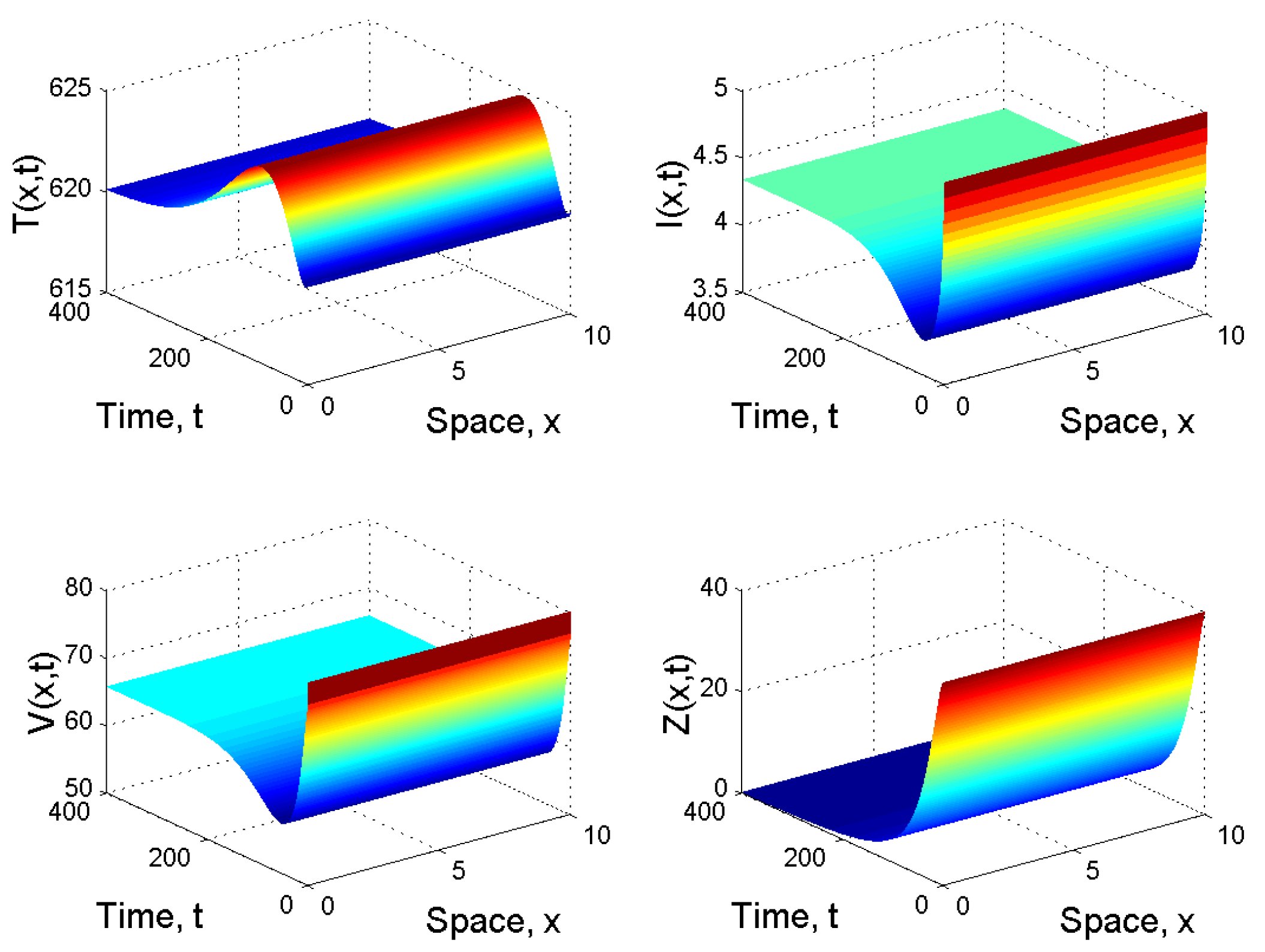
When and , we obtained and . From Corollary 1 2(i), we know that is globally asymptotically stable (see Figure 2).
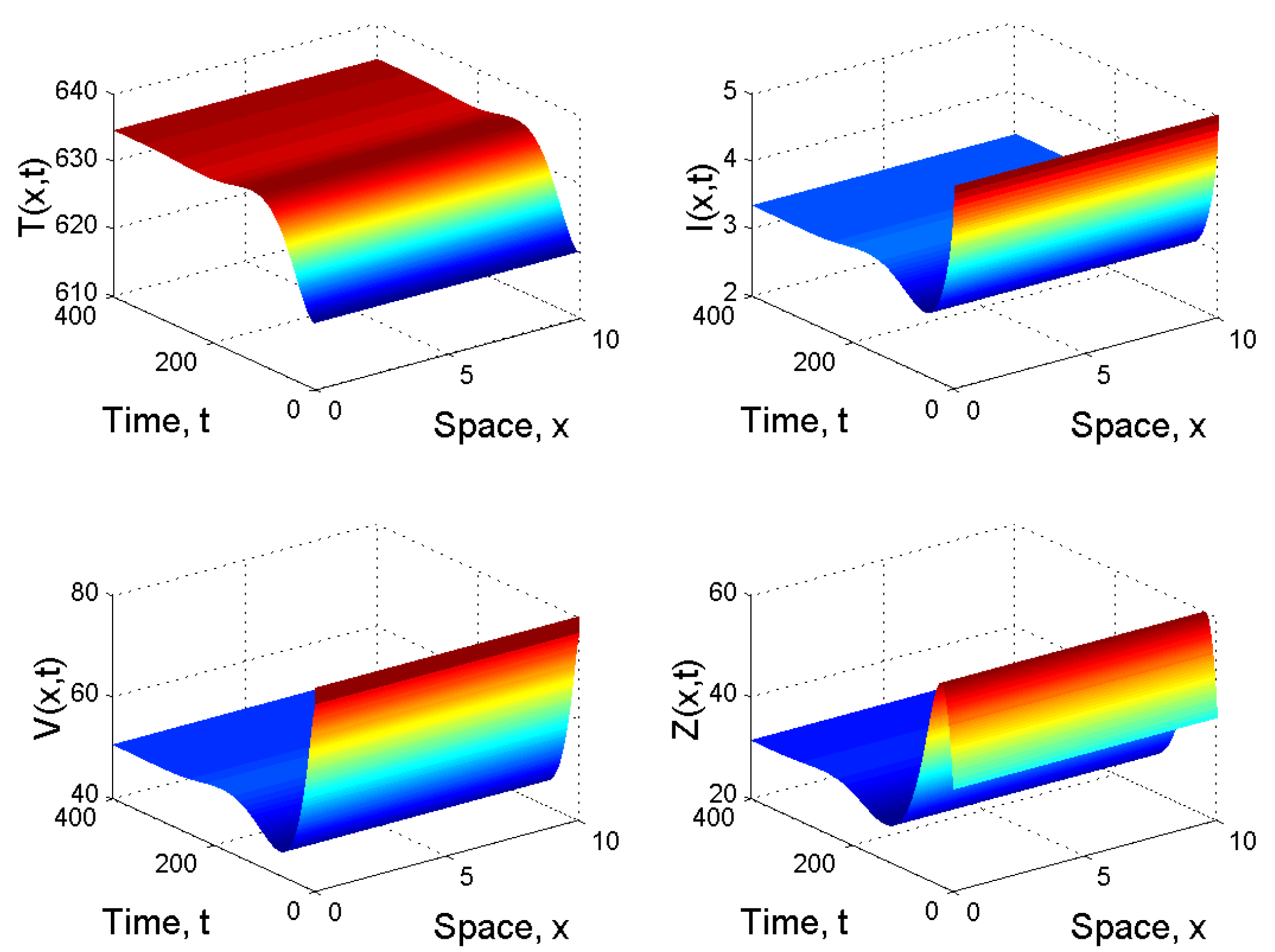
When and , we obtained and . It follows from Corollary 1 2(ii) that is globally asymptotically stable (see Figure 3).
5. Conclusions
In this article, we have proposed and investigated a generalized viral infection model with two infinite distributed delays, CTL immune response and spatial diffusion in both cells and virus. Also, the proposed model incorporated the classical virus-to-cell infection and the direct cell-to-cell transmission. Both routes of infection are modeled by two general incidence functions. Under some assumptions on these incidence functions, we have shown that the global dynamics of the model is completely determined by two threshold parameters that are the basic reproduction number and the reproduction numbers for cellular immunity . From the viewpoint of biology, we have proved that when the infection-free equilibrium is globally asymptotically stable, which means that the virus is cleared and the infection dies out. Whereas, the virus persists in the host if and two steady states appear, one without cellular immunity which is globally asymptotically stable if and the other with cellular immunity which is globally asymptotically stable if . Hence, the activation of the CTL immune response is unable to eliminate the virus in vivo, but plays a fundamental role in the reduction of virus particles and infected cells. This last biological result can be easily deduced by comparing the components of virus particles and infected cells before and after the activation of cellular immunity. Since and have no relation to the diffusion coefficients , , and , we conclude that the diffusion of cells and virus has no effect on the global stability of the three steady states of our PDE model with Neumann homogeneous boundary conditions. On the other hand, we have extended the models with ODEs [1,4,5], with DDEs [6,7,8,9] and with PDEs [17,18,19]. Moreover, the more recent works presented in [30,31] are improved and generalized.
Funding
This research received no external funding.
Acknowledgments
The author would like to express his sincere thanks to the editor and anonymous reviewers for their helpful comments and valuable suggestions which significantly improved the quality of this paper.
Conflicts of Interest
The author declares no conflict of interest.
References
- Nowak, M.A.; Bangham, C.R.M. Population dynamics of immune responses to persistent viruses. Science 1996, 272, 74–79. [Google Scholar] [CrossRef]
- Ebert, D.; Zschokke-Rohringer, C.D.; Carius, H.J. Dose effects and density-dependent regulation of two microparasites of Daphnia magna. Oecologia 2000, 122, 200–209. [Google Scholar] [CrossRef] [PubMed]
- Mclean, A.R.; Bostock, C.J. Scrapie infections initiated at varying doses: An analysis of 117 titration experiments. Philos. Trans. Roy. Soc. London Ser. B 2000, 355, 1043–1050. [Google Scholar] [CrossRef] [PubMed]
- Wang, X.; Tao, Y.; Song, X. Global stability of a virus dynamics model with Beddington-DeAngelis incidence rate and CTL immune response. Nonlinear Dyn. 2011, 66, 825–830. [Google Scholar] [CrossRef]
- Hattaf, K.; Yousfi, N.; Tridane, A. Global stability analysis of a generalized virus dynamics model with the immune response. Can. Appl. Math. Q. 2012, 20, 499–518. [Google Scholar]
- Li, Y.; Xu, R.; Li, Z.; Mao, S. Global dynamics of a delayed HIV-1 infection model with CTL immune response. Discret. Dyn. Nat. Soc. 2011, 2011, 673843. [Google Scholar] [CrossRef]
- Li, X.; Fu, S. Global stability of a virus dynamics model with intracellular delay and CTL immune response. Math. Methods Appl. Sci. 2015, 38, 420–430. [Google Scholar] [CrossRef]
- Wang, J.; Guo, M.; Liu, X.; Zhao, Z. Threshold dynamics of HIV-1 virus model with cell-to-cell transmission, cell-mediated immune responses and distributed delay. Appl. Math. Comput. 2016, 291, 149–161. [Google Scholar] [CrossRef]
- Elaiw, A.M.; Raezah, A.A.; Hattaf, K. Stability of HIV-1 infection with saturated virus-target and infected-target incidences and CTL immune response. Int. J. Biomath. 2017, 10, 1–29. [Google Scholar] [CrossRef]
- Hattaf, K.; Yousfi, N. A generalized virus dynamics model with cell-to-cell transmission and cure rate. Adv. Differ. Equ. 2016, 2016, 174. [Google Scholar] [CrossRef]
- Hattaf, K.; Yousfi, N. Qualitative analysis of a generalized virus dynamics model with both modes of transmission and distributed delays. Int. J. Differ. Equ. 2018, 2018, 9818372. [Google Scholar] [CrossRef]
- Hattaf, K.; Yousfi, N. A numerical method for a delayed viral infection model with general incidence rate. J. King Saud Univ.-Sci. 2016, 28, 368–374. [Google Scholar] [CrossRef] [Green Version]
- Wang, X.-Y.; Hattaf, K.; Huo, H.-F.; Xiang, H. Stability analysis of a delayed social epidemics model with general contact rate and its optimal control. J. Ind. Manag. Optim. 2016, 12, 1267–1285. [Google Scholar] [CrossRef] [Green Version]
- Strain, M.C.; Richman, D.D.; Wong, J.K.; Levine, H. Spatiotemporal dynamics of HIV propagation. J. Theor. Biol. 2002, 218, 85–96. [Google Scholar] [CrossRef]
- Funk, G.A.; Jansen, V.A.; Bonhoeffer, S.; Killingback, T. Spatial models of virus-immune dynamics. J. Theor. Biol. 2005, 233, 221–236. [Google Scholar] [CrossRef] [PubMed]
- Cantrell, R.; Cosner, C. Spatial Ecology via Reaction Diffusion Equations; Wiley: New York, NY, USA, 2003. [Google Scholar]
- Wang, S.; Feng, X.; He, Y. Global asymptotical properties for a diffused HBV infection model with CTL immune response and nonlinear incidence. Acta Math. Sci. 2011, 31, 1959–1967. [Google Scholar]
- Yang, Y.; Xu, Y. Global stability of a diffusive and delayed virus dynamics model with Beddington-DeAngelis incidence function and CTL immune response. Comput. Math. Appl. 2016, 71, 922–930. [Google Scholar] [CrossRef]
- Kang, C.; Miao, H.; Chen, X.; Xu, J.; Huang, D. Global stability of a diffusive and delayed virus dynamics model with Crowley-Martin incidence function and CTL immune response. Adv. Differ. Equ. 2017. [Google Scholar] [CrossRef]
- Protter, M.H.; Weinberger, H.F. Maximum Principles in Differential Equations; Prentice Hall: Englewood Cliffs, NJ, USA, 1967. [Google Scholar]
- Travis, C.C.; Webb, G.F. Existence and stability for partial functional differential equations. Trans. Am. Math. Soc. 1974, 200, 395–418. [Google Scholar] [CrossRef]
- Fitzgibbon, W.E. Semilinear functional differential equations in Banach space. J. Differ. Equ. 1978, 29, 1–14. [Google Scholar] [CrossRef] [Green Version]
- Martin, R.H.; Smith, H.L. Abstract functional differential equations and reaction-diffusion systems. Trans. Am. Math. Soc. 1990, 321, 1–44. [Google Scholar]
- Martin, R.H.; Smith, H.L. Reaction-diffusion systems with time delays: Monotonicity, invariance, comparison and convergence. J. Reine Angew. Math. 1991, 413, 1–35. [Google Scholar]
- Wu, J. Theory and Applications of Partial Functional Differential Equations; Springer: New York, NY, USA, 1996. [Google Scholar]
- Henry, D. Geometric Theory of Semilinear Parabolic Equations; Lecture Notes in Mathematics; Springer: Berlin, Germany; New York, NY, USA, 1993; Volume 840. [Google Scholar]
- Hattaf, K.; Yousfi, N. Modeling the adaptive immunity and both modes of transmission in HIV infection. Computation 2018, 6, 37. [Google Scholar] [CrossRef]
- Hattaf, K.; Yousfi, N. Global stability for reaction-diffusion equations in biology. Comput. Math. Appl. 2013, 66, 1488–1497. [Google Scholar] [CrossRef]
- Hale, J.K.; Verduyn Lunel, S.M. Introduction to Functional Differential Equations; Springer: New York, NY, USA, 1993. [Google Scholar]
- Xu, J.; Geng, Y.; Hou, J. Global dynamics of a diffusive and delayed viral infection model with cellular infection and nonlinear infection rate. Comput. Math. Appl. 2017, 73, 640–652. [Google Scholar] [CrossRef]
- Sun, H.; Wang, J. Dynamics of a diffusive virus model with general incidence function, cell-to-cell transmission and time delay. Comput. Math. Appl. 2019, 77, 284–301. [Google Scholar] [CrossRef]
Figure 1.
Spatiotemporal dynamics of the model (21) when .
Figure 1.
Spatiotemporal dynamics of the model (21) when .

Figure 2.
Spatiotemporal dynamics of the model (21) when and .
Figure 2.
Spatiotemporal dynamics of the model (21) when and .

Figure 3.
Spatiotemporal dynamics of the model (21) when and .
Figure 3.
Spatiotemporal dynamics of the model (21) when and .


Table 1.
List of parameters and their values used in numerical simulations.
| Parameter | Value | Parameter | Value |
|---|---|---|---|
| 10 | |||
| d | |||
| k | 50 | ||
| a | b | ||
| p | |||
| 3 | |||
| Varied | |||
| c | Varied |
© 2019 by the author. Licensee MDPI, Basel, Switzerland. This article is an open access article distributed under the terms and conditions of the Creative Commons Attribution (CC BY) license (http://creativecommons.org/licenses/by/4.0/).
Share and Cite
MDPI and ACS Style
Hattaf, K. Spatiotemporal Dynamics of a Generalized Viral Infection Model with Distributed Delays and CTL Immune Response. Computation 2019, 7, 21. https://0-doi-org.brum.beds.ac.uk/10.3390/computation7020021
AMA Style
Hattaf K. Spatiotemporal Dynamics of a Generalized Viral Infection Model with Distributed Delays and CTL Immune Response. Computation. 2019; 7(2):21. https://0-doi-org.brum.beds.ac.uk/10.3390/computation7020021
Chicago/Turabian StyleHattaf, Khalid. 2019. "Spatiotemporal Dynamics of a Generalized Viral Infection Model with Distributed Delays and CTL Immune Response" Computation 7, no. 2: 21. https://0-doi-org.brum.beds.ac.uk/10.3390/computation7020021
Note that from the first issue of 2016, this journal uses article numbers instead of page numbers. See further details here.