The Role of the Reduced Laplacian Renormalization in the Kinetic Energy Functional Development


1
Institute of Physics, Faculty of Physics, Astronomy and Informatics, Nicolaus Copernicus University, Grudziadzka 5, 87-100 Torun, Poland
2
Center for Biomolecular Nanotechnologies @UNILE, Istituto Italiano di Tecnologia (IIT), Via Barsanti, 73010 Arnesano (LE), Italy
3
Institute for Microelectronics and Microsystems (CNR-IMM), Via Monteroni, Campus Unisalento, 73100 Lecce, Italy
*
Author to whom correspondence should be addressed.
Computation 2019, 7(4), 65; https://0-doi-org.brum.beds.ac.uk/10.3390/computation7040065
Submission received: 28 October 2019
/
Revised: 8 November 2019
/
Accepted: 9 November 2019
/
Published: 12 November 2019
(This article belongs to the Special Issue New Advances in Density Functional Theory and Its Application)
Abstract
:The Laplacian of the electronic density diverges at the nuclear cusp, which complicates the development of Laplacian-level meta-GGA (LLMGGA) kinetic energy functionals for all-electron calculations. Here, we investigate some Laplacian renormalization methods, which avoid this divergence. We developed two different LLMGGA functionals, which improve the kinetic energy or the kinetic potential. We test these KE functionals in the context of Frozen-Density-Embedding (FDE), for a large palette of non-covalently interacting molecular systems. These functionals improve over the present state-of-the-art LLMGGA functionals for the FDE calculations.
1. Introduction
The non-interacting kinetic energy (KE) is a central quantity in different electronic structure theories, such as orbital-free density functional theory (OF-DFT) [1,2,3], subsystem density-functional theory (DFT) and frozen-density-embedding [4,5], and hydrodynamic models [6,7,8]. Despite the fact that the development of accurate KE functional is an old problem, it has received only very small interest, if compared, e.g., to the one devoted for exchange–correlation (XC) functionals [9,10].
The larger effort has been devoted to the development of semi-local KE functionals, which are more efficient and can be applied to finite systems, in contrast to the non-local KE functionals [11]. Many semi-local KE approximations have been constructed at the generalized gradient approximation (GGA) level-of-theory [12,13,14,15,16,17,18,19,20,21,22], which uses as the main ingredients the ground-state density () and its gradient ().
More recently, the class of Laplacian-level meta-GGA (LLMGGA) KE functionals, in which the Laplacian of the density () is used as an additional ingredient, has attracted strong interest [11,23,24,25,26,27,28,29]. The incorporation of the latter is especially important because it allows for distinguishing different density regions (e.g., the nuclear and the bonding region), which are out of reach for all present day GGAs. Furthermore, with this ingredient, we are able to satisfy additional constraints [23,30], such as the recovery of the fourth-order gradient expansion (GE4) [23,25,31,32], or its modifications [33], leading to more robust KE functionals. Laplacian-level meta-GGA functionals have also been investigated for XC functionals [23,34,35,36,37,38,39] showing that the use of in the functional development, may lead to some difficulties, such as the appearance of unphysical oscillations in the corresponding potential near the nucleus. Clearly, this problem is not present when pseudopotentials are used [11,27].
The near-core divergence was investigated by Cancio et al. [39], in the context of XC functional construction. It was suggested that a renormalization of the Laplacian term may lead to a significant improvement in the quality of XC potentials. Therefore, in the current work, we will investigate this idea in the context of KE functional development. We also propose a simpler and more accurate renormalization of the Laplacian.
In order to study the methods for the improvement of the quality of the meta-GGA kinetic potential, we will build very simple KE functionals, with enhancement factors similar to the modAPBE exchange functional one [39], by using, to the full extent, the conjointness conjecture hypothesis [40,41]. We construct two similar LLMGGA functionals that practically differ only from the methods used to obtain a smooth kinetic potential (i.e., renormalization procedure of the Laplacian). We show that these functionals are of interest for the Fronzen Density Embedding (FDE) calculations [42,43,44,45,46], significantly improving the FDE performance of meta-GGA KE functionals [25].
The Laplacian renormalization procedure proposed in this work can be further applied not only for the development of KE functionals designed especially for orbital-free DFT [11], but also to the Laplacian-level meta-GGA XC functionals that are of recent interest [45,46,47] because they restore the meta-GGA XC potential to the simpler Kohn–Sham DFT, instead of using the generalized Kohn–Sham scheme.
This article is organized as follows. In Section 2, we construct the modAPBEz and modAPBEq LLMGGA KE functionals, using two strategies for the Laplacian renormalization. The modAPBEz and modAPBEq enhancement factors and their functional derivatives are also discussed in detail. In Section 3, we present the computational details of the FDE and other molecular and atomic calculations that are the subject of Section 4. Finally, in Section 5, we summarize our results and provide conclusions and perspectives.
2. Theory
The semi-local Laplacian-level KE functional can be written in the general form as
where
is the approximated kinetic energy density (KED) defined as product of Thomas-Fermi (TF) KED [48,49,50] () and the KE enhancement factor , expressed through dimensionless reduced gradient and Laplacian of density
respectively.
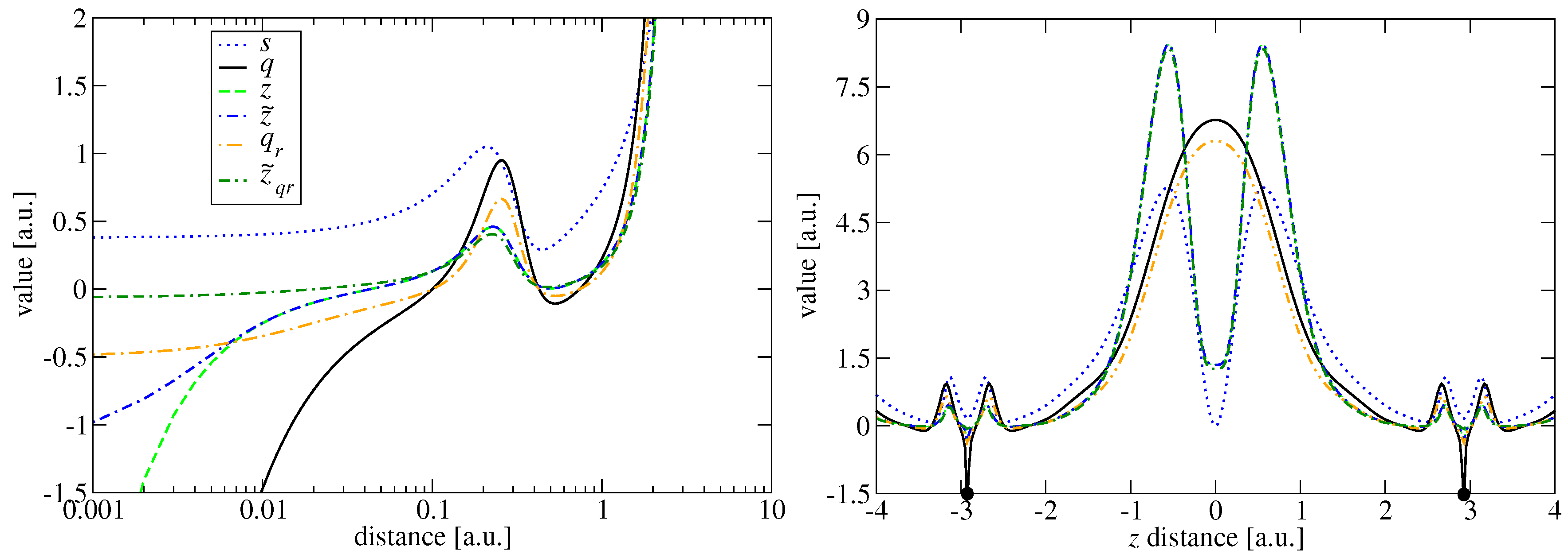
Both ingredients contain information allowing for distinguishing different density regions [51]. This is shown in Figure 1, where we present the spatial behavior of both quantities for two representative systems, namely the Ne atom and the Ne dimer. In the density–tail (where s and ) and slowly varying regions, both quantities are rather proportional to each other. The qualitatively different behavior is more pronounced near the nuclei and in the bond region. In the latter (see the right panel in Figure 1), the reduced gradient goes to zero, whereas .
Similar differences can be noted in the nuclear region. The reduced Laplacian tends here to , while the reduced gradient takes a small, finite value (). The divergence of q may be especially useful to model the deenhancement effect of near the nucleus, which is actually out of reach for standard GGA functionals accurate for the uniform electron gas scaling [52], yielding in this region . We recall that, in large atomic systems, the enhancement factor near nuclei tends to [30]
This feature can be easily recovered by imposing certain restrictions on the enhancement factor form [39].
The description of the approximated KED is not sufficient to model an accurate KE functional. In fact, for applications in OF-DFT and subsystem DFT, the most important quantity to be described is the kinetic potential, which, in the case of the LLMGGA level-of-theory, has the form
The first term in Equation (6) is the TF kinetic potential multiplied by the enhancement factor itself. The second term describes the small correction coming from the variation of w.r.t. the density. The third term is the GGA term, and it can cause some difficulties in GGA functional development i.e., divergences at the nucleus [53] and an unphysical behavior of the corresponding potential in the middle of the bond [54]. Furthermore, it imposes certain conditions on the enhancement factor for which
everywhere in the space. This condition is not satisfied by some KE functionals, e.g., Reference [18]. Finally, the last term in Equation (6) comes from a variation with respect to . This part of the kinetic potential gives rise to major problems, such as unphysical oscillations near the nucleus, or some numerical instability problems related to the high-degree derivatives involved in it (up to ).
As was shown by Cancio et al. [39], the enhancement factor features at the nuclear region can be modeled successfully using a ”hybridization” variable
This inhomogeneity parameter naturally appears in a gradient expansion of the exchange hole, in the regime of a slowly varying density [39,55]. It has been used in the context of XC [56] (with and ) and KE [26] (with and ) functional development to recover the correct behavior of functionals around the nuclei. Here, the a and b parameters in Equation (8) were set to and , according to Reference [39]. When the new ”hybridization” variable z is used, the condition in Equation (7) can be rewritten as .
In the following, we present two new KE functionals, which use a renormalized reduced Laplacian.
2.1. ModAPBEz
In order to construct a KE functional using Equation (8), we start with the modPBE [39] enhancement factor
where , and are parameters. Equation (9) guarantees the finite behavior of the enhancement factor when z diverges. However, it may produce strong unphysical oscillations in the corresponding potential (see the discussion in Section 2.4), due to the term. As it was pointed out in Reference [39], this problem can be partially solved by utilization of a ”renormalized” version of z [26,39]
where C describes the decay rate of the exponential function and is a Heaviside function. Both z and are presented in Figure 1. One can note that, while z exhibits the same features as q in the vicinity of nuclei, the , due to renormalization, approaches the finite negative value .
Following Reference [57], we also introduce the ”renormalized” as
which gives additional control of the kinetic potential curvature and converges to for . The final enhancement factor, named modAPBEz, is:
which has the following limits
The first limit allows for fixing the parameter, in order to recover the modified second-order gradient expansion (MGE2) value of [15]. This can be easily done by substituting Equation (8) into this limit, whereby we find . The last limit can be combined with the Equation (4), to fix the enhancement factor at the nuclei and thus we obtain the relation The remaining parameters C, , and can be chosen through optimization of kinetic potential curvature, in the nuclear region, where we minimize the following integral [39] quantity
for few atomic systems. The optimization of (which is usually responsible for the tail asymptotic behavior of the enhancement factor) together with C can be justified by its strong correlation with value (). It was shown in Reference [39] that the variation of both parameters influences the asymptotic behavior of the enhancement factor given by Equation (9). Thus, setting [39], we perform only the optimization of the remaining two parameters. The optimization of Equation (14) was performed with respect to the He, Ne, and Kr densities obtained from analytical Hartree–Fock orbitals [58]. For each atom, the value of Equation (14) was evaluated (). As a threshold for optimization, we have considered two conditions:
- (i)
- the value of must be of the order a.u.;
- (ii)
- the sum of the absolute differences between the calculated exact KE values () and the approximated ones () satisfies
These conditions have been met for , and so that . The parameter is approximately five times larger than used in the APBE [15] energy functional. Hence, the construction of the modAPBEz meta-GGA KE functional is completed.
2.2. ModAPBEq
Instead of performing a renormalization of the whole z (as in Equation (10)), we can renormalize only the part that actually causes the divergence at the nuclei, namely the reduced Laplacian ingredient. For this purpose, we define a ”renormalized” q as
with the following properties:
- (i)
- when ,
- (ii)
- when ,
- (iii)
- in slowly varying region .
We recall that a quite similar ingredient has been used in the construction of the Laplacian-level EDMGGA exchange functional [56]. In Figure 1, we plotted the for the Ne atom and the Ne dimer. In the tail of density as well as in the middle of the bond, q and behave qualitatively the same.
Then, we define a new ”renormalized” z as
with a and b kept unchanged. One can note, looking at Figure 1, that and behave almost identical in the whole region of space, being superimposed. The major difference only appears in the nuclear region where both variables tend to different finite values, namely and .
Now, substituting in Equation (9), we obtain the new KE functional (denoted here as modAPBEq), which has the following limits
As previously, was set to recover in the slowly varying density limit, and we fixed again . Thus, only is left as a free parameter, which we finally fixed to optimizing w.r.t. subsystem DFT calculations.
Even if modAPBEq does not recover Equation (4), its behavior at the nucleus is still accurate, as shown in the next subsection. Finally, we remark that both modAPBEz and modAPBEq meta-GGA functionals recover the MGE2 in the slowly-varying density limit. This fact insures that they behave correctly under the uniform-electron-gas density scaling [52], and under the Thomas–Fermi density scaling [52,59], then being accurate in the semi-classical limit of large, neural, and non-relativistic atoms [60].
For simplicity, henceforth we will use for modAPBEz and modAPBEq the shortened names mAPBEz and mAPBEq, respectively.
2.3. Comparison of KE Enhancement Factors
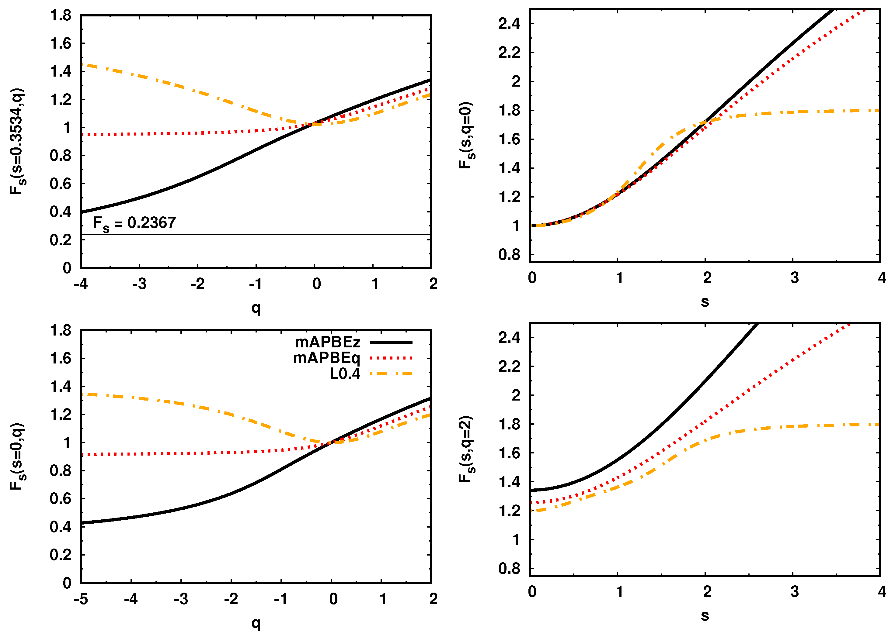
In Figure 2, we present enhancement factors as functions of the reduced Laplacian q (left panels) and reduced gradient s (right panels) for several LLMGGA functionals. The plots are reported for two values of q ( and ) and s (nuclei () and bond ()). The density regime characterized by and negative q is important in the nuclear region.
The L0.4 [25] LLMGGA KE functional shows a large enhancement in this region, which is incorrect from the physical point of view. On the other hand, the mAPBEz goes to the exact deenhancement of Equation (4) and mAPBEq is also less than one.
A similar behavior of enhancement factor can be observed in the bond region where () and q can be either positive or negative (depending on the bond type [61,62]). All GGA KE functionals give here . The L0.4 exhibits a rather strong enhancement for any type of bonding. In case of mAPBEz and mAPBEq functionals, we can note deenhancement for the bond types characterized by the negative value of q.
In the case where (right panels), and , all functionals behave similarly, recovering either MGE2 (as modAPBEz and modAPBEq) or GE4 (as L0.4). For larger values of s (), the functionals start to vary from each other, reaching (for large values of s) the finite value determined by the parameter.
Finally, for a positive value of q (), the shape of L0.4 and mAPBEq enhancement factors for are rather similar, while the mAPBEz functional shows a stronger enhancement.
2.4. Comparison of KE Potentials
As a final element of this section, we discuss the impact of the inclusion of the Laplacian of the density on the quality of the kinetic potentials.
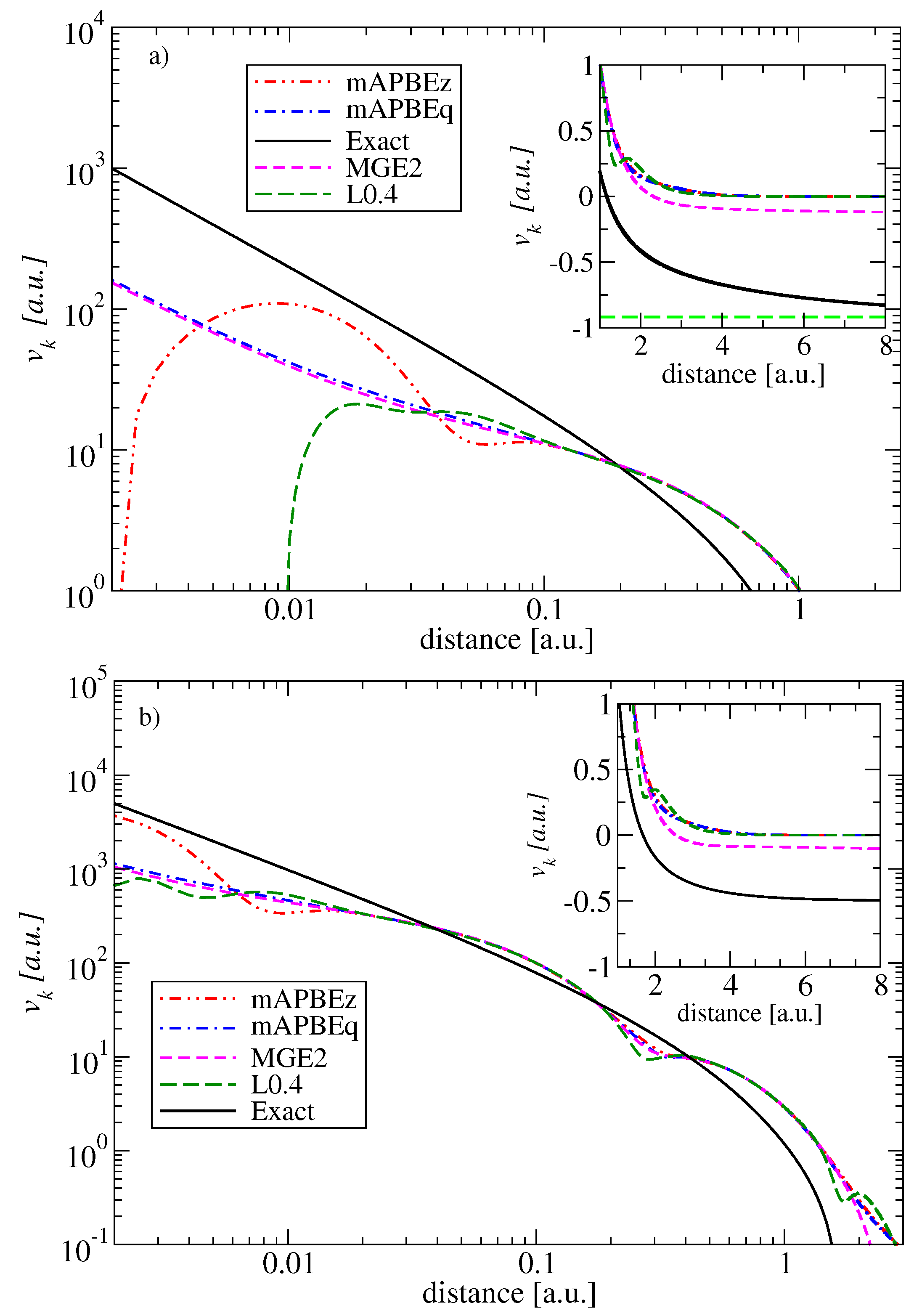
In order to check the overall behavior of the potentials generated by mAPBEz and mAPBEq functionals, we report them in Figure 3 for two representative systems, namely the He and Ne atoms, respectively. Additionally, for comparison, we also plotted the MGE2 and L0.4 [25] potentials. All potentials have been calculated using analytical Hartree–Fock orbitals [58]. The exact potentials are taken from Reference [2].
The figures clearly show a rather poor behavior of all potentials in comparison to ”exact” reference values. Clearly, the errors are larger for the smaller systems, the He atom, for which the exact KE functional is just the von Weizsäcker [63] one, which is not considered in the construction of the present meta-GGA functionals, which have instead increased accuracy with the dimensions of the systems (Recall that MGE2 is exact for an atom with an infinite number of electrons [15]).
The errors are clearly visible both in the core and in long-range asymptotic limit, where the exact kinetic potential approaches the energy of the highest occupied molecular orbitals, in contrast to all meta-GGA functionals considered here which decay to zero. We recall that, in order to improve the overall quality of the kinetic potential, the functional must have a positive Pauli enhancement factor and potential [11,64]. However, by construction of mAPBEz, mAPBEq, and L0.4 meta-GGAs functionals have PBE-like enhancement factors, and, consequently, the von Weizsäcker [63] expression is not recovered asymptotically. However, we recall that our main interest in the present study is the smoothness of the potentials near the core.
In Figure 3, we observe that the mAPBEq potentials are much smoother than the L0.4 and mAPBEz ones, which have large oscillations close to the nucleus (in the case of the He atom, the L0.4 and mAPBEz go to negative values). Instead, the mAPBEq potential is remarkably accurate and as smooth as the MGE2 potential. This fact clearly shows that the renormalized ingredient (see Equation (15)) has important features, being much simpler but also superior to the whole renormalization and smoothness procedures used in the construction of mAPBEz.
3. Computational Details
To enable the comparison of the quality of new functionals, we performed the following benchmark calculations:
- Subsystem DFT calculations: We considered a partition of the total density into two fragments , where and are densities corresponding to subsystems A and B, respectively. The full relaxation of embedded ground-state electron densities was obtained using the freeze-and-thaw cycles [42,43] and considering convergence when the difference of dipole moments of the embedded subsystems is below a.u. In case of KS-DFT calculation, the maximum deviations in density matrix elements of a.u. were considered as convergence criteria. The benchmark set consists of five weakly interacting groups of molecular complexes used in our previous studies [21,45,46].We considered the embedding density error () and the total embedding energy error (). The first is defined aswhere N is the total number of electrons and is the deformation density calculated as the difference between the converged subsystem densities (, ) and the conventional ground state KS density (). In Equation (18), only the valence electron density was considered.
- Atoms: We considered the total KE of few small atoms (aKE test): H, N, C, O, F, Si, P, S, and Cl.
- Molecules: We considered the total KE (mKE test) and the atomization KE (atKE test), of the following small molecules: H, NH, CH, HO, FH, HCN, N, CH, HCO, HOOH, F, SIH, PH, PH, PH, SO, ClF, HCl, SH, Cl, OH, O.
- KE Ionization Potentials (IP) and Electron Affinities (EA): We considered the IP13 and EA13 tests [68], consisting of the following small atoms/molecules C, S, SH, Cl, Cl, OH, O, O, P, PH, PH, S, Si. The KE IP/KE EA has been calculated as the difference between KE of a neutral/changed system minus KE of ionized/neutral species. The errors have been calculated with respect to the values obtained from full KS-DFT calculations.
4. Results
4.1. Subsystem DFT Calculations
The newly defined functionals were employed in subsystem DFT calculations to compute the non-additive KE part of the total energy. The performance of the KE functionals was evaluated using the mean absolute error (MAE) that was calculated for each group of complexes separately. Moreover, to investigate overall performance of KE functionals, we have calculated in the same spirit the relative weighted MAE (rwMAE) [15] defined as
where the sum runs over all group of complexes and is the average MAE calculated for all functionals within each group of systems i. In order to compare our data, we have conducted calculations with several state-of-the-art GGA functionals: revAPBE [15,16], LGAP [21] and one Laplacian-level functional, namely L0.4 [25]. In case of other Laplacian-level KE functionals such as MGE4 or MGGA [23], the use of a monomolecular subsystem DFT approach is required, in order to guarantee good convergence. As was pointed out in Reference [25], the supermolecular approach gives rise to oscillations in the kinetic potential in the tail of the density, therefore causing convergence problems. Hence, those results are not reported in present work. For the same reasons, we do not report in this section the results obtained with the functional proposed in Reference [26], which exhibits the same problems.
In Table 1, we report the errors. First of all, we note that all calculations conducted with mAPBEz and mAPBEq KE functionals provide stable FDE solutions. This is not the case for L0.4 meta-GGA functional where the lack of convergence is observed for five CT complexes. This is the consequence of the aforementioned oscillations [25] in the kinetic potential. Despite this fact, the MAE and rwMAE suggest that the overall performance of both GGAs and meta-GGA KE functionals is rather similar (the rwMAE range between 0.91–1.14). The relatively similar errors suggest that the inclusion of the Laplacian ingredient does not outperform the GGA functionals. This is probably related to the significant cancellation of errors in the non-additive meta-GGA KE functional and potential [25], which are quite similar to those obtained for regular GGAs (see the discussion of Section 2.4). However, at the Laplacian-level of theory, the newly proposed modAPBEq and modAPBEz functionals are better than the L0.4 functional.
Let us turn our attention to the errors that are reported in Table 2. Note that the best overall results are obtained using the mAPBEq functional, which yields a rwMAE of 0.90. It outperforms (in three groups of complexes, namely DI, DHB, and CT) the state-of-the-art revAPBEk and LGAP GGA functionals that both give a total rwMAE of 0.94. The mAPBEq results are closely followed by the ones of the mAPBEz functional, and both overcome the L0.4 functional. Interestingly, in case of DHB complexes, the best MAE (1.14) is provided by the L0.4 KE functional being almost twice as small as those reported by other functionals, but, for all other cases, L0.4 has lower accuracy. In conclusion, mAPBEz and mAPBEq improve over the current state-of-the-art Laplacian-level L0.4 functionals leading to a stable convergence in FDE calculation and providing the results that are in line with current state-of-the-art GGAs.
4.2. Results for Atoms and Molecules
In Table 3, we show the results for small atoms and molecules. All functionals give similar errors for the IP13 and EA13 tests. In this case, the best functional is mAPBEq.
For the other tests (aKE, mKE, and atKE), the best results are found from the APBEk GGA, followed by revAPBEk GGA. All meta-GGAs worsen the total KE of atoms and molecules. Even if mAPBEz has been optimized for He, Ne, and Kr atoms, it is worse than the non-empirical GE4 and L0.4, for both aKE and mKE tests. However, for the atomization KE test (atKE), the mAPBEz and mAPBEq are significantly better than GE4 and L0.4, being as accurate as the revAPBEk GGA. This is the most important result of this subsection, showing that mAPBEz and mAPBEq improve over L0.4 not only for FDE calculations, but also for molecular atomization KE.
5. Conclusions
We have proposed the mAPBEz and mAPBEq Laplacian-level meta-GGA KE functionals, constructed from the mAPBE exchange functional [39], by using the conjointness conjecture hypothesis [40,41]. Both mAPBEz and mAPBEq functionals are similar, and they mainly differ from the renormalization and smoothness procedures used to dump/cancel the non-physical oscillations introduced by the Laplacian of the density, in the kinetic potential close to the nuclear cusp.
However, while mAPBEz uses to the full extent the renormalization and smoothness methods proposed in Reference [39], the mAPBEq is much simpler, being based only on the renormalized reduced Laplacian of Equation (15). Moreover, as shown in Figure 3, the mAPBEq kinetic potential is everywhere remarkably smooth. On the other hand, the mAPBEz kinetic potential still has some unwanted structure at the nuclear cusp. These results fully assess the ingredient that can and should be of interest for further, Laplacian-dependent KE development.
We have tested the mAPBEz and mAPBEq meta-GGA KE functionals in the context of FDE, for a large palette of non-covalently interacting molecular systems, spanning several important classes of forces, such as weak-interaction, dipole–dipole, hydrogen-bond, double-hydrogen-bond, and charge transfer. These functionals improve and extend the applicability over the L0.4 meta-GGA [25], which was the present state-of-the-art Laplacian-level functional for FDE calculations [25]. The overall accuracy of the mAPBEz and mAPBEq is in line with, or even better than, the revAPBEk GGA [15] and LGAP GGA [21]. Finally, we note that the development of LLMGGA is still in its infancy. GGA functionals have been more deeply investigated, but their higher accuracy is based on a strong error compensation on different density regions. Such error compensation can be largely eliminated using the Laplacian ingredient [25], but this task is more difficult to achieve and different paths need to be investigated in the future.
Author Contributions
S.Ś. derived the KE functionals and performed the subsystem DFT calculations. L.A.C. performed numerical calculations for atoms and molecules. S.Ś., E.F., L.A.C. and F.D.S. wrote the manuscript.
Funding
This work was supported by the Polish National Science Center under Grant No. 2016/21/D/ST4/00903.
Conflicts of Interest
The authors declare no conflict of interest.
References
- Wesolowski, T.A.; Wang, Y.A. Recent Progress in Orbital-Free Density Functional Theory; World Scientific: Singapore, 2013. [Google Scholar]
- Wang, Y.A.; Carter, E.A. Orbital-Free Kinetic-Energy Density Functional Theory. In Theoretical Methods in Condensed Phase Chemistry; Springer: Dordrecht, The Netherlands, 2002; pp. 117–184. [Google Scholar] [CrossRef]
- Lignères, V.L.; Carter, E.A. An Introduction to Orbital-Free Density Functional Theory. In Handbook of Materials Modeling: Methods; Springer: Dordrecht, The Netherlands, 2005; pp. 137–148. [Google Scholar] [CrossRef]
- Jacob, C.R.; Neugebauer, J. Subsystem density-functional theory. Wiley Interdiscip. Rev. Comput. Mol. Sci. 2014, 4, 325–362. [Google Scholar] [CrossRef]
- Wesolowski, T.A.; Shedge, S.; Zhou, X. Frozen-Density Embedding Strategy for Multilevel Simulations of Electronic Structure. Chem. Rev. 2015, 115, 5891–5928. [Google Scholar] [CrossRef] [PubMed]
- Banerjee, A.; Harbola, M.K. Hydrodynamic approach to time-dependent density functional theory; Response properties of metal clusters. J. Chem. Phys. 2000, 113, 5614–5623. [Google Scholar] [CrossRef]
- Toscano, G.; Straubel, J.; Kwiatkowski, A.; Rockstuhl, C.; Evers, F.; Xu, H.; Mortensen, N.A.; Wubs, M. Resonance shifts and spill-out effects in self-consistent hydrodynamic nanoplasmonics. Nat. Commun. 2015, 6, 7132. [Google Scholar] [CrossRef]
- Ciracì, C.; Della Sala, F. Quantum hydrodynamic theory for plasmonics: Impact of the electron density tail. Phys. Rev. B 2016, 93, 205405. [Google Scholar] [CrossRef]
- Peverati, R.; Truhlar, D.G. Quest for a universal density functional: The accuracy of density functionals across a broad spectrum of databases in chemistry and physics. Philos. Trans. R. Soc. A 2014, 372, 20120476. [Google Scholar] [CrossRef]
- Scuseria, G.E.; Staroverov, V.N. Progress in the development of exchange-correlation functionals. In Theory and Applications of Computational Chemistry; Elsevier: Amsterdam, The Netherlands, 2005. [Google Scholar]
- Constantin, L.A.; Fabiano, E.; Della Sala, F. Semilocal Pauli–Gaussian Kinetic Functionals for Orbital-Free Density Functional Theory Calculations of Solids. J. Phys. Chem. Lett. 2018, 9, 4385–4390. [Google Scholar] [CrossRef]
- Tran, F.; Wesolowski, T.A. Semilocal Approximations for the Kinetic Energy. In Recent Progress in Orbital-free Density Functional Theory; World Scientific: Singapore, 2013; pp. 429–442. [Google Scholar]
- Lembarki, A.; Chermette, H. Obtaining a gradient-corrected kinetic-energy functional from the Perdew-Wang exchange functional. Phys. Rev. A 1994, 50, 5328–5331. [Google Scholar] [CrossRef]
- Tran, F.; Wesołowski, T.A. Link between the kinetic- and exchange-energy functionals in the generalized gradient approximation. Int. J. Quantum Chem. 2002, 89, 441–446. [Google Scholar] [CrossRef]
- Laricchia, S.; Fabiano, E.; Constantin, L.A.; Della Sala, F. Generalized Gradient Approximations of the Noninteracting Kinetic Energy from the Semiclassical Atom Theory: Rationalization of the Accuracy of the Frozen Density Embedding Theory for Nonbonded Interactions. J. Chem. Theory Comput. 2011, 7, 2439–2451. [Google Scholar] [CrossRef]
- Constantin, L.A.; Fabiano, E.; Laricchia, S.; Della Sala, F. Semiclassical Neutral Atom as a Reference System in Density Functional Theory. Phys. Rev. Lett. 2011, 106, 186406. [Google Scholar] [CrossRef] [PubMed]
- Karasiev, V.V.; Chakraborty, D.; Shukruto, O.A.; Trickey, S. Nonempirical generalized gradient approximation free-energy functional for orbital-free simulations. Phys. Rev. B 2013, 88, 161108. [Google Scholar] [CrossRef]
- Borgoo, A.; Tozer, D.J. Density scaling of noninteracting kinetic energy functionals. J. Chem. Theory Comput. 2013, 9, 2250–2255. [Google Scholar] [CrossRef] [PubMed]
- Xia, J.; Carter, E.A. Single-point kinetic energy density functionals: A pointwise kinetic energy density analysis and numerical convergence investigation. Phys. Rev. B 2015, 91, 045124. [Google Scholar] [CrossRef]
- Della Sala, F.; Fabiano, E.; Constantin, L.A. Kohn-Sham kinetic energy density in the nuclear and asymptotic regions: Deviations from the von Weizsäcker behavior and applications to density functionals. Phys. Rev. B 2015, 91, 035126. [Google Scholar] [CrossRef]
- Constantin, L.A.; Fabiano, E.; Śmiga, S.; Della Sala, F. Jellium-with-gap model applied to semilocal kinetic functionals. Phys. Rev. B 2017, 95, 115153. [Google Scholar] [CrossRef]
- Lehtomäki, J.; Lopez-Acevedo, O. Semilocal kinetic energy functionals with parameters from neutral atoms. Phys. Rev. B 2019, 100, 165111. [Google Scholar] [CrossRef]
- Perdew, J.P.; Constantin, L.A. Laplacian-level density functionals for the kinetic energy density and exchange-correlation energy. Phys. Rev. B 2007, 75, 155109. [Google Scholar] [CrossRef]
- Karasiev, V.V.; Jones, R.S.; Trickey, S.B.; Harris, F.E. Properties of constraint-based single-point approximate kinetic energy functionals. Phys. Rev. B 2009, 80, 245120. [Google Scholar] [CrossRef]
- Laricchia, S.; Constantin, L.A.; Fabiano, E.; Della Sala, F. Laplacian-Level Kinetic Energy Approximations Based on the Fourth-Order Gradient Expansion: Global Assessment and Application to the Subsystem Formulation of Density Functional Theory. J. Chem. Theory Comput. 2014, 10, 164–179. [Google Scholar] [CrossRef]
- Cancio, A.C.; Stewart, D.; Kuna, A. Visualization and analysis of the Kohn-Sham kinetic energy density and its orbital-free description in molecules. J. Chem. Phys. 2016, 144, 084107. [Google Scholar] [CrossRef]
- Constantin, L.A.; Fabiano, E.; Della Sala, F. Performance of Semilocal Kinetic Energy Functionals for Orbital-Free Density Functional Theory. J. Chem. Theory Comput. 2019, 15, 3044–3055. [Google Scholar] [CrossRef] [PubMed]
- Seino, J.; Kageyama, R.; Fujinami, M.; Ikabata, Y.; Nakai, H. Semi-local machine-learned kinetic energy density functional with third-order gradients of electrond ensity. J. Chem. Phys. 2018, 148, 241705. [Google Scholar] [CrossRef] [PubMed]
- Golub, P.; Manzhos, S. Kinetic energy densities based on the fourth order gradient expansion: Performance in different classes of materials and improvement via machine learning. Phys. Chem. Chem. Phys. 2019, 21, 378–395. [Google Scholar] [CrossRef] [PubMed]
- Constantin, L.A.; Fabiano, E.; Della Sala, F. Kinetic and Exchange Energy Densities near the Nucleus. Computation 2016, 4, 19. [Google Scholar] [CrossRef]
- Brack, M.; Jennings, B.K.; Chu, Y.H. On the extended Thomas–Fermi approximation to the kinetic energy density. Phys. Lett. B 1976, 65, 1–4. [Google Scholar] [CrossRef]
- Hodges, C.H. Quantum corrections to the Thomas–Fermi approximation: The Kirzhnits method. Can. J. Phys. 1973, 51, 1428. [Google Scholar] [CrossRef]
- Constantin, L.A.; Fabiano, E.; Della Sala, F. Modified fourth-order kinetic energy gradient expansion with hartree potential-dependent coefficients. J. Chem. Theory Comput. 2017, 13, 4228–4239. [Google Scholar] [CrossRef]
- Zhao, Q.; Levy, M.; Parr, R.G. Applications of coordinate-scaling procedures to the exchange-correlation energy. Phys. Rev. A 1993, 47, 918–922. [Google Scholar] [CrossRef]
- Jemmer, P.; Knowles, P.J. Exchange energy in Kohn-Sham density-functional theory. Phys. Rev. A 1995, 51, 3571–3575. [Google Scholar] [CrossRef]
- Filatov, M.; Thiel, W. Exchange-correlation density functional beyond the gradient approximation. Phys. Rev. A 1998, 57, 189. [Google Scholar] [CrossRef]
- Springborg, M.; Dahl, J.P. On exact and approximate exchange-energy densities. J. Chem. Phys. 1999, 110, 9360–9370. [Google Scholar] [CrossRef] [Green Version]
- Cancio, A.C.; Chou, M. Beyond the local approximation to exchange and correlation: The role of the Laplacian of the density in the energy density of Si. Phys. Rev. B 2006, 74, 081202. [Google Scholar] [CrossRef] [Green Version]
- Cancio, A.C.; Wagner, C.E.; Wood, S.A. Laplacian-based models for the exchange energy. Int. J. Quantum Chem. 2012, 112, 3796–3806. [Google Scholar] [CrossRef]
- Lee, H.; Lee, C.; Parr, R.G. Conjoint gradient correction to the Hartree-Fock kinetic- and exchange-energy density functionals. Phys. Rev. A 1991, 44, 768–771. [Google Scholar] [CrossRef] [PubMed]
- March, N.H. Electron density theory of atoms and molecules. J. Phys. Chem. 1982, 86, 2262–2267. [Google Scholar] [CrossRef]
- Wesolowski, T.A. Chemistry: Reviews of Current Trends; Leszczynski, J., Ed.; World Scientific: Singapore, 2006; Volume 10, pp. 1–82. [Google Scholar]
- Wesolowski, T.A.; Weber, J. Kohn-Sham equations with constrained electron density: An iterative evaluation of the ground-state electron density of interacting molecules. Chem. Phys. Lett. 1996, 248, 71–76. [Google Scholar] [CrossRef] [Green Version]
- Götz, A.W.; Beyhan, S.M.; Visscher, L. Performance of Kinetic Energy Functionals for Interaction Energies in a Subsystem Formulation of Density Functional Theory. J. Chem. Theory Comput. 2009, 5, 3161–3174. [Google Scholar] [CrossRef] [PubMed]
- Śmiga, S.; Fabiano, E.; Constantin, L.A.; Della Sala, F. Laplacian-dependent models of the kinetic energy density: Applications in subsystem density functional theory with meta-generalized gradient approximation functionals. J. Chem. Phys. 2017, 146, 064105. [Google Scholar] [CrossRef] [Green Version]
- Śmiga, S.; Fabiano, E.; Laricchia, S.; Constantin, L.A.; Della Sala, F. Subsystem density functional theory with meta-generalized gradient approximation exchange-correlation functionals. J. Chem. Phys. 2015, 142, 154121. [Google Scholar] [CrossRef] [Green Version]
- Mejia-Rodriguez, D.; Trickey, S. Deorbitalization strategies for meta-generalized-gradient-approximation exchange-correlation functionals. Phys. Rev. A 2017, 96, 052512. [Google Scholar] [CrossRef] [Green Version]
- Thomas, L.H. The calculation of atomic fields. Proc. Camb. Philos. Soc. 1926, 23, 542–548. [Google Scholar] [CrossRef] [Green Version]
- Fermi, E. Un metodo statistico per la determinazione di alcune priorieta dell’atome. Rend. Accad. Naz. Lincei 1927, 6, 602–607. [Google Scholar]
- Fermi, E. Eine statistische Methode zur Bestimmung einiger Eigenschaften des Atoms und ihre Anwendung auf die Theorie des periodischen Systems der Elemente. Zeitschrift für Physik 1928, 48, 73–79. [Google Scholar] [CrossRef]
- Della Sala, F.; Fabiano, E.; Constantin, L.A. Kinetic-energy-density dependent semilocal exchange-correlation functionals. Int. J. Quantum Chem. 2016, 116, 1641–1694. [Google Scholar] [CrossRef]
- Fabiano, E.; Constantin, L.A. Relevance of coordinate and particle-number scaling in density-functional theory. Phys. Rev. A 2013, 87, 012511. [Google Scholar] [CrossRef] [Green Version]
- Staroverov, V.N.; Scuseria, G.E.; Tao, J.; Perdew, J.P. Comparative assessment of a new nonempirical density functional: Molecules and hydrogen-bonded complexes. J. Chem. Phys. 2003, 119, 12129–12137. [Google Scholar] [CrossRef]
- Buksztel, A.; Śmiga, S.; Grabowski, I. The Correlation Effects in Density Functional Theory Along the Dissociation Path. In Electron Correlation in Molecules—ab initio Beyond Gaussian Quantum Chemistry; Hoggan, P.E., Ozdogan, T., Eds.; Academic Press: Cambridge, MA, USA, 2016. [Google Scholar] [CrossRef]
- Becke, A.D. Hartree–Fock exchange energy of an inhomogeneous electron gas. Int. J. Quantum Chem. 1983, 23, 1915–1922. [Google Scholar] [CrossRef]
- Tao, J. Exchange energy density of an atom as a functional of the electron density. J. Chem. Phys. 2001, 115, 3519–3530. [Google Scholar] [CrossRef]
- Cancio, A.C.; Wagner, C.E. Laplacian-based generalized gradient approximations for the exchange energy. ArXiv e-prints 2013, arXiv:1308.3744. [Google Scholar]
- Clementi, E.; Roetti, C. Roothaan-Hartree-Fock atomic wavefunctions: Basis functions and their coefficients for ground and certain excited states of neutral and ionized atoms, Z≤54. Atomic Data Nucl. Data Tables 1974, 14, 177–478. [Google Scholar] [CrossRef]
- Ribeiro, R.F.; Burke, K. Leading corrections to local approximations. II. The case with turning points. Phys. Rev. B 2017, 95, 115115. [Google Scholar] [CrossRef] [Green Version]
- Constantin, L.A.; Snyder, J.C.; Perdew, J.P.; Burke, K. Communication: Ionization potentials in the limit of large atomic number. J. Chem. Phys. 2011, 133, 241103. [Google Scholar] [CrossRef] [PubMed] [Green Version]
- Bader, R.F.W. A Bond Path: A Universal Indicator of Bonded Interactions. J. Phys. Chem. A 1998, 102, 7314–7323. [Google Scholar] [CrossRef]
- Bader, R.F.W.; Essén, H. The characterization of atomic interactions. J. Chem. Phys. 1984, 80, 1943–1960. [Google Scholar] [CrossRef]
- von Weizsäcker, C.F. Zur Theorie der Kernmassen. Z. Phys. A 1935, 96, 431–458. [Google Scholar] [CrossRef]
- Siecinńska, S.; Fabiano, E.; Śmiga, S. About the methods to generate the reference total and Pauli kinetic energy potentials. Unpublished work.
- Laricchia, S.; Fabiano, E.; Della Sala, F. Frozen density embedding with hybrid functionals. J. Chem. Phys. 2010, 133, 164111. [Google Scholar] [CrossRef]
- Weigend, F.; Ahlrichs, R. Balanced basis sets of split valence, triple zeta valence and quadruple zeta valence quality for H to Rn: Design and assessment of accuracy. Phys. Chem. Chem. Phys. 2005, 7, 3297–3305. [Google Scholar] [CrossRef]
- Rappoport, D.; Furche, F. Property-optimized gaussian basis sets for molecular response calculations. J. Chem. Phys. 2010, 133, 134105. [Google Scholar] [CrossRef]
- Zhao, Y.; Truhlar, D.G. The M06 suite of density functionals for main group thermochemistry, thermochemical kinetics, noncovalent interactions, excited states, and transition elements: two new functionals and systematic testing of four M06-class functionals and 12 other functionals. Theor. Chem. Acc. 2008, 120, 215–241. [Google Scholar]
- Weigend, F.; Furche, F.; Ahlrichs, R. Gaussian basis sets of quadruple zeta valence quality for atoms H–Kr. J. Chem. Phys. 2003, 119, 12753–12762. [Google Scholar] [CrossRef]
- Perdew, J.P.; Burke, K.; Ernzerhof, M. Generalized Gradient Approximation Made Simple. Phys. Rev. Lett. 1996, 77, 3865–3868. [Google Scholar] [CrossRef] [PubMed] [Green Version]
- TURBOMOLE V6.2, 2009, a development of University of Karlsruhe and Forschungszentrum Karlsruhe GmbH, 1989-2007, TURBOMOLE GmbH, since 2007. Available online: http://www.turbomole.com (accessed on 10 October 2019).
Figure 1.
The s, q, , z, and inhomogeneity density variable for the Ne atom (left) and Ne dimer (right). The positions of nuclei are indicated by the black dots.
Figure 1.
The s, q, , z, and inhomogeneity density variable for the Ne atom (left) and Ne dimer (right). The positions of nuclei are indicated by the black dots.

Figure 2.
The kinetic energy (KE) enhancement factors for several Laplacian-level meta-GGA (LLMGGA) functionals as a functions of the reduced Laplacian q (left column) and reduced gradient s (right column).
Figure 2.
The kinetic energy (KE) enhancement factors for several Laplacian-level meta-GGA (LLMGGA) functionals as a functions of the reduced Laplacian q (left column) and reduced gradient s (right column).

Figure 3.
The kinetic potentials for the He atom (upper panel) and the Neon atom (lower panel) in a log–log scale. In the insets, the asymptotic regions of the potentials are shown.
Figure 3.
The kinetic potentials for the He atom (upper panel) and the Neon atom (lower panel) in a log–log scale. In the insets, the asymptotic regions of the potentials are shown.


Table 1.
Embedding density errors for subsystem DFT calculations with different KE functionals on several classes of systems. The (nc) denotes non-converged calculations. The mean absolute error (MAE) is indicated for each set of molecules; the global MAE and rwMAE are reported at the bottom of the table. The best results are bolded. ( CT not considered).
| GGAs | metaGGAs | |||||
|---|---|---|---|---|---|---|
| System | revAPBE | LGAP | L0.4 | mAPBEq | mAPBEz | |
| Weak interactions (WI) | ||||||
| He-Ne | 0.05 | 0.09 | 0.22 | 0.06 | 0.08 | |
| He-Ar | 0.06 | 0.07 | 0.22 | 0.10 | 0.12 | |
| Ne-Ne | 0.04 | 0.06 | 0.25 | 0.04 | 0.08 | |
| Ne-Ar | 0.06 | 0.07 | 0.28 | 0.11 | 0.13 | |
| CH-Ne | 0.07 | 0.08 | 0.34 | 0.11 | 0.14 | |
| CH-Ne | 0.13 | 0.15 | 0.28 | 0.19 | 0.22 | |
| CH-CH | 0.60 | 0.71 | 0.37 | 0.81 | 0.86 | |
| MAE | 0.14 | 0.18 | 0.28 | 0.20 | 0.23 | |
| Dipole interactions (DI) | ||||||
| HS-HS | 1.85 | 1.97 | 2.62 | 2.04 | 2.03 | |
| HCl-HCl | 1.87 | 1.89 | 2.22 | 1.94 | 1.97 | |
| HS-HCl | 3.70 | 3.70 | 3.59 | 3.71 | 3.79 | |
| CHCl-Hcl | 2.38 | 2.44 | 2.54 | 2.44 | 2.47 | |
| CHSH-HCN | 1.72 | 1.86 | 2.47 | 1.87 | 1.83 | |
| CHSH-Hcl | 4.08 | 4.11 | 3.81 | 4.10 | 4.18 | |
| MAE | 2.60 | 2.66 | 2.88 | 2.68 | 2.71 | |
| Hydrogen bonds (HB) | ||||||
| NH-NH | 1.79 | 1.97 | 2.68 | 2.05 | 2.02 | |
| HF-HF | 1.53 | 1.51 | 1.76 | 1.54 | 1.56 | |
| HO-HO | 2.01 | 2.08 | 2.53 | 2.14 | 2.14 | |
| NH-HO | 3.11 | 3.22 | 3.58 | 3.26 | 3.26 | |
| HF-HCN | 2.77 | 2.84 | 2.96 | 2.86 | 2.88 | |
| (HCONH) | 2.72 | 2.94 | 3.58 | 2.93 | 2.87 | |
| (HCOOH) | 3.35 | 3.48 | 3.73 | 3.48 | 3.47 | |
| MAE | 2.47 | 2.58 | 2.97 | 2.61 | 2.60 | |
| Dihydrogen bonds (DHB) | ||||||
| AlH-HCl | 5.81 | 5.79 | 5.86 | 5.75 | 5.87 | |
| AlH-HF | 3.82 | 3.80 | 3.29 | 3.74 | 3.83 | |
| LiH-HCl | 14.72 | 14.90 | 16.35 | 14.80 | 14.80 | |
| LiH-HF | 7.58 | 7.68 | 7.40 | 7.58 | 7.59 | |
| MgH-HCl | 4.61 | 4.66 | 4.53 | 4.63 | 4.67 | |
| MgH-HF | 3.21 | 3.23 | 2.97 | 3.18 | 3.23 | |
| BeH-HCl | 3.92 | 3.97 | 3.90 | 3.98 | 4.02 | |
| BeH-HF | 3.42 | 3.40 | 3.13 | 3.36 | 3.44 | |
| MAE | 5.89 | 5.93 | 5.93 | 5.88 | 5.93 | |
| Charge transfer (CT) | ||||||
| NF-HCN | 0.29 | 0.35 | 0.15 | 0.39 | 0.41 | |
| CH-F | 6.35 | 6.32 | 6.43 | 6.33 | 6.34 | |
| NF-HNC | 0.58 | 0.61 | 0.83 | 0.64 | 0.65 | |
| CH-Cl | 5.77 | 5.49 | nc | 5.42 | 5.76 | |
| NH-F | 9.60 | 9.53 | 9.44 | 9.55 | 9.57 | |
| NF-ClF | 1.73 | 1.62 | 1.17 | 1.60 | 1.68 | |
| NF-HF | 0.95 | 0.94 | 0.95 | 0.94 | 0.96 | |
| CH-ClF | 6.02 | 5.66 | nc | 5.56 | 5.97 | |
| HCN-ClF | 3.21 | 3.09 | 3.02 | 3.02 | 3.12 | |
| NH-Cl | 7.60 | 7.23 | nc | 7.17 | 7.60 | |
| HO-ClF | 5.06 | 4.79 | nc | 4.74 | 5.03 | |
| NH-ClF | 11.19 | 13.61 | nc | 15.78 | 12.72 | |
| MAE | 4.86 | 4.94 | - | 5.10 | 4.98 | |
| rwMAE | 0.91 | 0.97 | 1.141 | 0.99 | 1.02 | |
Table 2.
Embedding energy errors (mHa) for subsystem DFT calculations with different GGA and metaGGA KE functionals on several classes of systems. The (nc) denotes non-converged calculations. The mean absolute error (MAE) is indicated for each set of molecules; the global MAE and rwMAE are reported at the bottom of the table. The best results are bolded. ( CT not considered).
| GGAs | metaGGAs | |||||
|---|---|---|---|---|---|---|
| System | revAPBE | LGAP | L0.4 | mAPBEq | mAPBEz | |
| Weak interactions (WI) | ||||||
| He-Ne | 0.08 | 0.15 | 0.23 | 0.13 | 0.11 | |
| He-Ar | 0.05 | 0.13 | 0.23 | 0.10 | 0.08 | |
| Ne-Ne | 0.14 | 0.26 | 0.46 | 0.21 | 0.17 | |
| Ne-Ar | 0.11 | 0.24 | 0.52 | 0.20 | 0.15 | |
| CH-Ne | 0.12 | 0.26 | 0.57 | 0.24 | 0.19 | |
| CH-Ne | −0.03 | 0.20 | 1.45 | 0.30 | 0.17 | |
| CH-CH | −0.38 | −0.24 | 0.96 | −0.15 | −0.27 | |
| MAE | 0.13 | 0.21 | 0.63 | 0.19 | 0.16 | |
| Dipole interactions (DI) | ||||||
| HS-HS | −0.47 | −0.61 | −0.57 | −0.60 | −0.61 | |
| HCl-HCl | 0.07 | −0.10 | 0.06 | −0.07 | −0.09 | |
| HS-HCl | 0.40 | 0.08 | −0.70 | 0.06 | 0.17 | |
| CHCl-HCl | 0.02 | −0.35 | 0.10 | −0.13 | −0.12 | |
| CHSH-HCN | −1.18 | −1.35 | −0.92 | −1.23 | −1.24 | |
| CHSH-HCl | 0.73 | 0.23 | −0.47 | 0.35 | 0.55 | |
| MAE | 0.48 | 0.45 | 0.47 | 0.41 | 0.46 | |
| Hydrogen bonds (HB) | ||||||
| NH-NH | −0.95 | −1.14 | −1.01 | −1.10 | −1.13 | |
| HF-HF | 0.79 | 0.53 | 0.64 | 0.55 | 0.49 | |
| HO-HO | −0.20 | −0.52 | −0.81 | −0.51 | −0.51 | |
| NH-HO | −0.44 | −0.86 | −1.87 | −0.90 | −0.79 | |
| HF-HCN | 0.43 | −0.05 | −1.43 | −0.16 | −0.04 | |
| (HCONH) | −4.21 | −5.37 | −7.43 | −5.16 | −4.89 | |
| (HCOOH) | −1.88 | −3.33 | −7.08 | −3.29 | −2.73 | |
| MAE | 1.27 | 1.69 | 2.90 | 1.67 | 1.51 | |
| Dihydrogen bonds (DHB) | ||||||
| AlH-HCl | 2.54 | 2.01 | −1.18 | 1.71 | 2.06 | |
| AlH-HF | 3.99 | 3.54 | 1.30 | 3.32 | 3.59 | |
| LiH-HCl | 4.63 | 3.83 | −2.01 | 3.14 | 4.05 | |
| LiH-HF | 5.08 | 4.44 | 0.86 | 4.06 | 4.67 | |
| MgH-HCl | 1.79 | 1.29 | −1.36 | 1.04 | 1.34 | |
| MgH-HF | 3.65 | 3.19 | 0.92 | 2.97 | 3.26 | |
| BeH-HCl | 0.70 | 0.42 | −0.73 | 0.30 | 0.37 | |
| BeH-HF | 2.24 | 1.94 | 0.76 | 1.82 | 1.9 | |
| MAE | 3.08 | 2.58 | 1.14 | 2.30 | 2.66 | |
| Charge transfer (CT) | ||||||
| NF-HCN | −0.41 | −0.27 | 1.28 | −0.16 | −0.30 | |
| CH-F | 4.27 | 4.40 | 6.06 | 4.54 | 4.41 | |
| NF-HNC | −0.13 | −0.22 | −0.15 | −0.28 | −0.33 | |
| CH-Cl | 1.52 | 0.71 | nc | 0.94 | 1.64 | |
| NH-F | 6.90 | 6.90 | 8.60 | 7.08 | 6.96 | |
| NF-ClF | 2.14 | 1.85 | 2.21 | 2.08 | 2.12 | |
| NF-HF | 0.91 | 0.69 | 0.35 | 0.63 | 0.62 | |
| CH-ClF | 3.71 | 2.92 | nc | 3.17 | 3.84 | |
| HCN-ClF | 1.62 | 0.97 | −0.10 | 1.21 | 1.53 | |
| NH-Cl | 2.84 | 1.97 | nc | 1.94 | 2.81 | |
| HO-ClF | 2.42 | 1.67 | nc | 1.91 | 2.36 | |
| NH-ClF | 4.44 | 0.86 | nc | 0.63 | 0.87 | |
| MAE | 2.61 | 1.95 | - | 2.05 | 2.32 | |
| rwMAE | 0.94 | 0.94 | 1.37 1 | 0.90 | 0.92 | |
Table 3.
Mean absolute relative errors (MAREs), for the KE of atoms (aKE), KE of molecules (mKE), and mean absolute errors (MAEs) atomization KE (atKE), and the KE ionization potential and electron affinities (IP13-KE and EA13-KE), respectively. We show results for revAPBEk and APBEk GGA functionals, and for GE4, L0.4, mAPBEz, and mAPBEq meta-GGA functionals.
| aKE | mKE | atKE | IP13-KE | EA13-KE | |
|---|---|---|---|---|---|
| revAPBEk | 0.83% | 0.54% | 0.156 | 0.101 | 0.060 |
| APBEk | 0.40% | 0.33% | 0.141 | 0.101 | 0.061 |
| GE4 | 1.60% | 0.98% | 0.264 | 0.104 | 0.064 |
| L0.4 | 1.32% | 0.91% | 0.188 | 0.100 | 0.062 |
| mAPBEz | 1.02% | 0.74% | 0.154 | 0.101 | 0.060 |
| mAPBEq | 1.61% | 1.21% | 0.162 | 0.100 | 0.059 |
© 2019 by the authors. Licensee MDPI, Basel, Switzerland. This article is an open access article distributed under the terms and conditions of the Creative Commons Attribution (CC BY) license (http://creativecommons.org/licenses/by/4.0/).
Share and Cite
MDPI and ACS Style
Śmiga, S.; Constantin, L.A.; Della Sala, F.; Fabiano, E. The Role of the Reduced Laplacian Renormalization in the Kinetic Energy Functional Development. Computation 2019, 7, 65. https://0-doi-org.brum.beds.ac.uk/10.3390/computation7040065
AMA Style
Śmiga S, Constantin LA, Della Sala F, Fabiano E. The Role of the Reduced Laplacian Renormalization in the Kinetic Energy Functional Development. Computation. 2019; 7(4):65. https://0-doi-org.brum.beds.ac.uk/10.3390/computation7040065
Chicago/Turabian StyleŚmiga, Szymon, Lucian A. Constantin, Fabio Della Sala, and Eduardo Fabiano. 2019. "The Role of the Reduced Laplacian Renormalization in the Kinetic Energy Functional Development" Computation 7, no. 4: 65. https://0-doi-org.brum.beds.ac.uk/10.3390/computation7040065
Note that from the first issue of 2016, this journal uses article numbers instead of page numbers. See further details here.