A Holistic Auto-Configurable Ensemble Machine Learning Strategy for Financial Trading

Abstract

Financial markets forecasting represents a challenging task for a series of reasons, such as the irregularity, high fluctuation, noise of the involved data, and the peculiar high unpredictability of the financial domain. Moreover, literature does not offer a proper methodology to systematically identify intrinsic and hyper-parameters, input features, and base algorithms of a forecasting strategy in order to automatically adapt itself to the chosen market. To tackle these issues, this paper introduces a fully automated optimized ensemble approach, where an optimized feature selection process has been combined with an automatic ensemble machine learning strategy, created by a set of classifiers with intrinsic and hyper-parameters learned in each marked under consideration. A series of experiments performed on different real-world futures markets demonstrate the effectiveness of such an approach with regard to both to the Buy and Hold baseline strategy and to several canonical state-of-the-art solutions.

1. Introduction

Nowadays, financial markets represent the backbone of the modern societies, as the world economy is closely related to their behavior [1]. In this context, the investors play a main role, since their decisions drive the financial markets. Differently from the past, nowadays there are several information and communication technologies that have been employed within the financial domain, so investors are now supported by many artificial intelligence instruments that help them to take decisions. Such instruments can exploit a diverse number of techniques [2], from simple statistical approaches to those more sophisticated based on Deep Learning, Social Media Analysis, Natural Language Processing, Sentiment Analysis, and so on [3,4,5,6,7,8].

The literature reports two main methodologies largely used to analyze and predict the behavior of financial markets. The first is based on fundamental analysis, which takes into account the economic elements that may affect the market activities. The second is based on technical analysis [9], which takes into account the historical behavior of the market prices, as it relies on the consideration that the stock prices already include all the fundamental information that could affect it. Moreover, the technical analysis considers the financial asset behavior as a time series, and it is based on the consideration that some behaviors tend to occur again in the future [10,11].

Machine learning solutions have been widely adopted in the context of financial time series forecasting. They usually operate by using a supervised strategy, where classifiers (e.g., Naive Bayes, Decision Trees, Support Vector Machines, etc.) label the data in order to learn their behavior and classify new data into a number of classes (i.e., in the stock market, such classes can be considered as prices going up and down). There are also methods known in statistical analysis that perform regression, which consists of a set of statistical processes for estimating the relationships among variables [12], with the goal of predicting the exact stock price for a day. Although both technical and fundamental data can be used as input data to machine learning approaches, fundamental analysis data do not allow a reliable and high frequency trading for two reasons: (i) these types of information are published at periodic times (e.g., every trimester); and (ii) they are the responsibility of companies, so they can be liable to fraud. Therefore, most of the machine learning approaches do not rely on fundamental information, using diverse other information from technical analysis such as lagged prices, returns, technical indicators, and even news. One more difference between technical and fundamental analysis is that the latter might often use sensitive data (e.g., revenue of companies) and policy procedures should be defined to guarantee privacy, protection, and not disclosure of the data.

In recent years, machine learning approaches have been validated to perform stock market predictions on the basis of historical time series, but, despite the numerous and sophisticated techniques available today, such a task continues to be considered challenging [13]. There are several reasons to explain that: (i) existing methods employ classifiers whose intrinsic parameters are tuned without a general approach but are based on values heavily depending on the used classifier and the target data [4,14]; (ii) the lack of a general technique to set the hyper-parameters (e.g., training and test set sizes, lags, and walks dimension) for the experiments usually makes them not reproducible and thus difficult to assess and to compare with baselines or other approaches [14]; (iii) several works in literature do not specify whether they are performing their test analysis on in-sample or out-of-sample data, and this is a further reason for confusion [4,15,16]; (iv) several works employ classifiers without stating clearly which is the best and under which conditions. This may bring to the common sense that each proposed classifier exploits the peculiarities of the presented market data. Therefore, this does not help understanding whether the method is effective or there are ad hoc classifiers and data choices to report best results only [17,18]; (v) different combinations of feature selection techniques have been explored in financial forecasting, but a framework that can be designed with the goal to get as input any feature and generate the optimal number of output features that is still missing [19]; (vi) for the evaluation step, several metrics have been proposed, but there have not been precise explanations on the adoption of one with respect to the other. This further introduces confusion on the overall analysis and on which metric should be prioritized [20,21,22,23]; and (vii) to define trading strategies, parameters such as those for the data preparation, algorithm definition, training methodology and forecasting evaluation must be the choices to be made by the trading systems architect [1]. To the best of our knowledge, the literature does not offer financial market forecasting approaches based on a systematic strategy, able to model automatically itself with regard to these parameters and chosen market in order to perform well the forecasting task no matter the market considered.

With all of these limitations in mind, we introduce in this paper a general approach for technical analysis of financial forecasting based on an ensemble of predictors automatically created, considering any kind of classifiers and adjustable to any kind of market. In our ensemble, each market will have two sets of parameters tuned: the time series (hyper) parameters and classifier (intrinsic) parameters, no matter the classifiers considered in the ensemble. These parameters are tuned in late past (in-sample) and early past (out-of-sample) datasets, respectively. The input data of such an ensemble are transformed by the Independent Component Analysis, whose parameters are also optimized to make it general enough to return the optimal number of output signals. Therefore, our approach is different from the literature as it is composed of an ensemble of classifiers that can include any classifier and can be maximized for more than one market. To do that, we study the performance of our data-driven ensemble construction by considering different performance metrics in known data in order to tune ensemble parameters over the space of features by using the Independent Component Analysis (ICA) feature selection, parameters (parameters of classifiers, or intra-parameters), and also in the space of time (parameters of the time series). Experiments performed in several futures markets show the effectiveness of the proposed approach with respect to both buy-and-hold strategy and other literature approaches, highlighting the use of such a technique especially by conservative and beginner investors who aim to do safe investment diversification.

The contributions of this paper are therefore the following:

• We formalize a general ensemble construction method, which can be evolved by considering any kind of different classifiers and can be applied to any market.
• We propose an auto-configurable nature, or data-driven nature of such an ensemble. Our approach seeks for hyper (time series) and intrinsic (classifiers) parameters in late and early past data, respectively, generating a final ensemble no matter the market considered.
• We discuss the use of an optimized ICA method as feature selection of the ensemble input, in order to produce the best number of selected features given any number of input signals.
• We perform a performance study by using different metrics based on classification, risk and return, comparing our approach to the well established Buy and Hold methodology and several canonical state-of-the-art solutions.
• In order to reduce the risk that the general strategy optimization phase would lead to results affected by overfitting bias, we systematically rely on the concepts of strictly separated in-sample and out-of-sample datasets for an efficient two-step ensemble parameter tuning, aimed to trade in financial markets.

The remainder of the paper is organized into the following sections. Section 2 introduces basic concepts and related work in stock market forecasting using individual and ensemble approaches. Our self-configurable ensemble method is discussed in Section 3. Section 4 gives details on the experimental environments (datasets), adopted metrics, and implementation details of the proposed method and competitors; Section 5 reports the results on the basis of several metrics in four different markets and, finally, Section 6 provides some concluding remarks and points out some further directions for research where we aim to head as future work.

2. Background and Related Work

The futures market (also known as futures exchange) is an auction market in which investors buy and sell futures contracts for delivery at a specified future date. Some examples of the futures market are the German DAX, the Italian FTSE MIB, the American S&P500, among others. Nowadays, as it happens in almost all markets, all buy and sell operations are made electronically.

In the futures market, the futures contracts represent legal agreements to buy or sell, at a predetermined price and time in the future, a specific commodity or asset. They have been standardized in terms of quality and quantity in order to make easy the trading on the futures exchange. Whoever buys a futures contract assumes an obligation to purchase the underlying asset when the related futures contract expires, whereas whoever sells it assumes an obligation to provide the underlying asset when the related futures contract expires.

Several strategies can be used in order to trade futures contracts. In this paper, we assume an intra-day trading strategy. This methodology to trade stocks, also called day trading, consists of buying and selling stocks and other financial instruments within the same day. In other words, all positions are squared-off (i.e., the trader or portfolio has no market exposure) before the market closes, and there is no change in ownership of shares as a result of the trades. Such a strategy allows the investors to be protected against the possibility of negative overnight events that have an impact on financial markets (i.e., the exit of a country from a commercial agreement, a trade embargo, a declaration of war, and so on). Like other trading strategies, a stop-loss trigger forcing the interruption of the operation when the loss reaches a predetermined value should be adopted to contain risk. Some disadvantages of the intra-day trading strategy are instead the short time available to increase the profit and the commission costs related to the frequent operations (i.e., buy and sell).

Futures market contract prices are published periodically for the general public access. They are usually in the form of comma separated values’ text files, containing the following information: date, open value, highest open value, close value, highest close value, exchange volume. These data are updated in a specific time resolution (5 min, 1 h, 1 day, etc.). This set of observations taken at different times is considered a time series data, and is of crucial importance in many applications related to the financial domain [24,25,26,27,28,29].

Several researchers have explored such time series data with the goal of forecasting future market behavior. The main advantage offered by the approaches based on the technical analysis [9] is related to their capability to simplify the prediction by facing it like a pattern recognition problem. By following this strategy, the input data are given by the historical prices and technical indexes, while the output (forecasting) is generated by using an evaluation model defined on the basis of the past data [15]. Both the statistical and more recent machine-learning-based techniques work by defining their evaluation models considering historical market data as time series. This way, it is possible to analyze the historical data of the stock market, making predictions for the future by using a large number of state-of-the-art techniques and strategies designed to work with time series data [30].

Many machine learning approaches have been deployed in order to analyze this specific kind of time series, which has a non-randomicity and nonlinearity nature [31,32], in order to predict different market prices and returns. Most of these approaches are aimed to predict the single price and/or the prices behavior. The work in [33] used standardized technical indicators to forecast rise or fall of market prices with the AdaBoost algorithm, which is used to optimize the weight of these technical indicators. In [34,35], the authors used an Auto Regressive Integrated Moving Average (ARIMA) in pre-processed time series data in order to predict prices. The authors in [36] proposed a hybrid approach, based on Deep Recurrent Neural Networks and ARIMA in a two-step forecasting technique to predict and smooth the predicted prices. Another hybrid approach is proposed in [37], which uses a sliding-window metaheuristic optimization with the firefly algorithm (MetaFA) and Least Squares Support Vector Regression (LSSVR) to forecast the prices of construction corporate stocks. The MetaFA is chosen to optimize, enhance the efficiency, and reduce the computational burden of LSSVR. The work in [38] used Principal Component Analysis to reduce the dimensionality of the data, Discrete Wavelet Transform to reduce noise, and an optimized Extreme Gradient Boosting to trade in financial markets. The work in [39] validated an extension of Support Vector Regression, called Twin Support Vector Regression, for financial time series forecasting. The work in [40] proposed a novel fuzzy rule transfer mechanism for constructing fuzzy inference neural networks to perform two-class classification, such as what happens in financial forecasting (e.g., buy or sell). Finally, the authors in [41] proposed a novel learning model, called the Quantum-inspired Fuzzy Based Neural Network, for classification. This learning happens using concepts of Fuzzy c-Means clustering. The reader should notice that fuzzy learning is commonly used to reduce uncertainty in the data [42], so such solutions can be useful for financial forecasting. Several other interesting studies have been carried out in the literature, such as a comparison of deep learning technologies to price prediction [43], the use of deep learning and statistical approaches to forecast crisis in the stock market [44], and the use of reward-based classifiers such as Deep Reinforcement Learning [45], among others.

However, it is usually known that single classifiers/hybrid approaches can obtain better performance than that of their single versions when applied in an ensemble model [46,47]. With that in mind, the literature also reports many approaches that exploit a set of different classification algorithms [46,48,49] whose results are combined according to a certain criterion (e.g., full agreement, majority voting, weighted voting, among others). An ensemble process can work in two ways: by adopting a dependent framework (i.e., in this case, the result of each approach depends on the output of the previous one), or by adopting an independent framework (i.e., in this case, the result of each approach is independent) [50]. In this sense, the work in [51] proposed a novel multiscale nonlinear ensemble leaning paradigm, incorporating Empirical Mode Decomposition and Least Square Support Vector Machine with kernel function for price forecasting. The work in [52] fits the same Support Vector Machines classifier multiple times on different sets of training data, increasing its performance to predict new data. The authors of [53] combined results of bivariate empirical mode decomposition, interval Multilayer Perceptrons, and an interval exponential smoothing method to predict crude oil prices. Other interesting approaches using ensembles are the use of multiple feed forward neural networks [54], multiple artificial neural networks with model selection [55], among others.

Notwithstanding, it should be observed that the improvement of ensembles does not represent the norm because certain ensemble configurations can bring a decreasing of the classification performance [56], so a smarter way to select classifiers in the ensemble must be done. Additionally, literature solutions have used ensembles of classifiers with fixed hyper-parameters, such as how to dispose the data to train the ensemble, how to select the parameters of the feature selection approach, among others. In addition, several works employ classifiers without stating with clarity which is the best and under which conditions. This may bring the belief that each classifier exploits peculiarities of the presented market data and, therefore, this does not help with understanding whether the method is effective or the used ensemble has been chosen specifically for the considered market [17,18]. Finally, the use of more diverse classifiers is not extensively studied in the proposed ensembles and neither is a flexible ensemble approach that is adjustable to any kind of market. We show how we tackle these issues with our proposed method in the next section.

3. Proposed Approach

With the previous limitations of literature approaches in mind, we propose in this paper an auto-configurable ensemble, composed of any number of classifiers and adjustable to any market. This ensemble is created automatically after optimizing two sets of parameters: hyper and intrinsic. Once optimized in In-Sample late past (IS) data, hyper-parameters are transferred to the training part of early past data, which we call Out-of-Sample (OOS) data. These hyperparameters will help to find another set of parameters, called intrinsic (classifier) parameters that are optimized in order to update the ensemble of classifiers to more recent data. Then, any new data can be tested. This reduces the problem of creating ad hoc ensembles for specific markets, as our ensemble method outputs a pool of best classifiers for any market as soon the market data are in the IS and training part of OOS sets. Additionally, we allow any number and type of classifiers technologies in the proposed ensemble, minimizing the brute force search for specific classifiers in an ensemble.

Our proposed auto-configurable ensemble is composed of three steps, as follows:

• Feature Selection: data from the target market are pre-processed, with parameters being learned in the IS data.
• Two-Step-Auto Adjustable Parameters Ensemble Creation: with the auto-configurable optimized sets of hyper and intrinsic parameters found in IS data, the approach outputs the set of hyper-parameters only, which will be transferred to a new optimization round. This new optimization step is done in the training part of the OOS data, and will find final intrinsic parameters in recent data to build the final ensemble of classifiers.
• Policy for Trading: we define how to use the created ensemble to trade.

Detailed discussions of these steps are done in the next subsections.

3.1. Feature Selection

In order to reduce noise from the data, the literature reports some approaches able to better generalize the involved information by selecting only the characteristics that best represent the domain taken into account (e.g., the stock market). Although other feature selection techniques could be used by our proposed approach, we considered the Independent Component Analysis (ICA) in our approach, as it was, as far as we know, not fully explored in the financial market context. This feature selection approach is able to extract independent streams of data from a dataset composed of several unknown sources, without the need to know any criteria used to join them [57].

The idea of ICA is to project the d-dimensional input space into a lower dimensional space $d^{\prime }$. It does this by finding a linear representation of non-Gaussian data, so the components are statistically independent. Let us assume a d-dimensional observation vectors $x=\{x_1,x_2,\dots ,x_d\}$ composed of zero mean random variables. Let $s=(s_1,s_2,\dots ,s_d)$ be the d-dimensional transform of x. Then, the problem is to determine a constant weight matrix W so that the linear transformation of the observed variables

$$s=Wx$$

(1)

has certain properties. This means that the input x can be written in terms of the independent components, or

$$x=A^{-1}s,$$

(2)

where A is the inverse (or the pseudo-inverse) of the W transform matrix.

The ICA Based dimensionality reduction algorithm is based on the idea that the features that are least important are the ones whose contribution to the independent components are the least. The least important features are then eliminated and the independent components are recalculated based on the remaining features. The degree of contribution of a feature is approximated as the sum of the absolute values of the transform matrix W entries associated with that feature. The ICA process considers the input data as a nonlinear combination of independent components by assuming that such a configuration is true in many real-world scenarios, which are characterized by a mixture of many nonlinear latent signals [58,59]. A more rigorous formalization of ICA is provided in [60], where it has adopted a statistical latent variables model. It assumes that we observe n linear mixtures of n independent components.

In our optimized ICA approach, we select the best possible number of parameters to be used by this technique, no matter the market considered. This is done by adjusting hyper-parameters, a step further discussed in the next subsection.

3.2. Two-Step Auto Adjustable Parameters’ Ensemble Creation

This section discusses the proposed method of generating automatically an ensemble of several classifiers to trade in any kind of market. We start by giving an overview of the approach; then, we show how we perform optimization of parameters and, finally, we describe the parameters to be learned in order to output the final ensemble.

3.2.1. Overview

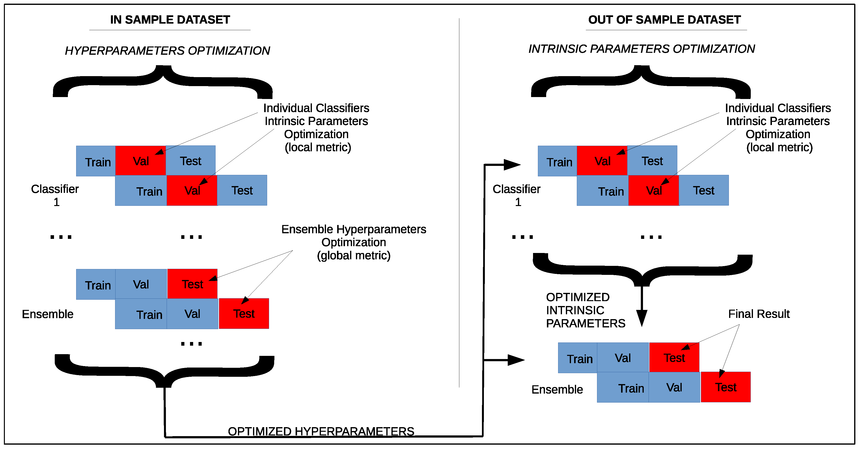
Our method is a self-configurable ensemble of classifiers whose pipeline can be seen in Figure 1. In our approach, hyperparameters (time-series-based) are optimized through performances metrics calculated for the ensemble in the IS data, and are transferred to the training set of OOS (more recent past) data. Finally, intrinsic (classifiers) parameters are found for the classifiers of the final ensemble, considering more recent past data and the ensemble is updated to test any kind of new data.

The performance metrics we consider in our study lie within the machine learning and the economic domains. The rationale behind that is that, in addition to a mere evaluation of the percentage of correct predictions (i.e., accuracy), it is also necessary to estimate the impact of them at the economic level. For instance, the measurement of a good accuracy in the predictions related to a period of five years is not significant if, for some intervals of this period (e.g., two consecutive years), we suffered huge economic losses that, certainly, in a real-world scenario, would have stopped any further investment. For this reason, together with the Accuracy metric, we adopted as evaluation metrics the Maximum Drawdown, the Coverage, and the Return Over Maximum Drawdown, whose formalization will be provided later in Section 4.2.

To illustrate the benefits of our proposed auto-configurable ensemble method, we build it considering three basic state-of-the-art classifiers [3,61,62]: Gradient Boosting (GB), Support Vector Machines (SVM), and Random Forests (RF), although any other kinds of classifiers may either replace those or be plugged in. Our method has two sets of parameters to be learned, through a methodology described in detail in the next subsection.

3.2.2. Walk-Forward Optimization

One of the most used optimization approaches within a financial forecasting process for the detection of the best parameters to adopt in the trading strategy is called Walk Forward Optimization (WFO) [63]. We adopt such a strategy to find the best ensemble hyperparameters in the IS data and intrinsic parameters in part of OOS data. It works by isolating the IS time series into several segments, or walks, where each segment is divided in two parts: Training and Testing sets. The parameters optimization for the used trading strategy is then performed by (i) using several combinations of parameters to train the model in the training part of a segment; and (ii) declare the best (optimized) parameters the ones that yield best performance in the testing set of the same segment. The process is then repeated on the other segments. The performance obtained in the testing set of each segment is not biased as we are not using unknown data, but just IS data. The Walk Forward Optimization can be performed by following two methodologies, described as follows:

• Non-anchored Walk Forward Optimization: this approach creates walks of the same size. For example, let us assume we have a dataset composed of 200 days that we want to divide into six walks of 100 days. One way is to consider the first 80 days of each walk as the training set and the remaining 20 days as the testing set, as shown on the left side of

  Table 1. Non-anchored and Anchored Walk Forward Optimization.

  Data	Non-Anchored WFO			Anchored WFO
  Segment/Walk	Training	Testing	Days	Training	Testing	Days
  1	$1\to 80$	$81\to 100$	100	$1\to 80$	$81\to 100$	100
  2	$21\to 100$	$101\to 120$	100	$1\to 100$	$101\to 120$	120
  3	$41\to 120$	$121\to 140$	100	$1\to 120$	$121\to 140$	140
  4	$61\to 140$	$141\to 160$	100	$1\to 140$	$141\to 160$	160
  5	$81\to 160$	$161\to 180$	100	$1\to 160$	$161\to 180$	180
  6	$101\to 180$	$181\to 200$	100	$1\to 180$	$181\to 200$	200

  .
• Anchored Walk Forward Optimization: in this scenario, the starting point of all segments is the same. Additionally, the training set of each segment is longer than the training set of the previous one; therefore, the length of each walk is longer than the length of the previous one, as shown on the right side of Table 1.

In our approach, we consider the non-anchored modality of the Walk Forward process, a widely used approach in the literature for financial markets [64]. Additionally, the non-anchored WFO used in our approach further subdivides the training data in Table 1 into training and validation data, where the validation data are 30% of the training data. Then, the performance in the validation data will help find a set of intrinsic parameters of the classifiers of the ensemble, whereas the performance in the testing data will find the hyper-parameters of the ensemble. We discuss such auto-configurable parameters in the next section.

3.2.3. Transferable Self Configurable Parameters

With the information of the classifiers used and the optimization methodology in mind, we finally describe the parameters to be found in order to generate the final ensemble. The first set of parameters to be learned through non-anchored WFO comes from the classifiers and are reported in

Table 2. Intra-parameters grid.

Algorithm	Parameter	Values	Description
$GradientBoosting$	$n\_estimators$	$10,25,50,100$	Boosting stages to perform
	$learning\_rate$	$0.0001,0.001,0.01,0.1$	Contribution of each tree
	$max\_depth$	$2,4,6,8,10$	Maximum depth of each estimator
$SupportVectorMachines$	$max\_iter$	$20,50,100$	Hard Limit on iterations within solver
	$tol$	$0.0001,0.001,0.01,0.1$	Tolerance for stopping criterion
	C	$1,10,20,50$	Penalty of the error term
	$gamma$	$0.0001,0.001,0.01,0.1$	Coefficient for the used kernel
$RandomForests$	$n\_estimators$	$20,50,100$	Trees in the forest
	$max\_depth$	$1,5,10,50$	Maximum depth of the tree
	$min\_samples\_split$	$0.2,0.4,0.8,1.0$	Minimum samples to split an internal node

, along with a list of values that must be grid searched within the process. Other values and even other parameters can be added too, making the classifiers even more robust to the uncertainties in the training data. Such values are optimized according to the performances in the validation data, a fraction of the training data discussed before in Section 3.2.2.

The second set of parameters to be tuned is represented by the hyper-parameters, which are not from the classifiers anymore, but are related to the non-anchored WFO and ICA feature selection.

Table 3. Hyper-parameters grid.

Parameter	Values	Description
$window\_size$	$100,150,200,250,300$	Days used for the training and test sets definition
$train\_size$	$60,65,70,75,80$	Percentage of window_size used for the training set
$lags$	$1,3,5,7,9$	Previous days to use in order to predict the next one
$ica\_comp$	$1,3,5,7,9$	Independent Component Analysis output components

shows the hyper-parameters that need to be optimized according to the chosen metric. They are (i) the dimension of the window for each walk; (ii) the training set size; (iii) lag size; and (iv) number of output signals of the considered ICA feature selection approach. These hyper-parameters are optimized through the chosen performance metrics after ensemble classification of testing data, where $test\_size=window\_size-train\_size-validation\_size$. These hyperparameters’ self-configuration step of our approach is carried out only within the IS part of our dataset, according to a considered metric. Once the hyperparameters and intrinsic parameters are found in the IS data, the algorithm transfers the hyperparameters only to the OOS dataset. Then, only the intrinsic parameters of the ensemble are optimized and, thus, the ensemble is ready to test new data.

Algorithm 1 describes the proposed approach of multi-classifiers’ auto-configurable ensemble. The algorithm has three main variables: (i) $MAX\_FINAL\_METRIC$ (initialized in step 7 of the algorithm), which will be used in step 28 to check which hyperparameter $h\in H$ has the best ensemble performance metric; (ii) $ENS\_METRICS$ (initialized in step 8 of the algorithm), which will sum up the metric of applying the ensemble in test part of IS data in all walks; and (iii) $MAX\_WALK\_METRIC$ (initialized in step 14 of the algorithm), which will be used to optimize classifiers intrinsic parameters in the validation data of each walk. The algorithm starts by, given a combination of hyperparameters $h\in H$, building the walks W (step 10) and, for each walk $w\in W$, it builds and transforms features (steps 12 and 13), doing a grid search in all the classifiers’ intrinsic parameters combinations $i\in I$ in order to find the best classifier for each walk (steps 16–22). After the best of each classifier is found for a walk, we apply the ensemble of them accumulating the performance metric in the testing data for all the walks (step 26). After this is done for each hyperparameter combination, we verify, in steps 28–30, if the total metric of the ensemble in all the walks is the highest possible. When all the hyperparameter combinations h have their ensemble tested and with their accumulated metrics on the testing data calculated, in step 33, the algorithm is sure that it found the best possible hyperparameter $h^{\prime }\leftarrow H$, which is returned by the algorithm.

After the hyperparameters are found in the IS data, we start the search for the intrinsic parameters of the ensemble in recent past data, and then our ensemble is ready and can already trade. Such procedure is reported in Algorithm 2. In this algorithm, just two metrics are necessary: (i) the variable $MAX\_WALK\_METRIC$ (step 12 of the algorithm) to tune the intrinsic parameters of the classifiers in the new OOS data; and (ii) $METRIC$ (step 8 of the algorithm) to calculate the final metrics of the ensemble trading on unseen OOS data. The process is similar to Algorithm 1, with the difference being the fact that hyperparameters are not searched anymore and the testing data are used to report trading real-time results. The algorithm returns the mean metric, considering the whole testing period.

Algorithm 1 Proposed hyperparameter search approach.

Require: 1: $IS$ = time series from in sample data 2: I = list of intra-parameters as shown in Table 2 3: H = list of hyperparameters as shown in Table 3 4: C = list of classifiers from the ensemble Ensure: 5: $h^{\prime }$ = Optimized hyperparameters 6: procedureReturn_Hyperparameters($IS$, I, H, C) 7:     $MAX\_FINAL\_METRIC\leftarrow 0$ 8:     $ENS\_METRIC\leftarrow 0$ 9:     for h in H do                                  ▹for each hyperparameter combination 10:         $W\left[h\right]\leftarrow buildWalks(IS,h(window\_size\left)\right)$                 ▹ Starts non-anchored WF0 11:         for w in $W\left[h\right]$ do                                         ▹ for each walk 12:            $F\leftarrow buildFeatures(w,h(lags\left)\right)$                                 ▹ get features 13:            $F^{\prime }\leftarrow icaTransform(h(ica\_comp),F)$                   ▹ transform features 14:            $MAX\_WALK\_METRIC\leftarrow 0$ 15:            for c in C do                                       ▹ for each classifier 16:                for i in I do                    ▹ for each intrinsic parameter, train and validate 17:                    $M\left[i\right]\leftarrow trainClassifier(F^{\prime },h(train\_size),c\left[i\right])$ 18:                    $METRIC\leftarrow testClassifier(M\left[i\right],F^{\prime }[h(train\_size)*0.3])$ 19:                    if $METRIC>MAX\_WALK\_METRIC$ then 20:                        $E[c,w]\leftarrow M\left[i\right]$ 21:                        $MAX\_WALK\_METRIC\leftarrow METRIC$ 22:                    end if 23:                end for 24:            end for 25:            $test\_data\leftarrow F^{\prime }[h(window\_size)-h(train\_size)-h(train\_size)*0.3]$ 26:            $ENS\_METRIC\leftarrow ENS\_METRIC+testClassifier\left(E\right[C,w],test\_data)$ 27:         end for 28:         if $ENS\_METRIC>MAX\_FINAL\_METRIC$ then 29:            $h^{\prime }\leftarrow h$ 30:            $MAX\_FINAL\_METRIC\leftarrow ENS\_METRIC$ 31:         end if 32:     end for 33:     return $h^{\prime }$ 34: end procedure

Algorithm 2 Proposed intrinsic parameter search approach and ensemble trading

Require: 1: $OOS$ = time series from in sample data 2: I = list of intra-parameters as shown in Table 2 3: $h^{\prime }$ = best hyperparameter found in Algorithm 1 4: C = list of classifiers from the ensemble Ensure: 5: $MEAN\_METRIC$ = Mean performance of trading 6: procedureEnsemble_Trading($OOS$, I, $h^{\prime }$, C) 7:     $W\leftarrow buildWalks(OOS,h^{\prime }(window\_size))$                     ▹ Starts non-anchored WFO 8:     $METRIC\leftarrow 0$                                   ▹ Metric used to report testing results 9:     for w in Wdo                                                ▹for each walk 10:         $F\leftarrow buildFeatures(w,h^{\prime }\left(lags\right))$                                   ▹ get features 11:         $F^{\prime }\leftarrow icaTransform(h^{\prime }(ica\_comp),F)$                       ▹ transform features 12:         $MAX\_WALK\_METRIC\leftarrow 0$ 13:         for c in Cdo                                      ▹ for each classifier 14:            for i in I do                           ▹ for each intrinsic parameter, train and validate 15:                $M\left[i\right]\leftarrow trainClassifier(F^{\prime },h^{\prime }(train\_size),c\left[i\right])$ 16:                $METRIC\leftarrow testClassifier(M\left[i\right],F^{\prime }[h^{\prime }(train\_size)*0.3])$ 17:                if $METRIC>MAX\_WALK\_METRIC$ then 18:                    $E[c,w]\leftarrow M\left[i\right]$ 19:                    $MAX\_WALK\_METRIC\leftarrow METRIC$ 20:                end if 21:            end for 22:         end for 23:         $test\_data\leftarrow F^{\prime }[h^{\prime }(window\_size)-h^{\prime }(train\_size)-h^{\prime }(train\_size)*0.3]$ 24:         $METRIC\leftarrow METRIC+testClassifier\left(E\right[C,w],test\_data)$ 25:     end for 26:     $MEAN\_METRIC\leftarrow METRIC/\left|W\right|$ 27:     return $MEAN\_METRIC$ 28: end procedure

Doing the search of parameters this way, the hyper-parameters of the final ensemble will be optimized in the IS data through non-anchored WFO. Then, these hyperparameters are transferred to the non-anchored WFO of the OOS data, and intrinsic parameters are now optimized in the validation data only. Thus, an auto adjustable ensemble approach is built in such a way that will return an ensemble of the best possible classifiers for any market, as long as their IS and training and validation OOS data are fed to the algorithm, being this way a data-driven optimization approach.

3.3. Policy for Trading

Many literature studies [65,66] demonstrate the effectiveness of ensemble approaches that implement different algorithms and feature subsets. Ensemble approaches [67] usually get the best results in many prestigious machine learning competitions (e.g., Kaggle, Netflix Competition, KDD, and so on).

Therefore, in this paper, we are adopting an ensemble learning approach, which means that the final result (i.e., the prediction) is obtained by combining the outputs made by single algorithms in the ensemble. As stated before in Section 2, such an ensemble process can work in a dependent or independent fashion. The approach we choose is the independent framework, so each classifier decision may represent a vote that is independent from the others. We apply such an approach using three selected algorithms (i.e., Gradient Boosting, Support Vector Machines, and Random Forests) with their ensemble hyperparameters initially found in the IS data, and whose individual classifiers intrinsic parameters are found in the OOS data. We adopt in our ensemble approach the aggregation criterion called complete agreement, meaning that we make our prediction to buy or sell only if there is a total agreement among all the algorithm predictions, otherwise we do not make a prediction for the related futures market (hold). This is an approach that usually leads towards better predictive performance, compared to that of each single algorithm. Such an approach for the future day prediction is better illustrated in Algorithm 3.

Algorithm 3 Future day prediction

Require:A = Set of algorithms, D = Past classified trading days, $\widehat{d}$ = Day to predict Ensure:$result$ = Day $\widehat{d}$ prediction 1: procedurePrediction(A, D, $\widehat{d}$) 2:     $models=trainingModels(A,D)$ 3:     $predictions=getPredictions(models,\widehat{d})$ 4:     if $agreement\left(predictions\right)$ == $TRUE$ ∧ $predictions$ == $-1$ then 5:         $result$←$sell$ 6:     else if $agreement\left(predictions\right)$ == $TRUE$ ∧ $predictions$ == 1 then 7:         $result$←$buy$ 8:     else 9:         $result$←$hold$ 10:     end if 11:     return $result$ 12: end procedure

4. Experimental Setup

In this section, we discuss the setup chosen to guide the experiments performed to validate our ensemble approach against some baselines from the literature. We start discussing the datasets, the performance metrics, and implementation aspects of our proposed method and of the competitors.

4.1. Datasets

To verify our approach performance against some baselines, we selected four datasets based on stock futures markets (SP500, DAX and FIB) and one future of commodity (CL). As far as the stock futures markets are concerned, we included the FIB market, which is characterized by an atypical behavior with respect to the other stock futures markets in the years taken into account during the experiments. We based our choice on the observation that stock markets behavior is usually different from that of the bond markets, as there usually exists an inverse correlation between them. Indeed, the stock futures are frequently characterized by a strong upward bias (e.g., SP500 and DAX), with some exceptions related to some particular economic scenarios, as it happened for the Italian FIB in recent years. Details of such datasets are reported in

Table 4. Futures Market Datasets.

Futures	Name	From	To	Trading
Dataset		Day	Day	Days
$SP500$	Standard & Poors 500	$02/01/2008$	$31/12/2018$	2827
$DAX$	German Market	$02/01/2008$	$28/12/2018$	2792
$FIB$	Italian Market FIB Future	$02/01/2008$	$27/12/2018$	2790
$CL$	Light Sweet Crude Oil Future	$02/01/2008$	$28/12/2018$	2774

.

These datasets can be easily found at different time resolutions (e.g., 5-min, 10-min, 1-h, etc.). In this work, we further transform the futures market datasets by adopting a 1-day resolution. It means that, starting from the original resolution that characterizes the dataset (e.g., 5-min, 10-min, 1-h, among others), the data have been opportunely joined in order to obtain for each day included in the dataset the following new information I = {date, open value, highest value, lowest value, close value, exchange volume}, where each record of the new dataset corresponds to one day. As the SP500 market has a point value of 50 USD, the DAX market has a point value of 25 EURO, the FIB market has a point value of 5 EURO and the CL market has a point value of 1000 USD, in order to simplify, we do not convert the points to their corresponding currency values, keeping such information in points.

In these datasets, we denote a set of data composed of a series of consecutive trading days as $X=\{x_1,x_2,\dots ,x_N\}$, and a set of features $F=\{date,open,high,low,close,volume,next\}$ that compose each $x\in X$ and $next=1$ if the $close-open$ of the next day is greater than or equal to zero, and $next=-1$, otherwise. We also label the buy operation to 1, and sell operation to $-1$, as they represent the operations allowed on the futures markets taken into consideration in this paper.

It should be observed that, according to the aforementioned definition of $next\in F$, a trading day can only belong to one class $c\in C$, where $C=\{1,-1\}$. We also denote as $I=\{i_1,i_2,\dots ,i_X\}$ the components of each trading day $x\in X$, obtained by transforming the original data through a feature selection process, which in our case is ICA. Finally, we denote a set of of operations $O=\{buy,sell,hold\}$ allowed on a futures market, where $hold$ means that no operation of buy or sell has been performed. The reader notices that a buy operation corresponds to a long trade ($C=1$), where a trader buys an asset hoping the price will go up at the end of the day. On the other hand, a sell operation corresponds to a short trade ($C=-1$). In such a case, a trader sells an asset before buying it hoping that its price will go down.

Given the previous definitions, for each trading day x (i.e., each dataset row), we add a further data field next, which corresponds to the target class related to the next trading day $x+1$, and is defined according to the notation reported in Equation (3):

$$\begin{array}{c}nex{t}_x=\left\{\begin{array}{cc}\mathit{1},\hfill & \mathrm{if}(clos{e}_{x+1}-ope{n}_{x+1})\ge 0,\hfill \\ -\mathit{1},\hfill & \mathrm{otherwise}.\hfill \end{array}\right.\hfill \end{array}$$

(3)

We let the reader observe that the time series resolution may be set even to a finer scale, e.g., hours or minutes. In such a case, a record in a given time interval would consist of a group features {time, open value, highest value, lowest value, close value} for each considered interval, ended with the next class, as defined above.

To train our prediction models with more than a day of the features market (lags hyper-parameter in Table 3), we can arbitrarily aggregate more days, obtaining a series of vectors V composed of ICA components of N days, with the next value as target class. As an example, assuming we have to aggregate three days $x_1,x_2,x_3$, each of them characterized by two ICA components $i_1,i_2$, we would obtain the vector shown in Equation (4):

$$V=[x_1\left(i_1\right),x_1\left(i_2\right),x_2\left(i_1\right),x_2\left(i_2\right),x_3\left(i_1\right),x_3\left(i_2\right),nex{t}_{x_4}].$$

(4)

In our experiments, we report the experiments considering the period from 2016 to 2018 as OOS data, where we have updated and tested our approach after the auto-configuration and tuning of the hyperparameters in the IS data, which uses the remaining years.

4.2. Evaluation Metrics

In this subsection, besides the canonical performance evaluation metrics such as Accuracy, we added in our study other financial performance metrics, such as Maximum Drawdown, Coverage, Return Over Maximum Drawdown, and Equity Curve. In the following, we detail each of them.

4.2.1. Accuracy

This metric gives us information about the number of instances correctly classified, compared to the total number of them. It provides an overview of the classification performance. Formally, given a set of X closing trading days to be predicted, it is calculated as shown in Equation (5), where $\left|X\right|$ stands for the number of trading days and $X^{(+)}$ stands for the number of those correctly classified:

$$Accuracy\left(X\right)={\displaystyle \frac{X^{(+)}}{\left|X\right|}}.$$

(5)

As our approach only acts in the market when there is a total agreement of votes between the classifiers considered, we calculate the accuracy only when our proposed ensemble takes decisions (i.e., no hold operations are done). This happens because our trader does not enter the market all the time, so the accuracy of our trader is considered a different metric than the same used for baselines, which enter the market all the time. Therefore, we use the accuracy metric in the experiments not for benchmarking all approaches, but rather for two tasks: (i) compare the individual original and boosted classifiers in order to highlight the benefits of the data-driven nature of our approach; and (ii) assess the accuracy of our proposed approach according to its total trading actions in the market.

4.2.2. Maximum Drawdown (MDD)

Such a metric represents the largest drop from a peak to a trough before a new peak is reached. It indicates the downside risk in a the time period taken into account [68]. A low maximum drawdown is preferred as this indicates that losses from investment were small. If an investment never lost a penny, the maximum drawdown would be zero. Formally, denoting as P the peak value before the largest drop, and as L the lowest value before a new high is established, its formal notation can be simplified as shown in Equation (6):

$$MDD={\displaystyle \frac{(P-L)}{P}}.$$

(6)

As stated before, low MDDs mean that losses in a trading strategy are low. Therefore, we use the Maximum Drawdown in our experiments as a measure to quantify how risky are the algorithms evaluated.

4.2.3. Coverage (COV)

The coverage metric reports the percentage of times we carried out an operation [69] (i.e., buy or sell) on the futures market (i.e., $\left|buy\right|+\left|sell\right|$) compared to the number of days taken into consideration (i.e., $\left|X\right|$), as shown in Equation (7). It gives us important information, since in addition to predicting a buy or sell operation, an algorithm can also predict to not buy and not sell anything (hold):

$$COV={\displaystyle \frac{\left(\right|buy|+|sell\left|\right)}{\left|X\right|}}.$$

(7)

In our experiments, we use the $COV$ metric to quantify how many times our proposed trading system decides to act in the market (i.e, perform Long or Short operations).

4.2.4. Return over Maximum Drawdown (RoMaD)

The RoMaD is a metric largely used within the financial field in order to evaluate the gain or loss in a certain period of time, such as the Sharpe Ratio or the Sortino Ratio [70,71]. More formally, it represents the average return for a portfolio expressed as a proportion of the Maximum Drawdown level, as shown in Equation (8), where Portfolio Return denotes the difference between the final capital and the initial one:

$$RoMaD={\displaystyle \frac{PortfolioReturn}{MDD}}.$$

(8)

In practice, investors want to see maximum drawdowns that are half or less the annual portfolio return. This means that, if the maximum drawdown is 10% over a given period, investors want a return of 20% (RoMaD = 2).

4.2.5. Equity Curve

The Equity Curve (EC) reports the change in the value of a trading account in the time period graphically [72]. A significant positive slope usually indicates the effectiveness of the adopted trading strategy, while negative slopes indicate that such a strategy generates negative returns. For instance, given an Initial Investment II to trade a number of futures that have a certain entry price and exit price, and also considering the related trade commission, we can calculate the points $EC=\{e{c}_1,e{c}_2,\cdots ,e{c}_N\}$ that we need to plot in the Equity Curve as shown in Equation (9):

$$\begin{array}{c}e{c}_1=II-((entryprice\times numberoffutures)-commission)\hfill \\ e{c}_2=II-((exitprice\times numberoffutures)-commission)\hfill \\ ⋮\hfill \\ e{c}_{N-1}=II-((entryprice\times numberoffutures)-commission)\hfill \\ e{c}_N=II-((exitprice\times numberoffutures)-commission).\hfill \end{array}$$

(9)

We use the EC in our experiments to compare the evolution of gains and losses of all the evaluated algorithms over time.

4.3. Technical Details

The approach proposed in this paper has been developed in Python, as well as the implementation of the state-of-the-art classification techniques used to define our ensemble approach, which are based on scikit-learn (http://scikit-learn.org). In order to make our experimental results reproducible, we have set to zero the seed of the pseudo-random number generator used by the scikit-learn evaluation algorithms. The machine where all the experiments have been performed is an Intel i7-3770S, octa-core(3.10 GHz × 8) with a Linux 64-bit Operating System (Debian Stretch) with 8 GB of RAM.

As for the competitors, we firstly considered the common Buy and Hold baseline strategy. It represents a passive investment strategy in which the investors buy futures and hold them for a long period, regardless of the market’s fluctuation. Such a strategy is largely used in literature as a baseline to evaluate the profitability of an investment strategy. In addition, we performed the future market predictions by using single predictors (i.e., GB, SVM, and RF), configuring their default hyper-parameters according to some common values in the literature: $40\%$ of the IS dataset as walk size, of which $75\%$ is used as training set and the remaining $25\%$ as validation set with 5 day-lags [15,16,73,74,75]. Finally, we also used a recent approach to perform trading [39], which we call TSVR in the remaining of this paper. For this approach, we used both the linear (LIN) and nonlinear (NONLIN) kernel. As described in in [39], we have used 10-fold cross validation in the training data to find the kernel parameters that yielded the best mean squared error in all markets. As this approach is proposing to predict the closing price (regression problem), we mapped the problem consistently with ours and changed the output so that for each day we have either a long or short operation. As with our approach, final results are reported in terms of classification performance in the testing part of the OOS dataset.

Regarding time consumption related to our approach, we can observe from the pipeline showed in Figure 1 that it is strictly related to the canonical time spent by each algorithm that composes the ensemble, multiplied by the intrinsic parameters involved in the auto-tuning process plus the time spent by other processes (i.e., walk-forward and ICA Feature Selection), since the detection process of the optimal hyper-parameters has been previously (one time) performed in the in-sample part of the datasets; therefore, it does not need to be repeated at each prediction.

More formally, assuming t being the execution time of each ensemble algorithm, $na$ the number of algorithms in the ensemble, $np$ the number of parameters involved in the auto-tuning process and $\Delta$ the execution time related to the other processes, the total time consumption $\tau$ can be formalized as shown in Equation (10):

$$\tau =\left(t·na·np\right)+\Delta .$$

(10)

For example, with a previous information that the proposed approach involves three algorithms (i.e., Gradient Boosting, Support Vector Machine, and Random Forests) with, respectively, three, four, and three intrinsic parameters, and by using a machine with the software and hardware characteristics reported in Section 4.3, the average time consumption for each prediction on the markets taken into account is reported in

Table 5. Time consumption.

Futures	Average Prediction
Market	Time in Seconds
SP500	5.36
DAX	1.69
FIB	5.40
CL	13.57
Mean time	6.50

.

It should be observed that such a running time can be effectively reduced by parallelism of the process over several machines, both along algorithms and markets, by exploiting large scale distributed computing models such as MapReduce [76,77]. This improves the approach scalability in the context of applications that deal with frequency trading.

5. Experiments

In this section, we discuss the experimental results of applying our approach in four different markets, comparing it with common benchmarks and state-of-the-art approaches. We divide this section into two subsections: firstly, we start in Section 5.1 the discussion of results in a natural trading setup. Then, we perform in Section 5.2 a study of the impact of different performance metrics in the proposed trading system.

5.1. Trading Results

We firstly start showing trading results of the non-optimized individual classifiers and other baseline approaches considered in the experiments in

Table 6. Buy and hold and single predictors’ performance with default configurations.

Strategy	Market	Accuracy	MDD	MDD (%)	Return	Return (%)	RoMaD
BH	SP500	–	601.75	29.53	473	23.21	0.79
BH	DAX	–	3102.5	29.49	51.5	0.49	0.02
BH	CL	–	34.29	65.71	−5.92	−11.35	−0.17
BH	FIB	–	6175	29.25	−3135	−14.85	−0.51
GB	SP500	0.51	465.75	22.86	136.5	6.7	0.29
GB	DAX	0.49	4970.5	47.25	−3878	−36.86	−0.78
GB	CL	0.52	27.55	52.8	16.39	31.41	0.59
GB	FIB	0.5	7060	33.44	−2843	−13.47	−0.4
SVM	SP500	0.55	401.25	19.69	359	17.62	0.89
SVM	DAX	0.52	2901	27.58	−1040	−9.89	−0.36
SVM	CL	0.54	26.47	50.73	18.83	36.09	0.71
SVM	FIB	0.54	4640	21.98	11483	54.4	2.47
RF	SP500	0.47	587.75	28.84	−317.5	−15.58	−0.54
RF	DAX	0.5	2516	23.92	−1329	−12.63	−0.53
RF	CL	0.52	20.79	39.84	34.17	65.48	1.64
RF	FIB	0.51	9133	43.26	2237	10.6	0.24
TSVR_LIN	SP500	0.21	4807.75	235.93	−2929	−143.74	−0.61
TSVR_LIN	DAX	0.4	18386.5	174.78	−3456	−32.85	−0.19
TSVR_LIN	CL	0.37	201.53	386.22	−111.25	−213.2	−0.55
TSVR_LIN	FIB	0.48	41280	195.55	8503	40.28	0.21
TSVR_NONLIN	SP500	0.22	4445.25	218.15	−2566.5	−125.95	−0.58
TSVR_NONLIN	DAX	0.4	17421.5	165.61	−2734	−25.99	−0.16
TSVR_NONLIN	CL	0.39	180.86	346.61	−91.49	−175.34	−0.51
TSVR_NONLIN	FIB	0.47	41660	197.35	7483	35.45	0.18

, where BH stands for Buy and Hold, GB stands for Gradient Boosting, SVM stands for Support Vector Machines, and RF stands for Random Forests. All the values are expressed in futures market points, with the exception of those expressed as a percentage. It should be noted that all the experiments have been performed by taking into account the same out-of-sample time period used for the performance evaluation of our approach (i.e., years from 2016 to 2018).

It can be seen from Table 6 that the Buy and Hold strategy performed well in two (SP500 and DAX) out of four markets in terms of return if compared to baseline approaches. Regarding the individual classifiers, the best mean accuracy of $53.75\%$ was achieved by the SVM classifier. Such a high mean accuracy makes this classifier achieving the highest return in FIB market. According to MDD, it is less risky (lowest MDD) for FIB and SP500 markets. The $GB$ classifier got second place with $50.50\%$ mean accuracy. However, it is not the best trading strategy in terms of return and risk in any of the markets considered, which allows us to reach an interesting conclusion that higher accuracies do not necessary imply better trading strategies. RF classifier achieved a $50\%$ mean accuracy. In terms of risk, it outperforms others in a DAX market. Finally, TSVR showed a very poor algorithm performance. There are two possible explanations for its poor behavior in all these markets in general: (i) TSVR is trained to perform regression instead of classification (we use the sign of predictor to do a decision); and (ii) we consider the standard parameters of such a technique. With such findings, we enforce the necessity of using optimized parameters and ensembles of classifiers with diverse behaviors.

As a next step, we evaluated the performance of the ensembles of each baseline predictor after we performed the self-configuration step, setting as optimization metric the Accuracy as set up in Algorithms 1 and 2. The results related to this experiment are shown in

Table 7. Single predictors’ performance after a tuning process optimized by accuracy.

Strategy	Market	Accuracy	MDD	MDD (%)	Return	Return (%)	RoMaD
BH	SP500	–	601.75	29.53	473	23.21	0.79
BH	DAX	–	3102.5	29.49	51.5	0.49	0.02
BH	CL	–	34.29	65.71	−5.92	−11.35	−0.17
BH	FIB	–	6175	29.25	−3135	−14.85	−0.51
GB	SP500	0.52	704.75	34.58	−309.5	−15.19	−0.44
GB	DAX	0.51	4890.5	46.49	−2587	−24.59	−0.53
GB	CL	0.54	24.13	46.24	9.81	18.8	0.41
GB	FIB	0.5	12,553	59.46	−2733	−12.95	−0.22
SVM	SP500	0.55	544.25	26.71	155	7.61	0.28
SVM	DAX	0.51	4033	38.34	−2546	−24.2	−0.63
SVM	CL	0.54	31.84	61.02	−4.97	−9.52	−0.16
SVM	FIB	0.51	7245	34.32	3357	15.9	0.46
RF	SP500	0.51	624.5	30.65	−500	−24.54	−0.8
RF	DAX	0.51	4645.5	44.16	−3720	−35.36	−0.8
RF	CL	0.5	23.82	45.65	11.39	21.83	0.48
RF	FIB	0.5	7358	34.86	−553	−2.62	−0.08
TSVR_LIN	SP500	0.21	4807.75	235.93	−2929	−143.74	−0.61
TSVR_LIN	DAX	0.4	18,386.5	174.78	−3456	−32.85	−0.19
TSVR_LIN	CL	0.37	201.53	386.22	−111.25	−213.2	−0.55
TSVR_LIN	FIB	0.48	41,280	195.55	8503	40.28	0.21
TSVR_NONLIN	SP500	0.22	4445.25	218.15	−2566.5	−125.95	−0.58
TSVR_NONLIN	DAX	0.4	17421.5	165.61	−2734	−25.99	−0.16
TSVR_NONLIN	CL	0.39	180.86	346.61	−91.49	−175.34	−0.51
TSVR_NONLIN	FIB	0.47	41,660	197.35	7483	35.45	0.18

and consider the optimized individual classifiers versus the baselines again. This table shows the benefits of the proposed adjustable parameters optimization approach (intra and hyper parameters), where, for example, for the GB classifier, accuracy increased in classifying three markets, keeping the same accuracy for the other market. It can also be seen that the MDD decreased for some markets.

Finally, the performances of our ensemble approach are reported in

Table 8. Ensemble predictors’ performance after a tuning process optimized by accuracy.

Strategy	Market	Coverage	Accuracy	MDD	MDD (%)	Return	Return (%)	RoMaD
$ENS$	$SP500$	0.63	0.57	406.5	19.95	485.75	23.84	1.19
$ENS$	$DAX$	0.55	0.52	2184.5	20.77	9.5	0.09	0
$ENS$	$CL$	0.57	0.55	17.56	33.65	13.19	25.28	0.75
$ENS$	$FIB$	0.42	0.52	1655	7.84	2760	13.07	1.67

. Considering that our ensemble makes its prediction only when all the predictors agree (complete agreement strategy), the Coverage value indicates the percentage of days when we operated in the futures market (i.e., by placing Sell or Buy operations). This means that in the remaining days we do not perform any Buy or Sell operations (i.e., we performed Hold operations only). The reader may observe that the results obtained by our ensemble approach are more robust with respect to those of single predictors in most of the markets, especially because it is the only technique that yields positive returns for all the markets. Moreover, it can be seen in Table 8 an improvement of the proposed approach regarding the baselines and optimized classifiers, especially in terms of risk-base metrics (MDD and RoMaD). This highlights the benefits of the proposed approach, which differs from the ones of the literature by its total data-driven nature, where a bunch of procedures as features selection, parameters tuning, and time series adjustments are automatically chosen based on data performance, maximizing ensembles to do conservative investments with minimum losses. This means that the proposed approach can be regarded as a trading strategy useful for novice traders, who are initially careful about their investments.

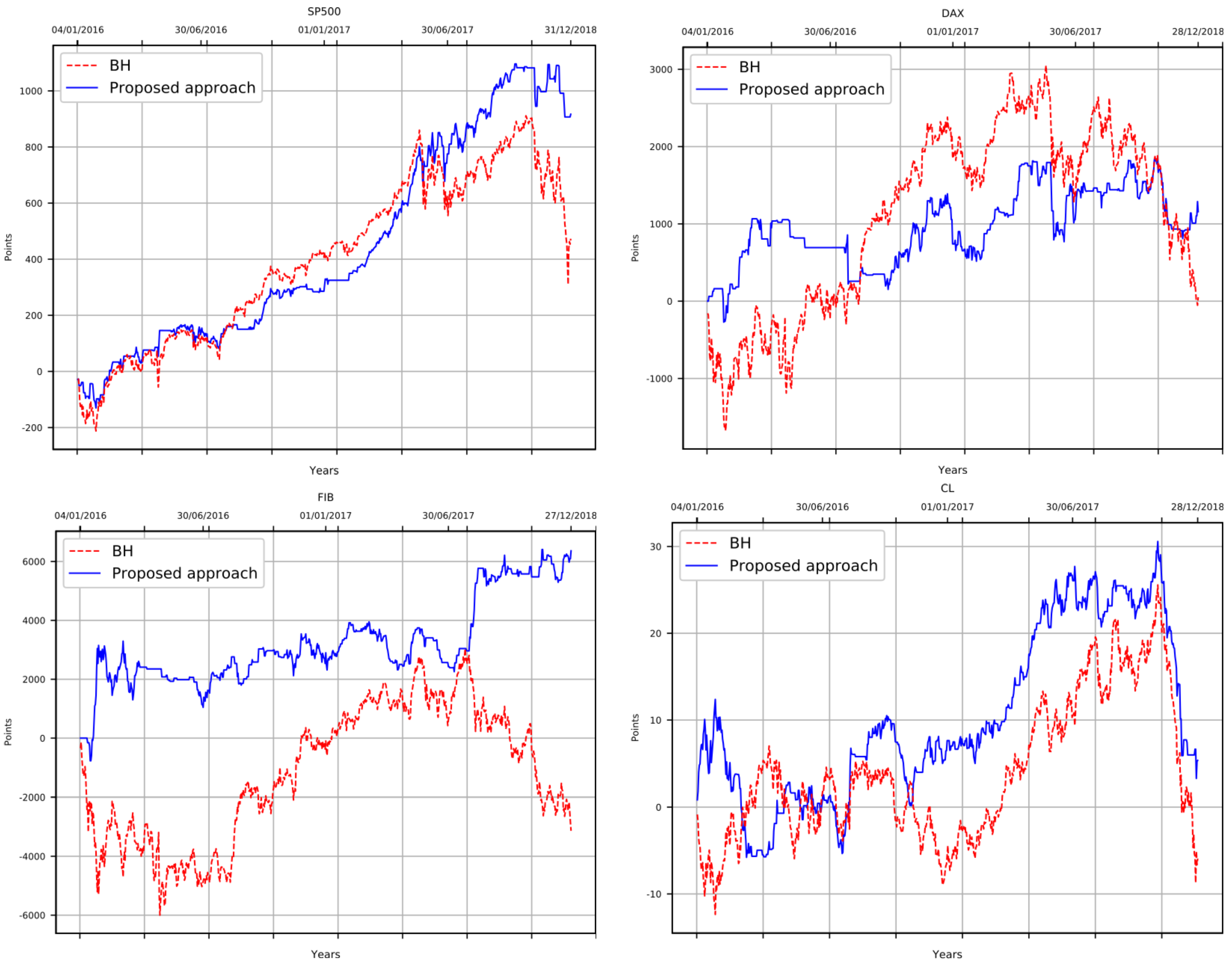
On the basis of the aforementioned considerations, Figure 2 shows the equity curves for the considered markets. As far as our ensemble approach is concerned, results and discussions are consistent with those in Table 8, whereas Buy and Hold results and discussions are consistent with Table 6 or Table 7. The difference is that the equity curve indicates the cumulative return of the underlying market within the considered OOS test data, whereas the results of the tables indicate the final value over the entire period. As far as the DAX market is concerned, the reader may notice that, although our proposed ensemble is slightly worse than the results of the BH approach, it shows a positive return. The worse performance of our approach relies on the fact that we are maintaining the same classifiers in the ensemble, no matter the market. We envision that a further step of the proposed approach in the future is also performing a data-driven selection of classifiers in the ensemble according to the market behavior.

5.2. Performance Metrics Trade Impact

In this part of the experiments, we report the trading results of our approach against the BH benchmark when considering different performance metrics in Algorithms 1 and 2.

Table 9. Comparison of the proposed approach against the Buy and Hold benchmark by considering different performance metrics in building the proposed self-configurable ensemble.

Accuracy														Buy and Hold					Our Performance
market	year	walk	train	lags	ica	preacc	accuracy	coverage	mdd	mdd	return	return	romad	mdd	mdd	return	return	romad	mdd	return	romad
		size	(%)		comp					(%)		(%)			(%)		(%)		(%)	(%)
SP500	2016–2018	100	65	9	5	0.54	0.57	0.63	406.5	19.95	485.75	23.84	1.19	601.75	29.53	473	23.21	0.79	+	+	+
DAX	2016–2018	300	65	7	0	0.53	0.52	0.55	2184.5	20.77	9.5	0.09	0	3102.5	29.49	51.5	0.49	0.02	+
CL	2016–2018	200	80	7	5	0.5	0.55	0.57	17.56	33.65	13.19	25.28	0.75	34.29	65.71	−5.92	−11.35	−0.17	+	+	+
FIB	2016–2018	250	65	1	5	0.5	0.52	0.42	1655	7.84	2760	13.07	1.67	6175	29.25	−3135	−14.85	−0.51	+	+	+
Return														Buy and Hold					Our Performance
market	year	walk	train	lags	ica	preacc	accuracy	coverage	mdd	mdd	return	return	romad	mdd	mdd	return	return	romad	mdd	return	romad
		size	(%)		comp					(%)		(%)			(%)		(%)		(%)	(%)
SP500	2016–2018	300	80	1	3	0.57	0.55	0.54	452.25	22.19	220.5	10.82	0.49	601.75	29.53	473	23.21	0.79	+
DAX	2016–2018	300	70	3	5	0.55	0.52	0.6	2732	25.97	106	1.01	0.04	3102.5	29.49	51.5	0.49	0.02	+	+	+
CL	2016–2018	250	80	3	5	0.51	0.54	0.55	29.87	57.24	−10.09	−19.34	−0.34	34.29	65.71	−5.92	−11.35	−0.17	+
FIB	2016–2018	100	80	7	2	0.51	0.52	0.47	2495	11.82	4485	21.25	1.8	6175	29.25	−3135	−14.85	−0.51	+	+	+
RoMaD														Buy and Hold					Our Performance
market	year	walk	train	lags	ica	preacc	accuracy	coverage	mdd	mdd	return	return	romad	mdd	mdd	return	return	romad	mdd	return	romad
		size	(%)		comp					(%)		(%)			(%)		(%)		(%)	(%)
SP500	2016–2018	200	80	5	5	0.53	0.57	0.68	365.25	17.92	320.5	15.73	0.88	601.75	29.53	473	23.21	0.79	+		+
DAX	2016–2018	200	60	9	5	0.52	0.56	0.42	972	9.24	2400	22.81	2.47	3102.5	29.49	51.5	0.49	0.02	+	+	+
CL	2016–2018	250	80	3	5	0.51	0.54	0.55	29.87	57.24	−10.09	−19.34	−0.34	34.29	65.71	−5.92	−11.35	−0.17	+
FIB	2016–2018	150	70	3	5	0.49	0.49	0.48	6975	33.04	−5930	−28.09	−0.85	6175	29.25	−3135	−14.85	−0.51
Return (%)														Buy and Hold					Our Performance
market	year	walk	train	lags	ica	preacc	accuracy	coverage	mdd	mdd	return	return	romad	mdd	mdd	return	return	romad	mdd	return	romad
		size	(%)		comp					(%)		(%)			(%)		(%)		(%)	(%)
SP500	2016–2018	300	80	1	3	0.57	0.55	0.54	452.25	22.19	220.5	10.82	0.49	601.75	29.53	473	23.21	0.79	+
DAX	2016–2018	300	70	3	5	0.55	0.52	0.6	2732	25.97	106	1.01	0.04	3102.5	29.49	51.5	0.49	0.02	+	+	+
CL	2016–2018	250	80	3	5	0.51	0.54	0.55	29.87	57.24	−10.09	−19.34	−0.34	34.29	65.71	−5.92	−11.35	−0.17	+
FIB	2016–2018	100	80	7	2	0.51	0.52	0.47	2495	11.82	4485	21.25	1.8	6175	29.25	−3135	−14.85	−0.51	+	+	+
MDD (%)														Buy and Hold					Our Performance
market	year	walk	train	lags	ica	preacc	accuracy	coverage	mdd	mdd	return	return	romad	mdd	mdd	return	return	romad	mdd	return	romad
		size	(%)		comp					(%)		(%)			(%)		(%)		(%)	(%)
SP500	2016–2018	250	65	9	2	0.54	0.56	0.56	315.25	15.47	156.5	7.68	0.5	601.75	29.53	473	23.21	0.79	+
DAX	2016–2018	150	65	1	4	0.5	0.53	0.5	3202	30.44	−2368.5	−22.52	−0.74	3102.5	29.49	51.5	0.49	0.02
CL	2016–2018	250	65	5	2	0.49	0.51	0.53	24.11	46.21	−5.47	−10.48	−0.23	34.29	65.71	−5.92	−11.35	−0.17	+	+
FIB	2016–2018	200	80	3	0	0.49	0.47	0.41	5653	26.78	−3753	−17.78	−0.66	6175	29.25	−3135	−14.85	−0.51	+

shows the results, where we indicate, for each market, the best hyperparameters found for the ensemble (in blue), classification metrics (in white) and risk and financial metrics (in green), together with BH metrics for the same markets (in gray). With such a study, we investigate what is the best metric to consider when optimizing the intra and hyper parameters of the proposed approach.

It can be seen from Table 9 that, for accuracy and return performance metrics, the risk is decreased (better MDD) no matter the market used. However, the accuracy proved to be the best metric as we have four better MDD metrics, three better returns, and three better RoMads, totalling ten wins against two losses from BH. All the other metrics do not beat the BH more than the accuracy, but the results in this table show that there is a correlation between high accuracy in the training of the ensemble and a low risk in the trading real-world environment. This can be particularly noted from the results in Table 8, where our proposed approach proved to be the only one who obtained positive returns in all the markets. A solution like the proposed ensemble can be a good solution for initial investors who want a trade-off between low risk and non-negative returns. This is explained because an ensemble does not trade all the time (low coverage), so a better accuracy in these less frequent trading times makes a more efficient and less risky trading system. These results are therefore further evidence of the goodness and robustness of the proposed approach, especially in the presence of atypical and unpredictable markets.

6. Conclusions

The high degree of complexity, dynamism, and the non-stationary nature of data involved in the futures markets makes the definition of an effective prediction model a challenge. In order to face this problem, this paper introduced an auto-configurable ensemble approach to significantly improve the performance of trading. This is done through optimizing two sets of parameters in late and early past data, returning customized ensembles that act by a complete agreement strategy in any kind of market.

By following a methodological experimental approach, our proposed automatic ensemble method starts auto-tuning hyper parameters in late past data. Among these hyperparameters, we tune feature selection parameters, which will return the best possible inputs for each classifier in the ensemble and also time series parameters, which will present the best disposal of features for the classifiers. As the last step, we tuned intrinsic classifiers parameters, creating powerful ensembles with classifiers trained with recent past data. Such an automatic ensemble fine-tune model returns an ensemble of best possible individual classifiers found in the training data, which can be applied for different markets. All these parameters optimizations are done through a Walk Forward Optimization approach considering the non-anchored modality. Results of trading in an out-of-sample data, spanning years 2016, 2017, and 2018 show that, despite the data complexity, the proposed ensemble model is able to get good performance in the context of positive returns in all the markets taken into consideration, being a good strategy for conservative investors who want to diversify, but keeping their investments profitable. It also turned out that, in one market, the proposed approach fails at achieving better trading performance than baselines. We believe that, in addition to select ad hoc hyper-parameters and intra-parameters for each market, an automatic selection of new ad hoc classifiers to be used by our proposed approach must also be done. We believe that this additional step can find new classifiers useful to understand different natures of data from different markets.

As future works for this research, a straightforward direction in which we are already heading lies within the domain of the Deep Learning ensembles. In fact, we are currently developing different models of deep neural networks, with the aim of creating an ensemble of them and testing them on the same out of sample markets data. Additionally, the investigation of other feature selection optimizations and even the creation of an ad hoc methodology is in our future research goals. One more path we are already exploring consists of applying the results of our ensemble to real trading platforms. The goal is, on the one hand, to simulate the real earnings we would have obtained on the past data and on a desired market. With the test being robust, on the other hand, the next step would be to perform real-time trading in a certain number of markets. The platform we are already playing with is MultiCharts (https://www.multicharts.com/). Moreover, one more possible future work can involve the definition of multi-markets strategies, able to improve the prediction performance by diversifying the investments or by using information about the behavior of many markets, in order to fine-tune the kind of classifiers used or their predictions. Finally, as stated before, a data-driven selection of classifiers for the ensemble, rather than just intrinsic and hyper parameters, is a promising research direction to be done.

References

- Cavalcante, R.C.; Brasileiro, R.C.; Souza, V.L.F.; Nóbrega, J.P.; Oliveira, A.L.I. Computational Intelligence and Financial Markets: A Survey and Future Directions. Expert Syst. Appl. 2016, 55, 194–211. [Google Scholar] [CrossRef]
- Preethi, G.; Santhi, B. Stock market forecasting techniques: A survey. J. Theor. Appl. Inf. Tech. 2012, 46. [Google Scholar]
- Patel, J.; Shah, S.; Thakkar, P.; Kotecha, K. Predicting stock and stock price index movement using trend deterministic data preparation and machine learning techniques. Expert Syst. Appl. 2015, 42, 259–268. [Google Scholar] [CrossRef]
- Ding, X.; Zhang, Y.; Liu, T.; Duan, J. Deep learning for event-driven stock prediction. In Proceedings of the Twenty-Fourth International Joint Conference on Artificial Intelligence, Buenos Aires, Argentina, 25–31 July 2015. [Google Scholar]
- Nguyen, T.H.; Shirai, K. Topic modeling based sentiment analysis on social media for stock market prediction. In Proceedings of the 53rd Annual Meeting of the Association for Computational Linguistics and the 7th International Joint Conference on Natural Language Processing, Beijing, China, 26–31 July 2015. [Google Scholar]
- Bollen, J.; Mao, H.; Zeng, X. Twitter mood predicts the stock market. J. Comput. Sci. 2011, 2, 1–8. [Google Scholar] [CrossRef]
- Rao, T.; Srivastava, S. Analyzing stock market movements using twitter sentiment analysis. In Proceedings of the 2012 International Conference on Advances in Social Networks Analysis and Mining (ASONAM 2012), Istanbul, Turkey, 26–29 August 2012. [Google Scholar]
- Carta, S.; Corriga, A.; Mulas, R.; Recupero, D.R.; Saia, R. A Supervised Multi-class Multi-label Word Embeddings Approach for Toxic Comment Classification. In Proceedings of the 11th International Joint Conference on Knowledge Discovery, Knowledge Engineering and Knowledge Management, Vienna, Austria, 17–19 September 2019. [Google Scholar]
- Oberlechner, T. Importance of technical and fundamental analysis in the European foreign exchange market. Int. J. Finance Econ. 2001, 6, 81–93. [Google Scholar] [CrossRef]
- Roberts, H.V. Stock-Market “Patterns” In addition, Financial Analysis: Methodological Suggestions. J. Finance 1959, 14, 1–10. [Google Scholar]
- Weigend, A.S. Time Series Prediction: Forecasting the Future and Understanding the Past; Addison-Wesley: Boston, MA, USA, 1994. [Google Scholar]
- Chatterjee, S.; Hadi, A.S. Regression Analysis by Example; John Wiley & Sons: Hoboken, NJ, USA, 2015. [Google Scholar]
- Misra, P.; Siddharth, L. Machine learning and time series: Real world applications. In Proceedings of the 2017 IEEE International Conference on Computing, Communication and Automation (ICCCA), Greater Noida, India, 5–6 May 2017. [Google Scholar]
- Ince, H.; Trafalis, T.B. A hybrid forecasting model for stock market prediction. Econ. Comput. Econ. Cybernetics Stud. Res. 2017, 51, 263–280. [Google Scholar]
- Teixeira, L.A.; De Oliveira, A.L.I. A method for automatic stock trading combining technical analysis and nearest neighbor classification. Expert Syst. Appl. 2010, 37, 6885–6890. [Google Scholar] [CrossRef]
- Upadhyay, V.P.; Panwar, S.; Merugu, R.; Panchariya, R. Forecasting stock market movements using various kernel functions in support vector machine. In Proceedings of the International Conference on Advances in Information Communication Technology & Computing, Bikaner, India, 12–13 August 2016. [Google Scholar]
- Zhang, Y.; Wu, L. Stock market prediction of S&P 500 via combination of improved BCO approach and BP neural network. Expert Syst. Appl. 2009, 36, 8849–8854. [Google Scholar]
- Hafezi, R.; Shahrabi, J.; Hadavandi, E. A bat-neural network multi-agent system (BNNMAS) for stock price prediction: Case study of DAX stock price. Appl. Soft Comput. 2015, 29, 196–210. [Google Scholar] [CrossRef]
- Chowdhury, U.N.; Chakravarty, S.K.; Hossain, M.T. Short-Term Financial Time Series Forecasting Integrating Principal Component Analysis and Independent Component Analysis with Support Vector Regression. J. Comput. Commun. 2018, 6, 51. [Google Scholar] [CrossRef]
- Vanstone, B.; Finnie, G. An empirical methodology for developing stockmarket trading systems using artificial neural networks. Expert Syst. Appl. 2009, 36, 6668–6680. [Google Scholar] [CrossRef]
- Rollinger, T.; Hoffman, S. Sortino ratio: A better measure of risk. Futures Mag. 2013, 1, 40–42. [Google Scholar]
- White, J.; Haghani, V. A Brief History of Sharpe Ratio, and Beyond. Available online: https://papers.ssrn.com/sol3/papers.cfm?abstract_id=3077552 (accessed on 19 November 2019).
- Frugier, A. Returns, volatility and investor sentiment: Evidence from European stock markets. Res. Int. Bus. Finance 2016, 38, 45–55. [Google Scholar] [CrossRef]
- Saia, R.; Carta, S. Evaluating Credit Card Transactions in the Frequency Domain for a Proactive Fraud Detection Approach. In Proceedings of the 14th International Joint Conference on e-Business and Telecommunications (ICETE 2017), Madrid, Spain, 24–26 July 2017. [Google Scholar]
- Saia, R.; Carta, S. A Frequency-domain-based Pattern Mining for Credit Card Fraud Detection. In Proceedings of the 2nd International Conference on Internet of Things, Big Data and Security, Porto, Portugal, 24–26 April 2017. [Google Scholar]
- Saia, R. A Discrete Wavelet Transform Approach to Fraud Detection. In Proceedings of the 11th International Conference on Network and System Security, Helsinki, Finland, 21–23 August 2017. [Google Scholar]
- Weng, H.; Li, Z.; Ji, S.; Chu, C.; Lu, H.; Du, T.; He, Q. Online e-commerce fraud: A large-scale detection and analysis. In Proceedings of the 2018 IEEE 34th International Conference on Data Engineering (ICDE), Paris, France, 16–19 April 2018. [Google Scholar]
- Saia, R.; Carta, S. Evaluating the benefits of using proactive transformed-domain-based techniques in fraud detection tasks. Future Generation Comp. Syst. 2019, 93, 18–32. [Google Scholar] [CrossRef]
- Saia, R.; Boratto, L.; Carta, S. Multiple Behavioral Models: A Divide and Conquer Strategy to Fraud Detection in Financial Data Streams. In Proceedings of the 2015 7th International Joint Conference on Knowledge Discovery, Knowledge Engineering and Knowledge Management (IC3K), Lisbon, Portugal, 12–14 November 2015. [Google Scholar]
- Chatfield, C. The Analysis of Time Series: An Introduction; CRC Press: Boca Raton, FL, USA, 2016. [Google Scholar]
- Trippi, R.R.; Turban, E. Neural Networks in Finance and Investing: Using Artificial Intelligence to Improve Real World Performance; McGraw-Hill, Inc.: Boston, MA, USA, 1992. [Google Scholar]
- Kara, Y.; Boyacioglu, M.A.; Baykan, Ö.K. Predicting direction of stock price index movement using artificial neural networks and support vector machines: The sample of the Istanbul Stock Exchange. Expert Syst. Appl. 2011, 38, 5311–5319. [Google Scholar] [CrossRef]
- Wu, Y.; Mao, J.; Li, W. Predication of Futures Market by Using Boosting Algorithm. In Proceedings of the 2018 International Conference on Wireless Communications, Signal Processing and Networking (WiSPNET), Chennai, India, 22–24 March 2018. [Google Scholar]
- Idrees, S.M.; Alam, M.A.; Agarwal, P. A Prediction Approach for Stock Market Volatility Based on Time Series Data. IEEE Access 2019, 7, 17287–17298. [Google Scholar] [CrossRef]
- Carta, S.; Medda, A.; Pili, A.; Reforgiato Recupero, D.; Saia, R. Forecasting E-Commerce Products Prices by Combining an Autoregressive Integrated Moving Average (ARIMA) Model and Google Trends Data. Future Internet 2019, 11, 5. [Google Scholar] [CrossRef]
- Weerathunga, H.P.S.D.; Silva, A.T.P. DRNN-ARIMA Approach to Short-term Trend Forecasting in Forex Market. In Proceedings of the 2018 18th International Conference on Advances in ICT for Emerging Regions (ICTer), Colombo, Sri Lanka, 26–29 September 2018. [Google Scholar]
- Chou, J.; Nguyen, T. Forward Forecast of Stock Price Using Sliding-Window Metaheuristic-Optimized Machine-Learning Regression. IEEE Trans. Ind. Inf. 2018, 14, 3132–3142. [Google Scholar] [CrossRef]
- Nobre, J.; Neves, R.F. Combining Principal Component Analysis, Discrete Wavelet Transform and XGBoost to trade in the financial markets. Expert Syst. Appl. 2019, 125, 181–194. [Google Scholar] [CrossRef]
- Gupta, D.; Pratama, M.; Ma, Z.; Li, J.; Prasad, M. Financial time series forecasting using twin support vector regression. PLoS ONE 2019, 14, e0211402. [Google Scholar] [CrossRef] [PubMed]
- Prasad, M.; Lin, Y.; Lin, C.; Er, M.; Prasad, O. A new data-driven neural fuzzy system with collaborative fuzzy clustering mechanism. Neurocomputing 2015, 167, 558–568. [Google Scholar] [CrossRef]
- Patel, O.P.; Bharill, N.; Tiwari, A.; Prasad, M. A Novel Quantum-inspired Fuzzy Based Neural Network for Data Classification. IEEE Trans. Emerg. Topics Comput. 2019, 1–14. [Google Scholar] [CrossRef]
- Klir, G.J.; Folger, T.A. Fuzzy Sets, Uncertainty, and Information; Prentice-Hall, Inc.: Upper Saddle River, NJ, USA, 1987. [Google Scholar]
- Gonçalves, R.; Ribeiro, V.M.; Pereira, F.L.; Rocha, A.P. Deep learning in exchange markets. Inf. Econ. Policy 2019, 47, 38–51. [Google Scholar] [CrossRef]
- Chatzis, S.P.; Siakoulis, V.; Petropoulos, A.; Stavroulakis, E.; Vlachogiannakis, N. Forecasting stock market crisis events using deep and statistical machine learning techniques. Expert Syst. Appl. 2018, 112, 353–371. [Google Scholar] [CrossRef]
- Deng, Y.; Bao, F.; Kong, Y.; Ren, Z.; Dai, Q. Deep Direct Reinforcement Learning for Financial Signal Representation and Trading. IEEE Trans. Neural Netw. Learn. Syst. 2017, 28, 653–664. [Google Scholar] [CrossRef]
- Dietterich, T.G. Ensemble Methods in Machine Learning. In Proceedings of the International Workshop on Multiple Classifier Systems, Cagliari, Italy, 21–23 June 2000. [Google Scholar]
- Zainal, A.; Maarof, M.A.; Shamsuddin, S.M.H.; Abraham, A. Ensemble of One-Class Classifiers for Network Intrusion Detection System. In Proceedings of the Fourth International Conference on Information Assurance and Security (IAS), Napoli, Italy, 8–10 September 2008. [Google Scholar]
- Saia, R.; Salvatore, C.; RECUPERO, R. A Probabilistic-driven Ensemble Approach to Perform Event Classification in Intrusion Detection System. In Proceedings of the 10th International Joint Conference on Knowledge Discovery, Knowledge Engineering and Knowledge Management, Seville, Spain, 18–20 September 2018. [Google Scholar]
- Carta, S.; Fenu, G.; Recupero, D.R.; Saia, R. Fraud detection for E-commerce transactions by employing a prudential Multiple Consensus model. J. Inf. Secur. Appl. 2019, 46, 13–22. [Google Scholar] [CrossRef]
- Sagi, O.; Rokach, L. Ensemble learning: A survey. Wiley Interdiscip. Rew.: Data Min. Knowl. Discov. 2018, 8, e1249. [Google Scholar] [CrossRef]
- Zhu, B.; Ye, S.; Wang, P.; He, K.; Zhang, T.; Wei, Y.M. A novel multiscale nonlinear ensemble leaning paradigm for carbon price forecasting. Energy Econ. 2018, 70, 143–157. [Google Scholar] [CrossRef]
- Ratto, A.P.; Merello, S.; Oneto, L.; Ma, Y.; Malandri, L.; Cambria, E. Ensemble of Technical Analysis and Machine Learning for Market Trend Prediction. In Proceedings of the IEEE Symposium Series on Computational Intelligence (SSCI), Bangalore, India, 18–21 November 2018. [Google Scholar]
- Sun, S.; Sun, Y.; Wang, S.; Wei, Y. Interval decomposition ensemble approach for crude oil price forecasting. Energy Econ. 2018, 76, 274–287. [Google Scholar] [CrossRef]
- Gan, K.S.; Chin, K.O.; Anthony, P.; Chang, S.V. Homogeneous Ensemble FeedForward Neural Network in CIMB Stock Price Forecasting. In Proceedings of the International Conference on Artificial Intelligence in Engineering and Technology (IICAIET), Kota Kinabalu, Malaysia, 8 November 2018. [Google Scholar]
- Ding, Y. A novel decompose-ensemble methodology with AIC-ANN approach for crude oil forecasting. Energy 2018, 154, 328–336. [Google Scholar] [CrossRef]
- Gomes, H.M.; Barddal, J.P.; Enembreck, F.; Bifet, A. A Survey on Ensemble Learning for Data Stream Classification. ACM Comput. Surv. 2017, 50. [Google Scholar] [CrossRef]
- Choi, S. Independent component analysis. In Encyclopedia of Biometrics; Springer: New York, NY, USA, 2015; pp. 917–924. [Google Scholar]
- Hyvärinen, A.; Oja, E. Independent component analysis: Algorithms and applications. Neural Netw. 2000, 13, 411–430. [Google Scholar] [CrossRef]
- Jutten, C.; Karhunen, J. Advances in blind source separation (BSS) and independent component analysis (ICA) for nonlinear mixtures. Int. J. Neural Syst. 2004, 14, 267–292. [Google Scholar] [CrossRef] [PubMed]
- Jutten, C.; Herault, J. Blind separation of sources, part I: An adaptive algorithm based on neuromimetic architecture. Signal Process. 1991, 24, 1–10. [Google Scholar] [CrossRef]
- Huang, W.; Nakamori, Y.; Wang, S.Y. Forecasting stock market movement direction with support vector machine. Comput. Operat. Res. 2005, 32, 2513–2522. [Google Scholar] [CrossRef]
- Döpke, J.; Fritsche, U.; Pierdzioch, C. Predicting recessions with boosted regression trees. Int. J. Forecast. 2017, 33, 745–759. [Google Scholar] [CrossRef]
- Kirkpatrick, C.D.; Dahlquist, J.R. Technical Analysis: The Complete Resource for Financial Market Technicians; FT Press Science: Upper Saddle River, NJ, USA, 2010. [Google Scholar]
- Tomasini, E.; Jaekle, U. Trading Systems; Harriman House Limited: Petersfield, UK, 2011. [Google Scholar]
- Sharkey, A.J.C. On combining artificial neural nets. Connect. Sci. 1996, 8, 299–314. [Google Scholar] [CrossRef]
- Tsymbal, A.; Pechenizkiy, M.; Cunningham, P. Diversity in search strategies for ensemble feature selection. Inf. Fusion 2005, 6, 83–98. [Google Scholar] [CrossRef]
- Van Wezel, M.; Potharst, R. Improved customer choice predictions using ensemble methods. Eur. J. Operat. Res. 2007, 181, 436–452. [Google Scholar] [CrossRef] [Green Version]
- Magdon-Ismail, M.; Atiya, A.F. Maximum drawdown. Risk Mag. 2004, 17, 99–102. [Google Scholar]
- Hayes, R.M. The impact of trading commission incentives on analysts’ stock coverage decisions and earnings forecasts. J. Account. Res. 1998, 36, 299–320. [Google Scholar] [CrossRef]
- Alostad, H.; Davulcu, H. Directional prediction of stock prices using breaking news on Twitter. Web Intell. 2017, 15, 1–17. [Google Scholar] [CrossRef] [Green Version]
- Alajbeg, D.; Bubaš, Z.; Ivan, Š. The P/E Effect on the Croatian Stock Market. J. Int. Sci. Publ. Econ. Bus. 2016, 10, 84. [Google Scholar]
- Schipper, K.; Smith, A. A comparison of equity carve-outs and seasoned equity offerings: Share price effects and corporate restructuring. J. Financial Econ. 1986, 15, 153–186. [Google Scholar] [CrossRef]
- Enke, D.; Grauer, M.; Mehdiyev, N. Stock market prediction with multiple regression, fuzzy type-2 clustering and neural networks. Procedia Comput. Sci. 2011, 6, 201–206. [Google Scholar] [CrossRef] [Green Version]
- Klassen, M. Investigation of Some Technical Indexes in Stock Forecasting Using Neural Networks. In Proceedings of the Third World Enformatika Conference, Istanbul, Turkey, 27–29 April 2005. [Google Scholar]
- Tetlock, P.C. Giving content to investor sentiment: The role of media in the stock market. J. Finance 2007, 62, 1139–1168. [Google Scholar] [CrossRef]
- Dean, J.; Ghemawat, S. MapReduce: Simplified data processing on large clusters. Commun. ACM 2008, 51, 107–113. [Google Scholar] [CrossRef]
- Hashem, I.A.T.; Anuar, N.B.; Gani, A.; Yaqoob, I.; Xia, F.; Khan, S.U. MapReduce: Review and open challenges. Scientometrics 2016, 109, 389–422. [Google Scholar] [CrossRef]
Figure 1.
The proposed two-step auto adjustable parameters ensemble for market forecasting. This approach optimizes two sets of parameters for a final ensemble to trade in any market. Firstly, in an in-sample dataset with late past data, we optimize the hyperparameters, considering performance metrics in the testing part of data. Then, these hyperparameters are transferred to create ensembles for an early past (out of sample) dataset. The individual classifiers have their intrinsic parameters updated in the validation part of this recent data and then the final ensemble is built.
Figure 2.
Equity curves.