An Efficient Two-Layer Non-Hydrostatic Model for Investigating Wave Run-Up Phenomena


Faculty of Mathematics and Natural Sciences, Bandung Institute of Technology, Bandung 40132, Indonesia
*
Author to whom correspondence should be addressed.
Computation 2020, 8(1), 1; https://0-doi-org.brum.beds.ac.uk/10.3390/computation8010001
Submission received: 28 October 2019
/
Revised: 23 December 2019
/
Accepted: 24 December 2019
/
Published: 27 December 2019
(This article belongs to the Section Computational Engineering)
Abstract
:In this paper, we study the maximum run-up of solitary waves on a sloping beach and over a reef through a non-hydrostatic model. We do a modification on the non-hydrostatic model derived by Stelling and Zijlema. The model is approximated by resolving the vertical fluid depth into two-layer system. In contrast to the two-layer model proposed by Stelling, here, we have a block of a tridiagonal matrix for the hydrodynamic pressure. The equations are then solved by applying a staggered finite volume method with predictor-corrector step. For validation, several test cases are presented. The first test is simulating the propagation of solitary waves over a flat bottom. Good results in amplitude and shape preservation are obtained. Furthermore, run-up simulations are conducted for solitary waves climbing up a sloping beach, following the experimental set-up by Synolakis. In this case, two simulations are performed with solitary waves of small and large amplitude. Again, good agreements are obtained, especially for the prediction of run-up height. Moreover, we validate our numerical scheme for wave run-up simulation over a reef, and the result confirms the experimental data.
1. Introduction
Wave run-up is the maximum vertical limit of wave upsurge which occurs on a beach or structure above the still water level. In the tsunami mitigation plan, a good estimation of wave run-up is needed to determine the evacuation area to protect people from the tsunami. Many researchers developed empirical formulas to predict the run-up for regular waves [1,2,3]. Analytical formulation of wave run-up was also derived for different types of incident waves based on Carrier and Greenspan’s solution [4,5,6]. Both empirical and analytical formulas are useful for practical application but they are generally limited to a simplified sloping structure. For more complex topography and general type of waves, the numerical approach is necessary to predict the wave run-up.
Several wave models can be used to approximate the wave run-up. Shallow water equations are often used in wave run-up models, especially in tsunami cases. The numerical scheme based on shallow water equations is good enough to simulate wave run-up for long waves [7,8]. However, for dispersive waves, i.e., solitary waves, this model failed to simulate the propagation with the correct speed. Thus, another model is needed in dispersive wave modelling.
There are two approaches to model the dispersive waves, i.e., Boussinesq-type and non-hydrostatic approaches. The Boussinesq-type model was constructed for irrotational and incompressible fluid flow without friction [9,10,11]. Nevertheless, the difficulty in dealing with the Boussinesq model is due to the complexity of non-linearity and dispersion terms. An alternative model that involves non-linearity and dispersion is the depth integrated non-hydrostatic model which was firstly developed by [12] to solve Euler equations with total pressure. Then, this total pressure was separated by [13] and [14] into hydrostatic and hydrodynamic pressure to improve the efficiency of the computational time.
Stelling and Zijlema (2003) [15] in SWASH and Magdalena [16] proposed an alternate depth-integrated formulation, which introduces non-hydrostatic pressure and vertical velocity terms in the non-linear shallow water equations (NSWE) to describe weakly dispersive waves. The paper presents some validations of the scheme by making a comparison between the numerical results and analytical solution, also with the experimental data. To obtain a good agreement with both analytical and experimental results, it is necessary to use two or more layers. Based on the scheme introduced by Stelling and Zijlema (2003), we propose a modification of two-layer non-hydrostatic approach.
Here, we study the performance of the modified two-layer scheme. It can handle wave frequency correctly including short waves up to kd ≈ 6. For the application of two-layer fluid system, this scheme can simulate soliton propagation with undisturbed shape. Therefore, we can conclude that the modified two-layer scheme can balance the non-linearity and dispersion effects. This is the most important test case for non-linear and dispersive model. In this research, first, we construct a momentum conservative numerical scheme without considering the dispersion effect using a staggered finite volume method. This method, which was initially investigated by [17] to solve differential equations, was further extended and implemented by many researchers [15,18,19]. Working with a staggered finite volume gives us more advantages than working in a collocated grid because we do not end up with the Riemann problem that is relatively difficult to solve, as seen in the NHWAVE proposed by [20]. Besides, this scheme could give accurate result for subcritical flow [21] and relatively simple even for three-dimensional extent [14,22,23]. Secondly, to derive the model with dispersion, we propose a non-hydrostatic approach that incorporates hydrodynamic pressure. By taking the hydrodynamic pressure into account, we consider inhomogeneity in vertical direction. This two-layer approach has a tridiagonal matrix for pressure, whereas the standard two-layer approach in SWASH by Stelling and Zijlema (2003) has a pentadiagonal matrix. Dealing with a tridiagonal matrix allows us to implement the Thomas algorithm, which is faster than a pentadiagonal matrix that needs to be solved using an iterative method. Thus, the computational cost of this two-layer approach is comparable with that of the one-layer approach [24], but the performance is comparable with the two-layer approach as conducted in Stelling and Zijlema (2003). We can argue that this two-layer approach is efficient.
In this paper, we will see how wide the range of problems that can be covered by the numerical scheme is. A series of test cases will be conducted to validate and verify the two-layer non-hydrostatic numerical scheme. First, we will simulate the propagation of solitary waves over a flat bottom topography. Then, the topography will be extended to a sloping beach with and without a reef. The results will be compared to the data measured in laboratory experiments. Finally, the numerical scheme is implemented to simulate the 2004 Indian Ocean tsunami run-up on the west coast of Aceh, Indonesia.
2. The Two-Layer Non-Hydrostatic Model
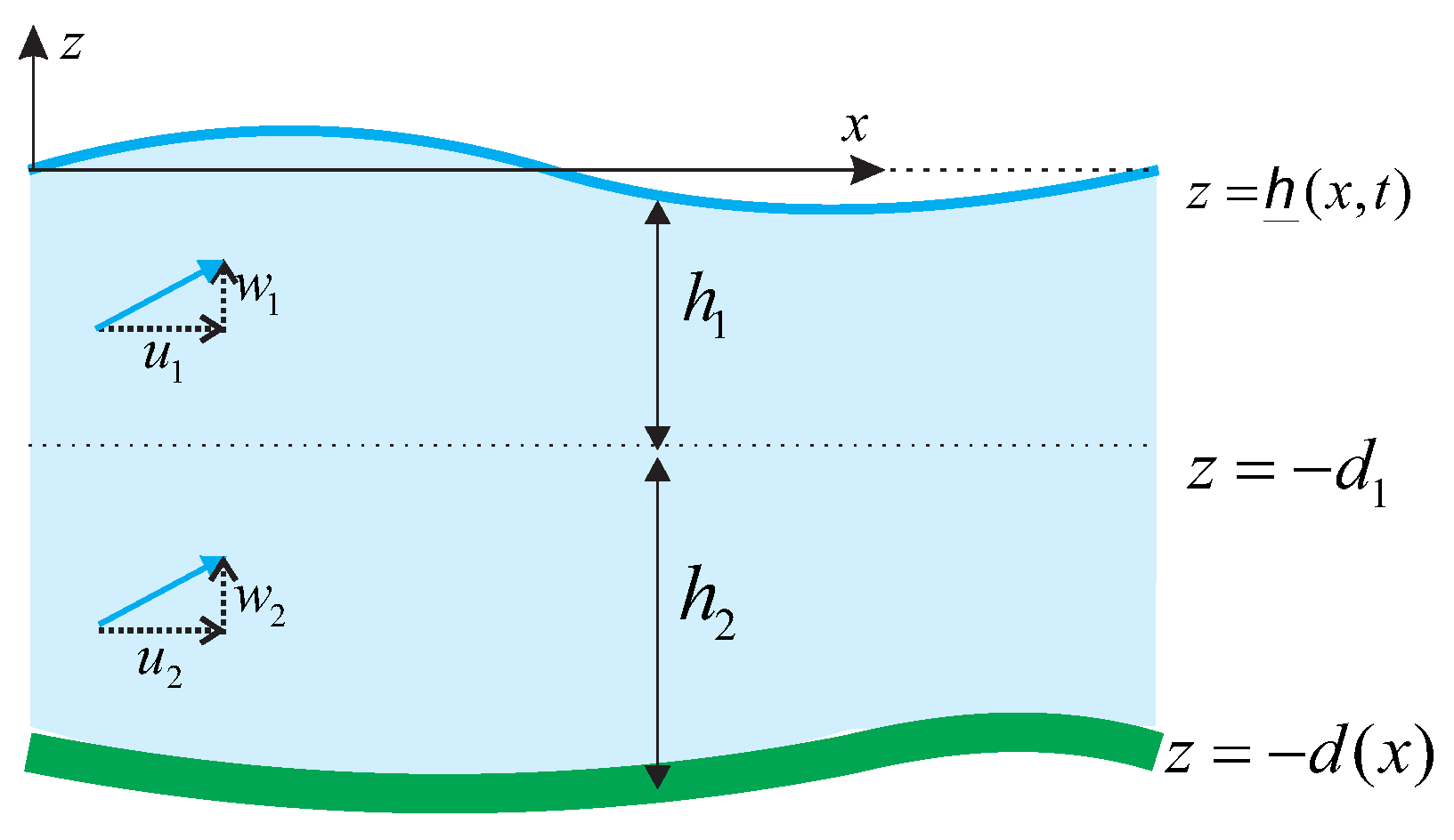
In this section, we explain briefly the derivation of the non-hydrostatic model using the two-layer approach to study wave run-up over a sloping beach. First, we consider our observation domain as a two-layer fluid system, upper and lower layer domain, that are indexed by subscript 1 and 2, respectively. The sketch of this problem is shown in Figure 1. Here, denotes the bottom topography, while denotes the free surface elevation. The interface between the two layers is located at . The water thickness for each layer is for . The horizontal and vertical velocity is denoted by and , respectively.
Our derivation based on the Euler equations model in terms of the velocity read as
where q is the essential term in this model that is our hydrodynamic pressure. Respectively, the kinematic free surface and bottom boundary conditions for the flow read as:
The subscripts and d denote the position where quantity evaluated. Based on the Euler equations above, we integrate Equations (1) and (2) from the bottom to the interface. By implementing the kinematic boundary condition (5) and Leibniz’s rule, we obtain
Similarly, for the upper layer, incorporating the kinematic boundary condition (4) and Equation (6) into the integration of Equations (1) and (2) from the interface to the surface, we obtain
Under the assumption that , then the momentum Equation (8) becomes
In this non-hydrostatic approach, vertical homogeneities are adopted. The relations between vertical velocity and hydrodynamic pressure q for the two layers come from the linearized momentum equation with the Keller-box scheme read as
The closure relations needed to calculate and come from the mass conservation for both layers as follows.
To eliminate the vertical velocity and the pressure at the bottom from the set of equations, first, Equation (12) is multiplied by 2, then added to Equation (13):
From now on, we treat as a new variable.
Here, we assume the fluid density profile increases with depth only in the upper part of a fluid column. In the lower part, fluid density value is nearly constant, as commonly observed in nature. Therefore, the hydrodynamic pressure q is assumed to be a constant function throughout the lower layer. In this two-layer formulation, we denote , so that Equation (7) is simplified to
Finally, the full set of non-hydrostatic model using two-layer approach is
The system consists of five equations with five unknown variables , and . This gives us an advantage in the computation where we do not need to compute Equation (11) anymore.
3. Dispersion Relation
In this section, we derive the dispersion relation of our linearized two-layer non-hydrostatic model over a constant depth where and . To derive the dispersion relation of the proposed model, first, we assume that the wave is a periodic wave with a small amplitude in the form of
Notation denotes wave celerity, and k is the wavenumber. Substituting Equations (21)–(25) into the linearized governing equations written as
we obtain the following dispersion relation,
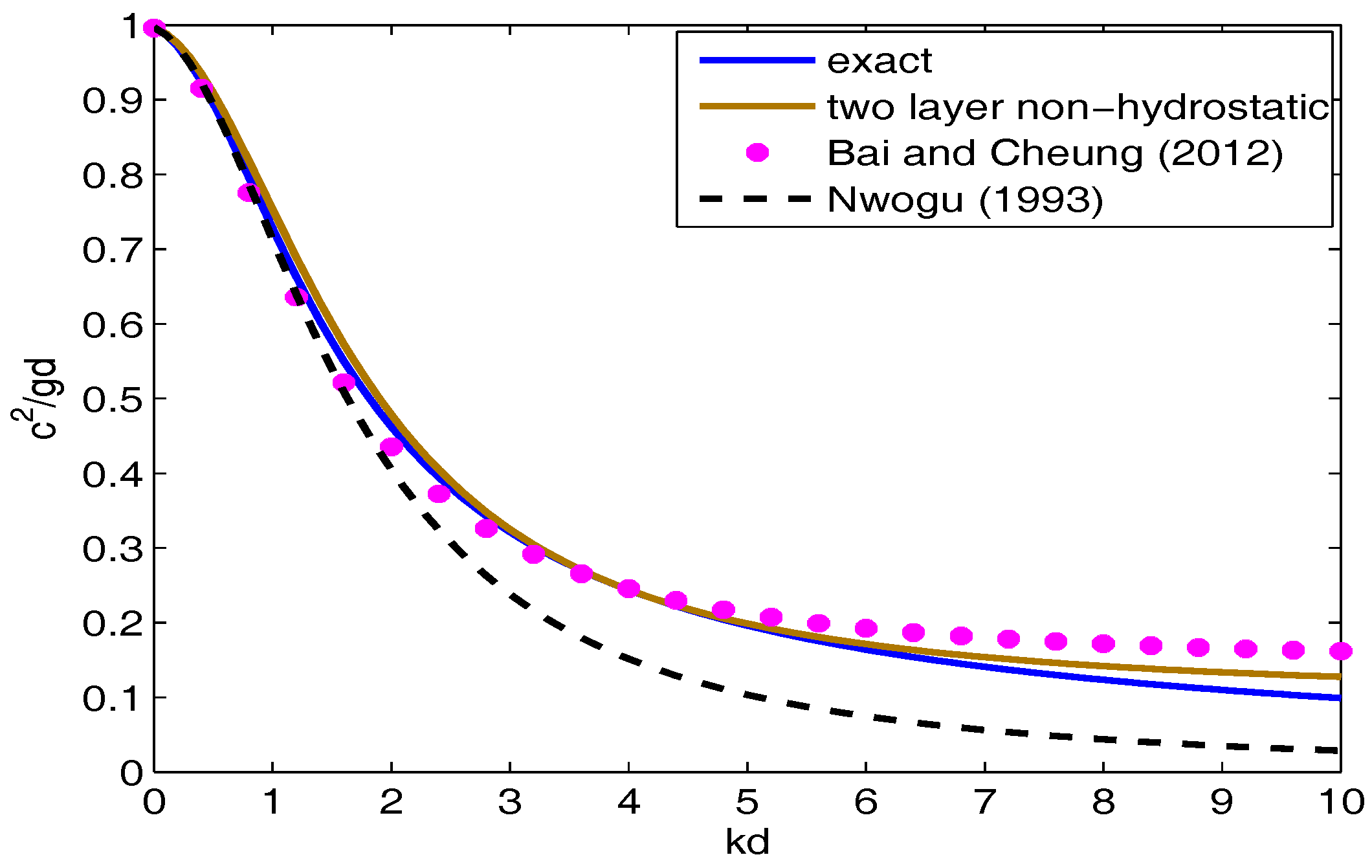
To check the accuracy of our dispersion relation, we compare it with the dispersion relation proposed by [10] and [25]. Nwogu [10] obtained the dispersion relation of Boussinesq-type model written as
where is a parameter that was adjusted to be equal to −1/3 in order to get the result closer to the exact dispersion relation. The linear dispersion relation of the hybrid system obtained by Bai and Cheung wrote as
where is a free parameter.
For the comparison between the exact dispersion relation with the ones obtained using our non-hydrostatic model, Boussinesq-type model in [10] and hybrid system in [25], we use and . The comparison is shown in Figure 2. The figure shows that our numerical dispersion relation is in a good agreement with the exact solution. Moreover, the accuracy of our result is up to with 1% error.
4. Numerical Formulation
In this section, we implement a staggered finite volume method with predictor-corrector step to solve our governing equations numerically. The predictor step is used to calculate the governing equations with neglecting the hydrodynamic pressure term. In the next step, we correct the velocity by including hydrodynamic pressure and considering inhomogeneity in the vertical direction. We use all values in the hydrostatic part as the predictor in the correction step.
4.1. Predictor Part
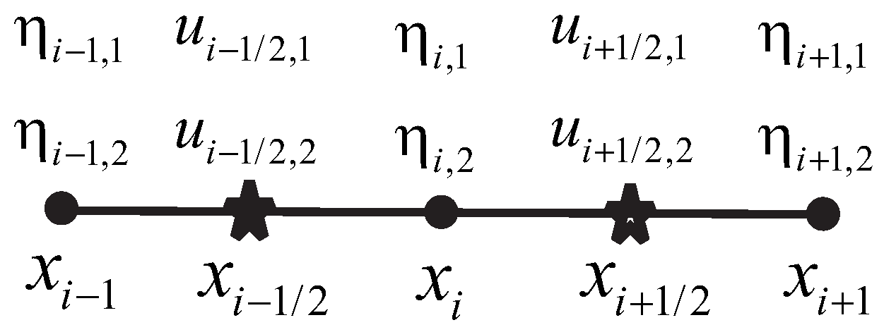
Following the staggered momentum conservative scheme for the NSWE [18,19], here, we implement the analogous scheme for our non-hydrostatic model. Consider an observation domain . Applying a staggered partition, then our grid points are , . The rules of implementing staggered arrangement, the values of are computed using mass conservation (26) at every full grid points , with . Whereas velocities are computed using momentum equation ((27), (28)) at every staggered grid points , with , see Figure 3. Since , and are functions of x, once , and are known, , and can be obtained.
Then, the approximated Equations of (26)–(28) are:
where the asterisk denotes the unknown values that we need to approximate. To estimate the values of water depth , for at half grid points, we use first order upwind method read as:
The discretization of the advection term written as
whereas
with the following upwind approximation of for both layers ,
4.2. Corrector Part
In this step, we correct the values of , and by including the hydrodynamic pressure term in the model. The staggered grid arrangement of the new calculated variables is depicted in Figure 4. The pressure variable q and vertical velocities and are calculated at the full grid points. Here, we consider the values of , and that we have obtained from the hydrostatic model as the predictor values. Those are denoted by superscript *. Taking the assumption that hydrodynamic pressure is zero at the surface, and it is constant throughout the lower layer, we only need one vector array to store q values. It is less complicated compared to the two-layer approach proposed by [26], where two vector arrays for q are needed.
In this non-hydrostatic step, we begin with Equation (20) and its discrete form which is
We substitute the values of and in the correction step that are given by:
to get a tridiagonal system of equations for . Then, we solve the tridiagonal system by means of Thomas Algorithm.
Related to [15,22,25,26]’s work, the performance of our scheme is comparable to the two-layer approach conducted by [15] with the computational cost is more efficient and comparable with one-layer approximation of [15]. In the standard two-layer approach, we have a pentadiagonal matrix, and here we have a tridiagonal matrix. In comparison, solving a standard 6 x 6 matrix with pentadiagonal linear system in MATLAB with a processor Intel(R) Core(TM) i7-8565U CPU @1.80GHz 1.99GHz will take 0.002561 seconds, and for the tridiagonal system, we only need 0.000835 seconds. Therefore, we can conclude that our numerical scheme is more efficient than the two-layer approach proposed by [15].
5. Numerical Simulations
From the previous section, we achieve the dispersion relation of the two-layer non-hydrostatic model and it gives us a good sign that our model is able to simulate non-linear and dispersive wave phenomena. Here, we shall present some benchmark tests to demonstrate the capability of our model in describing non-breaking and breaking waves evolution. First, we start with the numerical experiments of solitary wave propagation in a flat bottom channel. This test examines whether our numerical model has a balance between dispersion and nonlinearity or not. The second test case is a comparison between wave run-up calculation and experimental data for solitary waves run up on a sloping beach. Next, we show the capability of the proposed model with its wet-dry procedure in describing wave propagation over a dry area and holding a breaking wave by comparing the numerical results to the experimental data. This test case is also used to investigate the appearance of undular bore and its propagation, as well as wave run-up over a fringing reef. In the end, we implemented the numerical model to simulated the 2004 Indian Ocean tsunami run-up using simplified Aceh bathymetry.
5.1. Solitary Waves Propagate over a Flat Bottom
In this subsection, we present a benchmark test for solitary wave propagation over a flat bottom. This is a benchmark test for the dispersive and nonlinear waves. For computation, a channel with m long and m water depth is considered. The left and right absorbing boundaries are applied. The initial wave is located at and has the following surface profile
with , and . For numerical computation, we choose and . We compare the numerical solution to the exact solution written as:
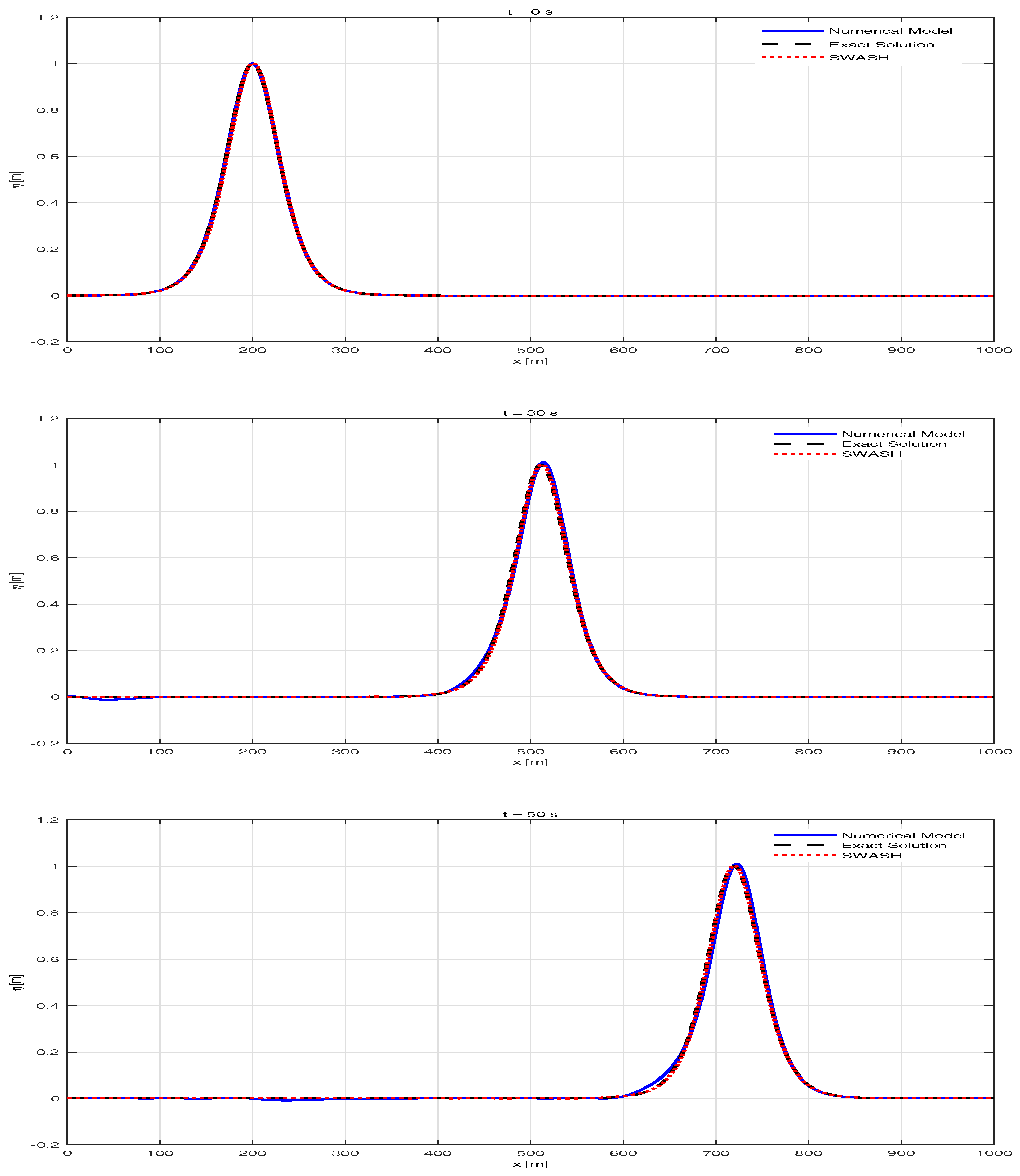
Owing to the balance between nonlinearity and dispersion, in Figure 5, we can see that the solitary waves travel with the correct speed, constant amplitude, and conserved shape. We plot the numerical result together with the analytical solution and SWASH result and they show a good comparison.
5.2. Solitary Waves Run up on a Sloping Beach
This section presents two benchmark tests to examine the profile of solitary waves propagate to a sloping area for the non-breaking and breaking case. The breaking criteria are based on the ratio of amplitude and water depth , as stated in [6], and the wave parameter for the breaking simulations is based on experimental data in that paper. The initial waves have the same profile as used in Synolakis’ experiment [6]. This experiment was conducted at 31.73 m length, 60. 96 cm depth, and 39.97 cm width wave tank. Since the length is much longer than the width, we could use this experimental data to validate a one-dimensional problem. We use a simulation set-up where the bathymetry is a flat bottom connected to a sloping beach with the beach slope is 1:19.85. The initial condition is defined in the flat bottom area as
where A is wave height, is undisturbed water depth, g is gravity acceleration, is wave crest position, and . This initial condition causes solitary waves to propagate to the beach on the right side. For this simulation, we set and . We perform two simulations which are the non-breaking case and the breaking case . We choose and to handle the moving boundary at the shoreline. In this simulation, the wet and dry procedure is applied.
We will start with a small normalized wave height . The result is summarized in Figure 6 which shows the comparison between the experimental measurements (dots), the hydrostatic model results [8] (dash line), and the two-layer non-hydrostatic model results (solid line). The comparison is noticed at four different times, at , , , and . Both of the numerical results are similar and both of them are in a good agreement with the experimental data.
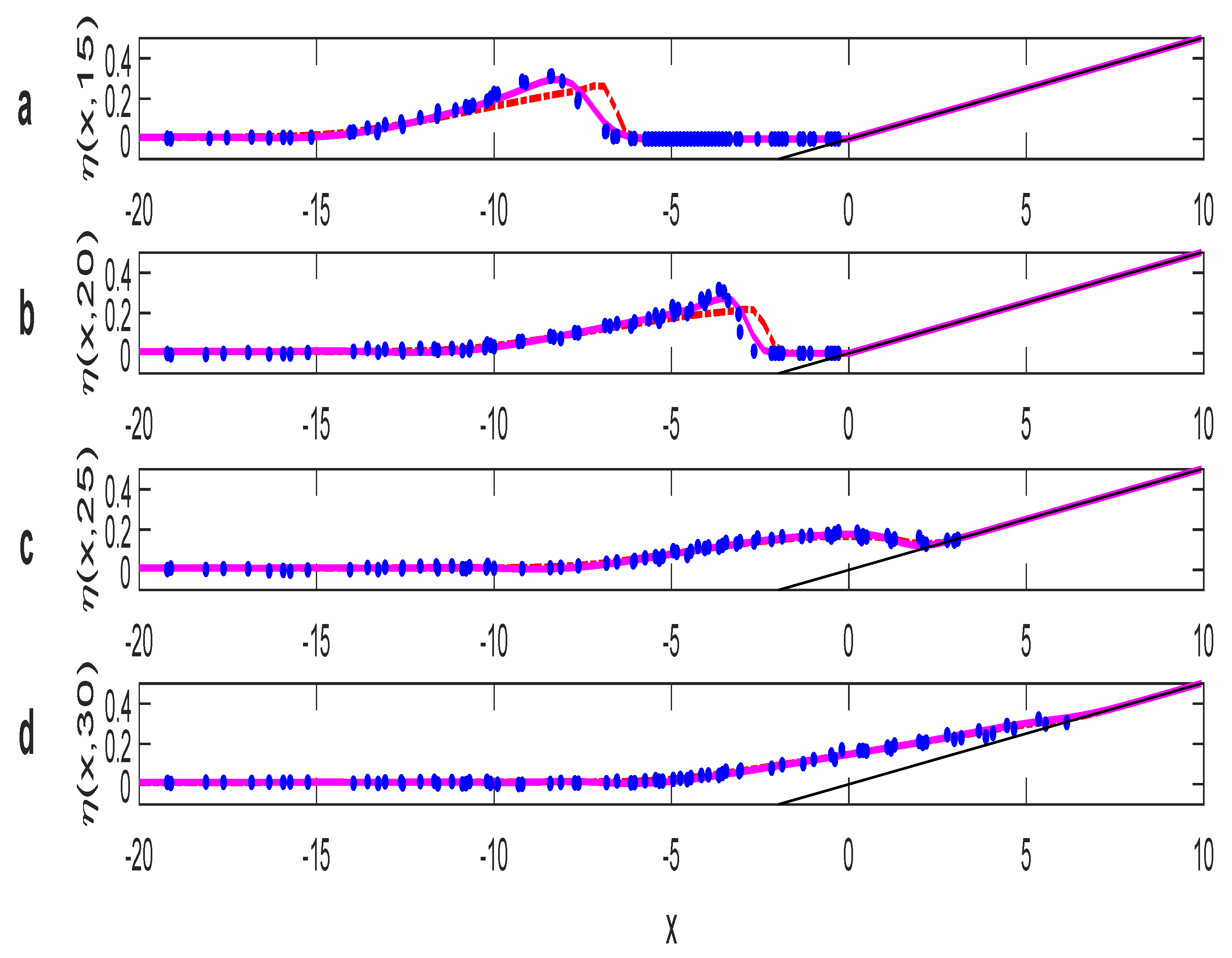
The next simulation is performed for larger normalized wave height, i.e, . Here, the surface profiles are captured at , , , and . The comparison between laboratory experiment, the hydrostatic model, and the two-layer non-hydrostatic simulation is shown in Figure 7.
As shown in Figure 7, the hydrostatic model produces wave speeds that are faster than the experiment results. Implementing the non-hydrostatic model will produce better propagation speed than the hydrostatic model. Error comparison between hydrostatic and non-hydrostatic model at and is shown in Table 1.
Next, we also compare our numerical model with BoussClaw numerical model as shown in Figure 8. BoussClaw is an extension of GeoClaw (part of Clawpack developed by LeVeque [27]) which solves the Boussinesq-type model. Both numerical models are in a good agreement with the experimental data, yet, the non-hydrostatic model produces a better approximation.
5.3. Run-up Height of Solitary Waves
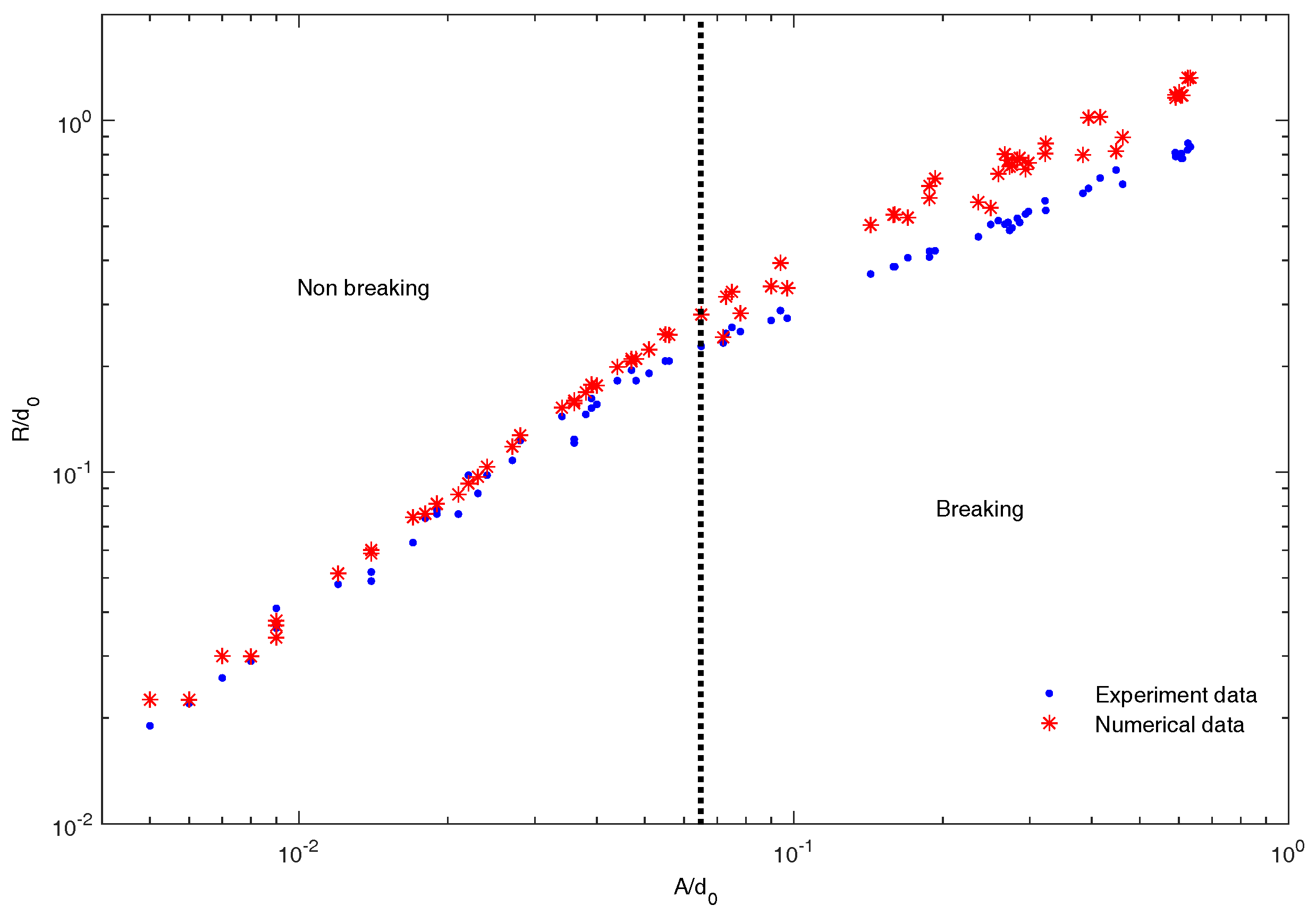
In this section, the two-layer non-hydrostatic scheme will be implemented to measure the maximum run-up of solitary waves over a sloping beach. We conduct several simulations with different depth and wave height, using the same bathymetry and initial condition as shown in the previous simulation. The value in initial condition changes with different wave height, because solitary waves with different height have different “wave length”. The value of is chosen so that the solitary hump is on the flat bottom area. In this simulation we choose as suggested by [6], where is the distance of wave crest from the toe of the beach. It is to assure that all the solitary waves propagate with the same relative distance to the beach. The experimental data in [6] were used to be compared with our model. The water depth ranged from 6.25 cm to 38.32 cm and the wave height ratio ranged from 0.005 to 0.633. As stated in [6], the wave breaks during run-up when . Run-up height for different wave height is presented in Figure 9. Compared to the experimental data, the run-up height produced by our scheme is good enough (the average error is less than 12%) for solitary waves with the non-breaking case. For solitary waves with the breaking case, run-up height that is produced by our scheme is higher than experimental data. Nevertheless, from our numerical results, we can conclude that the relative run-up height increases as the relative wave height increases, which is confirmed by the experimental data.
5.4. Solitary Waves Propagation over a Sloping Beach with Reefs
Here, we implement our numerical scheme to simulate wave run-up over a sloping beach with a fringing reef. This simulation offers a challenge for researchers who are working on numerical mathematics field because the existence of reef over a sloping beach makes the surf-zone processes more complex. The complexities are in describing the moving waterlines in the dry area and the breaking waves phenomenon. Therefore, a complete dispersive and nonlinear numerical scheme is not enough to simulate this case, so we need to include a correct wet-dry procedure.
In O.H. Hinsdale Wave Research Laboratory of Oregon State University, [28] has investigated the transformation of solitary waves over a fringing reef under wet and dry flat conditions. He has done several experiments with different set-ups. Here, we choose two set-ups with different reef configurations and scales to demonstrate and validate our numerical model. For the first test case, the fringing reef is in a 40 m long flume with 1.0 m water depth over a sloping slope 1/5. For the computation, we choose the spatial grid and time step as and , respectively. The initial condition is calm water. The left boundary is a solitary wave with , and the right boundary is a vertical wall as in the experiment. A good agreement given by the comparison of our numerical results and the measured surface elevation along the flume is shown in Figure 10.
The second test involves a fringing reef with a 1/12 slope and a 0.2 m high reef crest in a 100 m long and 2.56 m deep flume. The grid size and time step are and . The comparison between the computed and measured surface elevations for is presented in Figure 11. When the solitary waves propagate over the slope starting at , the waves begin to shoal and then we see the appearance of a bore on the reef crest as the bore propagates and attenuates over time. This test case demonstrates the balance between dispersion and nonlinearity with the hydraulic jump near the shock.
5.5. Run-up Simulation Using Simplified Aceh Bathymetry
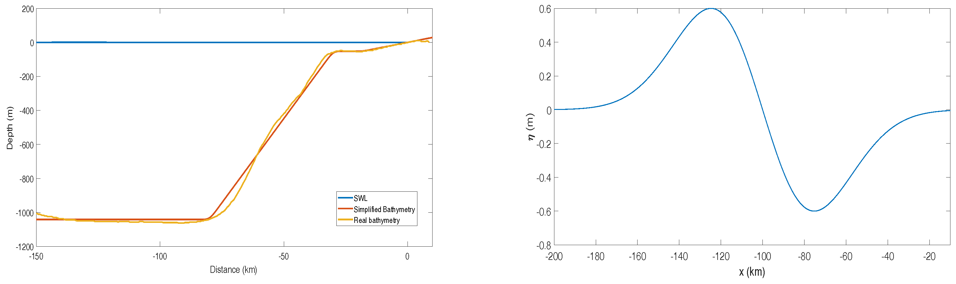
Finally, this numerical model is implemented to simulate wave run-up on simplified Aceh bathymetry. Aceh is one of the worst affected areas by the 2004 Indian Ocean tsunami. We use the same bathymetry data as mentioned in [29] which located on the west coast of Aceh. Its location is about 100 km from the epicenter of the earthquake. We simplify the bathymetry using linear piecewise function as follows.
Based on the report in [30], we use the leading depression N-waves with the wave amplitude of 0.6 m as initial waves, defined as follows.
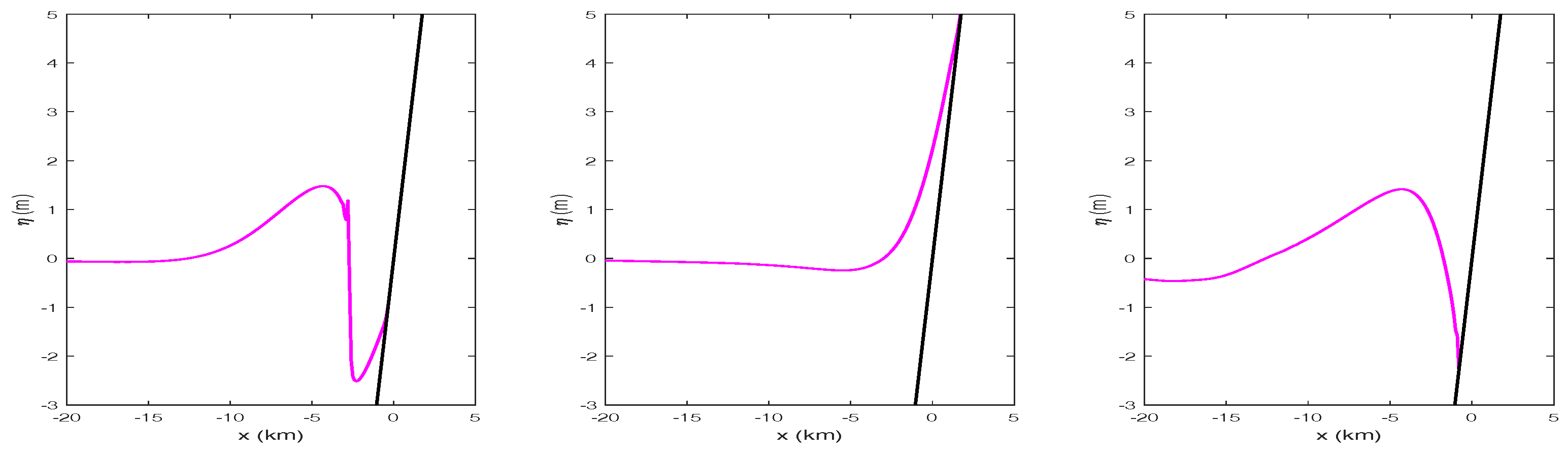
Figure 12 shows the bathymetry and the initial waves. The simplified bathymetry is close enough with the real one. The simulation is conducted for and the dynamics of moving shoreline are shown in Figure 13. Based on the simulation, the waves will arrive at the coastal area about 46 minutes. According to the tsunami travel time map by NOAA [31], the arrival time of the first wave on the west coast of Aceh is about up to one hour which is consistent with our numerical result. From the simulation, the maximum run-up is 8.02 m. Using Equation (50), the inundation area is about 2.8 km.
6. Conclusions
A two-layer non-hydrostatic model was proposed in this paper. Our numerical dispersion relation confirms the exact linear dispersion relation. A staggered finite volume method was used to approximate the governing equations in the horizontal direction, and a Keller box method resolved the vertical velocity distribution with the non-hydrostatic pressure. The predictor–corrector technique that consists of a hydrostatic and a non-hydrostatic step works well for solving the non-hydrostatic model. Having a tridiagonal matrix structure for pressure make this computation more efficient than the standard two-layer system with the pentadiagonal matrix. The numerical solution provided accurate results for non-linear and dispersive waves in a series of test cases. The numerical model is able to describe wave run-up over a sloping beach. Moreover, It gives very good agreement with the experimental data for non-linear wave transformation and evolution over a sloping beach and fringing reef. The present model accounts for wave run-up over a real bathymetry.
Author Contributions
I.M. derived the mathematical model and solved the model numerically. I.M performed the methodology, numerical investigation, writing original draft preparation, review and editing. N.E. was engaged in investigation, validation, formal analysis, review and editing. All authors have read and agreed to the published version of the manuscript.
Funding
This research was supported by the Royal Academy of Engineering and P3MI research grant.
Conflicts of Interest
The authors declare no conflict of interest.
References
- Hunt, I.A. Design of seawalls and breakwaters. J. Waterw. Harbours Div. 1959, 85, 123–152. [Google Scholar]
- Hughes, S.A. Estimation of wave run-up on smooth, impermeable slopes using the wave momentum flux parameter. Coast. Eng. 2004, 51, 1085–1104. [Google Scholar] [CrossRef]
- Hsu, T.W.; Liang, S.J.; Young, B.D.; Ou, S.H. Nonlinear run-ups of regular waves on sloping structures. Nat. Hazards Earth Syst. Sci. 2012, 12, 3811–3820. [Google Scholar] [CrossRef] [Green Version]
- Tadepalli, S.; Synolakis, C.E. The Run-Up of N-Waves on Sloping Beaches. Proc. R. Soc. Lond. Math. Phys. Eng. Sci. 1994, 445, 99–112. [Google Scholar] [CrossRef]
- Didenkulova, I. New Trends in the Analytical Theory of Long Sea Wave Runup. In Applied Wave Mathematics: Selected Topics in Solids, Fluids, and Mathematical Methods; Springer: Berlin/Heidelberg, Germany, 2009; pp. 265–296. [Google Scholar]
- Synolakis, C.E. The runup of solitary waves. J. Fluid Mech. 1987, 185, 523545. [Google Scholar] [CrossRef]
- Andadari, G.; Magdalena, I. Analytical and numerical studies of resonant wave run-up on a plane structure. J. Phys. Conf. Ser. 2019, 1321, 022079. [Google Scholar] [CrossRef]
- Erwina, N.; Pudjaprasetya, S.; Soeharyadi, Y. The Momentum conservative scheme for wave run-up on a sloping beach. Adv. Appl. Fluid Mech. 2018, 21, 493–510. [Google Scholar] [CrossRef]
- Madsen, P.A.; Murray, R.; Sørensen, O.R. A new form of the Boussinesq equations with improved linear dispersion characteristics. Coast. Eng. 1991, 15, 371–388. [Google Scholar] [CrossRef]
- Nwogu, O. Alternative Form of Boussinesq Equations for Nearshore Wave Propagation. J. Waterw. Port Coast. Ocean. Eng. 1993, 119, 618–638. [Google Scholar] [CrossRef] [Green Version]
- Wei, G.; Kirby, J.; Grilli, S.; Subramanya, R. A fully nonlinear Boussinesq model for surface waves. Part 1. Highly nonlinear unsteady waves. J. Fluid Mech. 1995, 294, 71–92. [Google Scholar] [CrossRef]
- Chorin, A.J. Numerical Solution of the Navier-Stokes Equations. Math. Comput. 1968, 22, 745–762. [Google Scholar] [CrossRef]
- Marshall, J.; Hill, C.; Perelman, L.; Adcroft, A. Hydrostatic, quasi-hydrostatic, and nonhydrostatic ocean modeling. J. Geophys. Res. Ocean. 1997, 102, 5733–5752. [Google Scholar] [CrossRef]
- Casulli, V.; Stelling, G.S. Numerical Simulation of 3D Quasi-Hydrostatic, Free-Surface Flows. J. Hydraul. Eng. 1998, 124, 678–686. [Google Scholar] [CrossRef]
- Stelling, G.; Zijlema, M. An accurate and efficient finite-difference algorithm for non-hydrostatic free-surface flow woth application to wave propagation. Int. J. Numer. Methods Fluids 2003, 43, 1–23. [Google Scholar] [CrossRef]
- Magdalena, I. Non-Hydrostatic Model for Solitary Waves Passing Through a Porous Structure. J. Disaster Res. 2016, 11, 957–963. [Google Scholar] [CrossRef]
- Arakawa, A.; Lamb, V. A potential enstrophy and energy conserving scheme for the shallow water equations. Mon. Weather Rev. 1981, 109, 18–36. [Google Scholar] [CrossRef] [Green Version]
- Stelling, G.; Duinmeijer, S. A staggered conservative scheme for every Froude number in rapidly varied shallow water flows. Int. J. Numer. Methods Fluids 2003, 43, 1329–1354. [Google Scholar] [CrossRef]
- Pudjaprasetya, S.; Magdalena, I. Momentum Conservative Scheme for Dam break and Wave Run up Simulations. East Asia J. Appl. Math. 2014, 4, 152–165. [Google Scholar] [CrossRef]
- Ma, G.; Shi, F.; Kirby, J.T. Shock-capturing non-hydrostatic model for fully dispersive surface wave processes. Ocean Model. 2012, 43–44, 22–35. [Google Scholar] [CrossRef]
- Casulli, V.; Zanolli, P. Semi-implicit numerical modeling of nonhydrostatic free-surface flows for environmental problems. Math. Comput. Model. 2002, 36, 1131–1149. [Google Scholar] [CrossRef]
- Casulli, V. A semi-implicit finite difference method for non-hydrostatic free surface flows. Int. J. Numer. Methods Fluids 1999, 30, 425–440. [Google Scholar] [CrossRef]
- Wesseling, P. Principles of Computational Fluid Dynamics; Springer: Berlin, Germany, 2000. [Google Scholar]
- Zijlema, M.; Stelling, G.; Smit, P. SWASH: An operational public domain code for simulating wave fields and rapidly varied flows in coastal waters. Coast. Eng. 2011, 58, 992–1012. [Google Scholar] [CrossRef]
- Bai, Y.; Cheung, K. Depth-intergrated free surface flow with a two-layer on-hydrostatic formulation. Int. J. Numer. Meth. Fluids 2011, 69, 411–429. [Google Scholar] [CrossRef]
- Zijlema, M.; Stelling, G. Efficient computation of surf zone waves using the nonlinear shallow water equations with non-hydrostatic pressure. Coast. Eng. 2008, 55, 780–790. [Google Scholar] [CrossRef]
- LeVeque, R.J. Finite Volume Methods for Hyperbolic Problems; Cambridge Texts in Applied Mathematics, Cambridge University Press: London, UK, 2002. [Google Scholar] [CrossRef]
- Roeber, V. Boussinesq-Type Model for Nearshore Wave Processes in Fringing Reef Environment. Ph.D. Thesis, University of Hawaii, Honolulu, HI, USA, 2010. [Google Scholar]
- Kristina, W.; Bokhove, O.; van Groesen, E. Effective coastal boundary conditions for tsunami wave run-up over sloping bathymetry. Nonlinear Process. Geophys. 2014, 21, 987–1005. [Google Scholar] [CrossRef] [Green Version]
- Leslie, J. NOAA Scientists Able to Measure Tsunami Height from Space. Available online: https://reliefweb.int/report/india/noaa-scientists-able-measure-tsunami-height-space (accessed on 28 November 2019).
- NOAA. Tsunami Travel Time Map. Available online: https://www.ngdc.noaa.gov/hazard/img/pmelwavetraveltime.gif (accessed on 28 November 2019).
Figure 1.
Sketch of two layer approach.

Figure 2.
Comparison of from exact with numerical dispersion relation.

Figure 3.
Illustration of the staggered grid with configuration of the calculated variables and .

Figure 4.
Arrangement of the unknowns in a staggered grid.

Figure 5.
Comparison of numerical solitary waves (solid line) with the analytical result (dashed-line) and SWASH result (dots) at subsequent time .
Figure 5.
Comparison of numerical solitary waves (solid line) with the analytical result (dashed-line) and SWASH result (dots) at subsequent time .

Figure 6.
Wave surface profile for at (a) , (b) , (c) , (d) . Experimental data (.), hydrostatic model (- -), and non-hydrostatic model (-).
Figure 6.
Wave surface profile for at (a) , (b) , (c) , (d) . Experimental data (.), hydrostatic model (- -), and non-hydrostatic model (-).
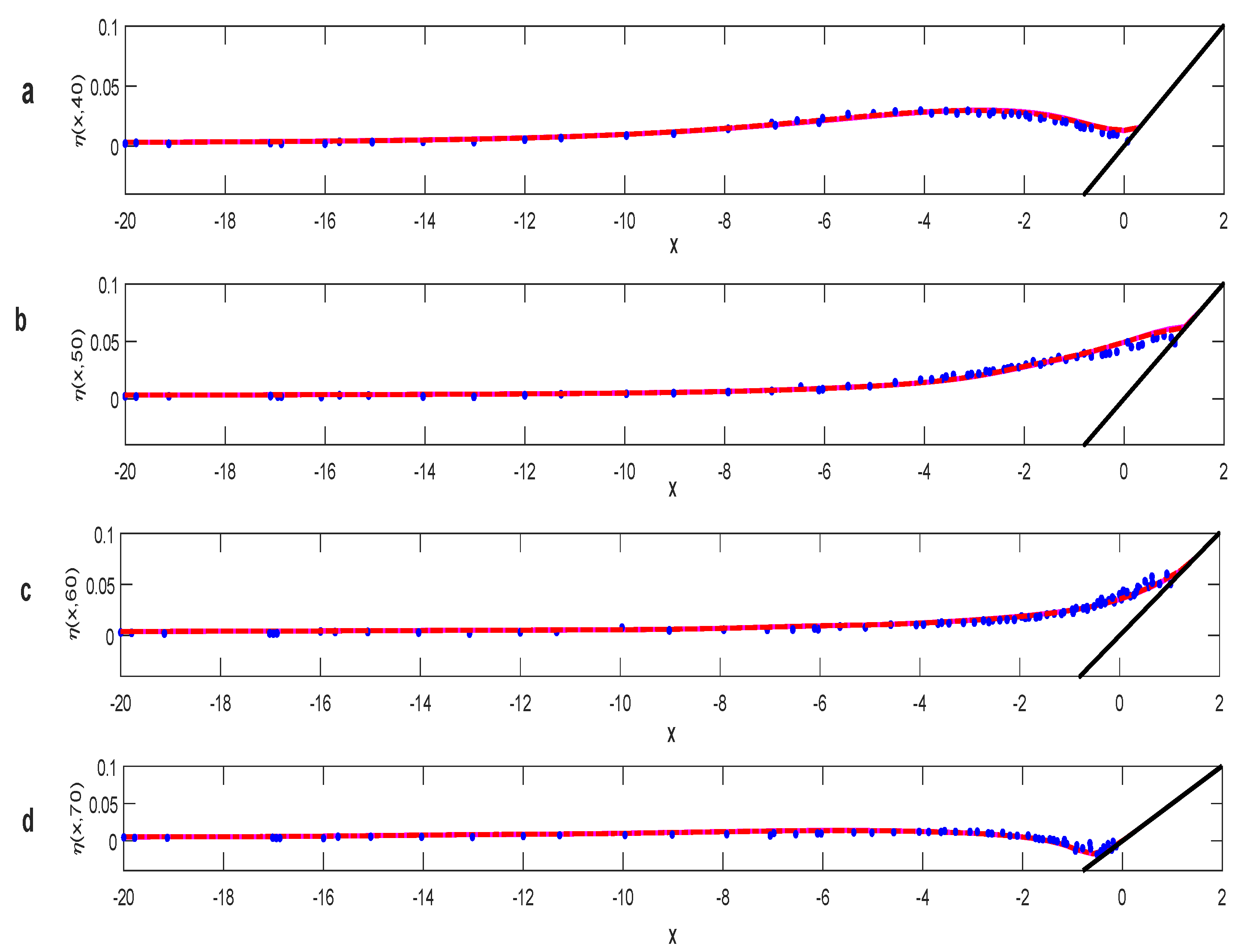
Figure 7.
Wave surface profile for at (a) , (b) , (c) , (d) . Experiment data (.), hydrostatic model (- -), and non-hydrostatic model (-).
Figure 7.
Wave surface profile for at (a) , (b) , (c) , (d) . Experiment data (.), hydrostatic model (- -), and non-hydrostatic model (-).

Figure 8.
Wave surface profile for at .
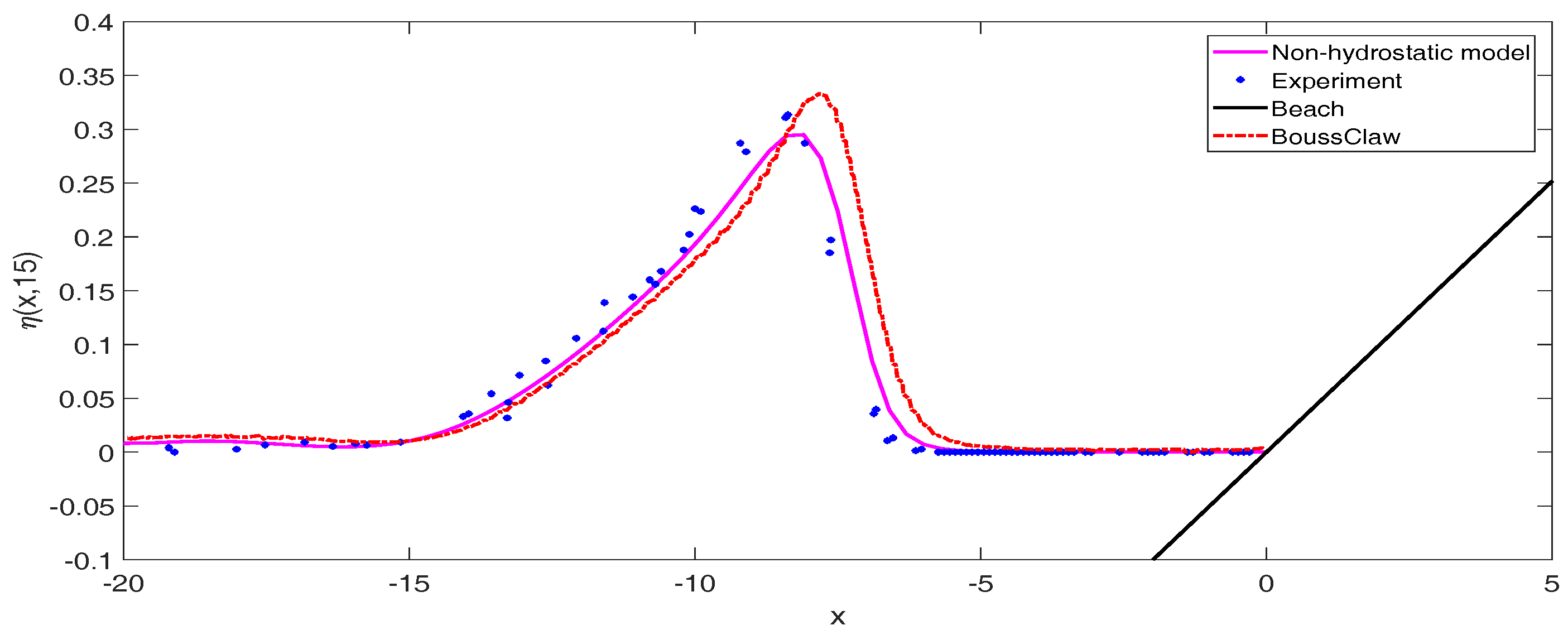
Figure 9.
Run-up solitary wave with various wave height.

Figure 10.
Transformation and surge motion of solitary wave over a fringing reef with and 1/5 slope. Numerical solution (solid line), laboratory data (circles).
Figure 10.
Transformation and surge motion of solitary wave over a fringing reef with and 1/5 slope. Numerical solution (solid line), laboratory data (circles).
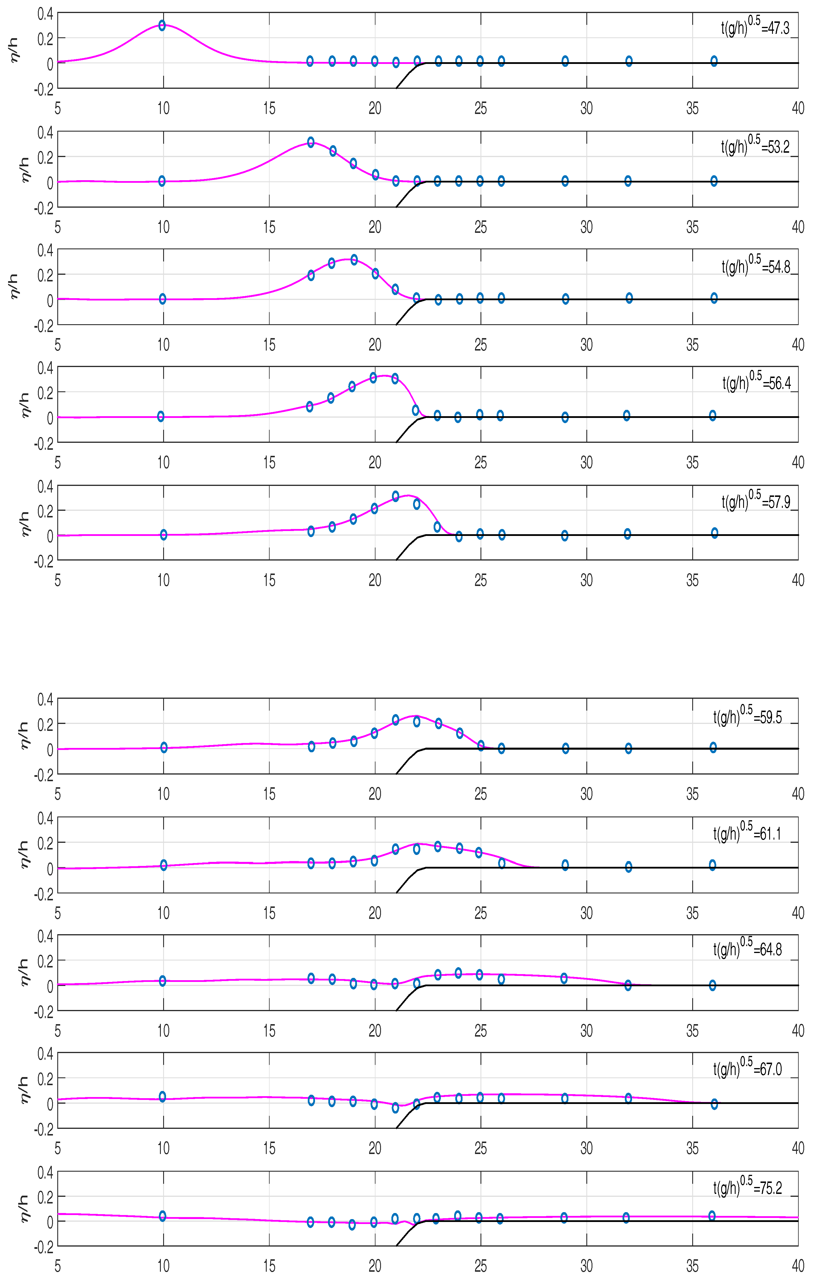
Figure 11.
A solitary wave transformation over a submerged reef crest with height 0.2, and 1/12 slope. Solid line: numerical results, circles: experimental data.
Figure 11.
A solitary wave transformation over a submerged reef crest with height 0.2, and 1/12 slope. Solid line: numerical results, circles: experimental data.
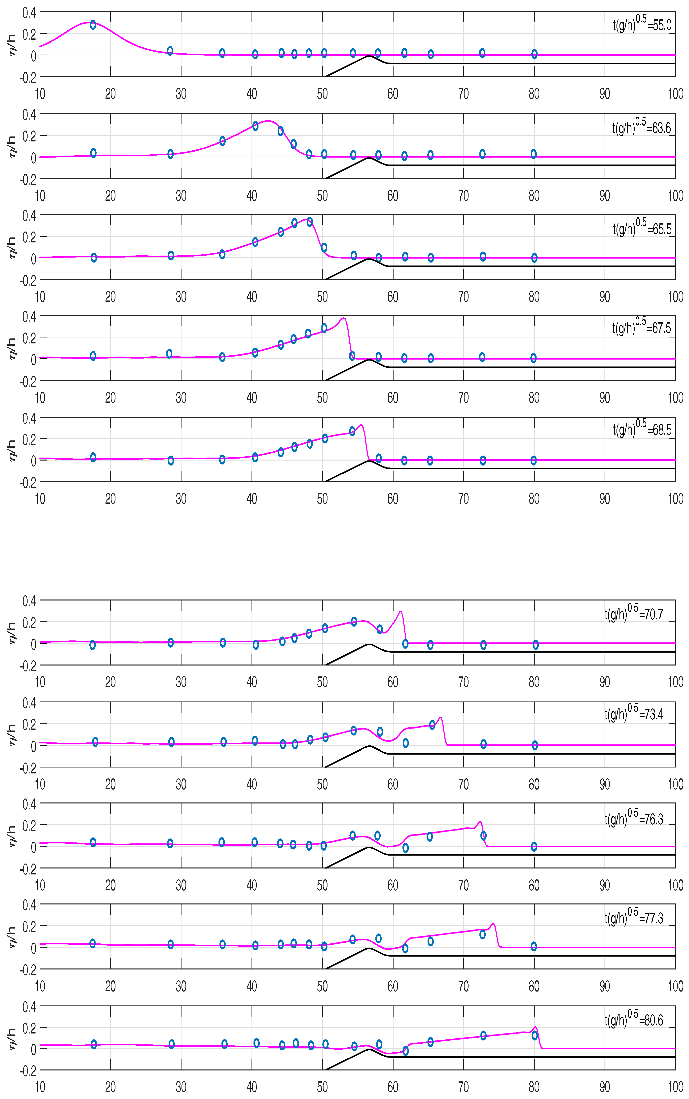
Figure 12.
Cross-section of the bathymetry of Aceh (left) and initial wave (right).

Figure 13.
Wave run-up on simplified Aceh beach at (left), (middle) and (right).

Table 1.
Error for breaking solitary wave ().
| Time | RMSE | |
|---|---|---|
| Hydrostatic Model | Non-Hydrostatic Model | |
| 15 s | 5.11% | 2.63% |
| 20 s | 5.19% | 3.46% |
© 2019 by the authors. Licensee MDPI, Basel, Switzerland. This article is an open access article distributed under the terms and conditions of the Creative Commons Attribution (CC BY) license (http://creativecommons.org/licenses/by/4.0/).
Share and Cite
MDPI and ACS Style
Magdalena, I.; Erwina, N. An Efficient Two-Layer Non-Hydrostatic Model for Investigating Wave Run-Up Phenomena. Computation 2020, 8, 1. https://0-doi-org.brum.beds.ac.uk/10.3390/computation8010001
AMA Style
Magdalena I, Erwina N. An Efficient Two-Layer Non-Hydrostatic Model for Investigating Wave Run-Up Phenomena. Computation. 2020; 8(1):1. https://0-doi-org.brum.beds.ac.uk/10.3390/computation8010001
Chicago/Turabian StyleMagdalena, Ikha, and Novry Erwina. 2020. "An Efficient Two-Layer Non-Hydrostatic Model for Investigating Wave Run-Up Phenomena" Computation 8, no. 1: 1. https://0-doi-org.brum.beds.ac.uk/10.3390/computation8010001
Note that from the first issue of 2016, this journal uses article numbers instead of page numbers. See further details here.