Nondimensional Characterization of the Operational Envelope of a Wet Friction Clutch


 and
and
Abstract
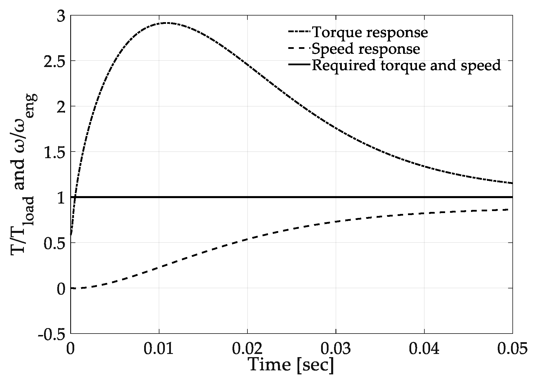
:1. Introduction
2. Fluid Film Model
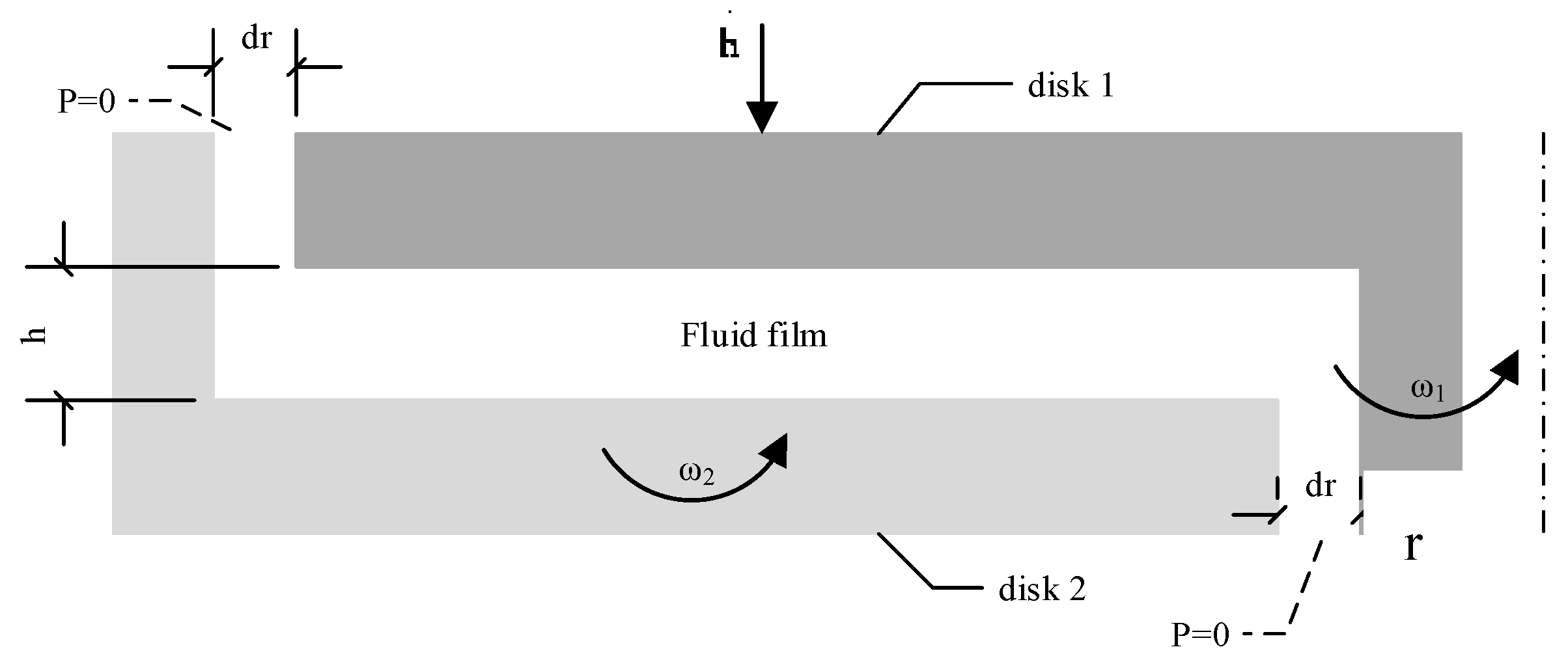
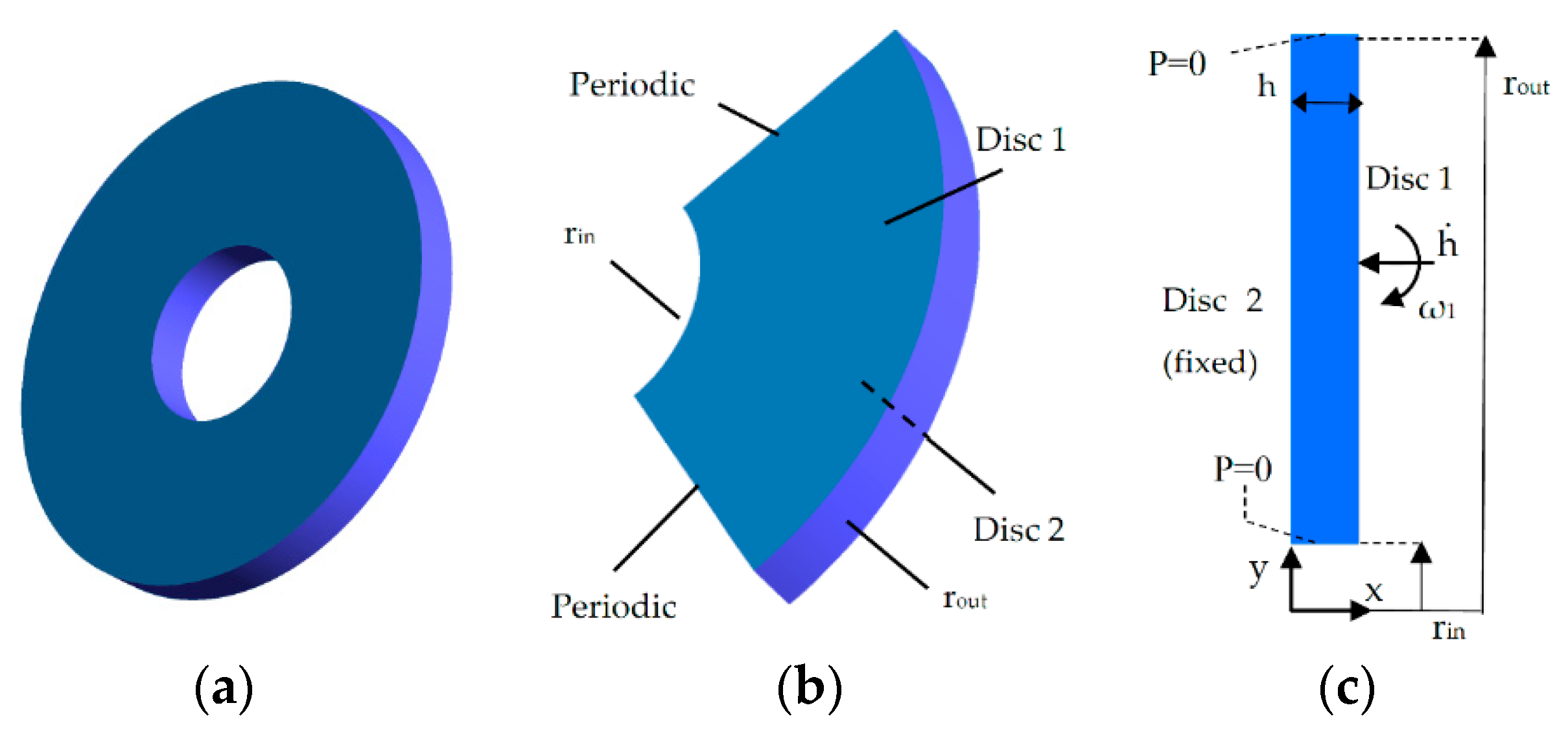
2.1. Geometry Modifications and Basic Parameters
2.2. Flow Equations
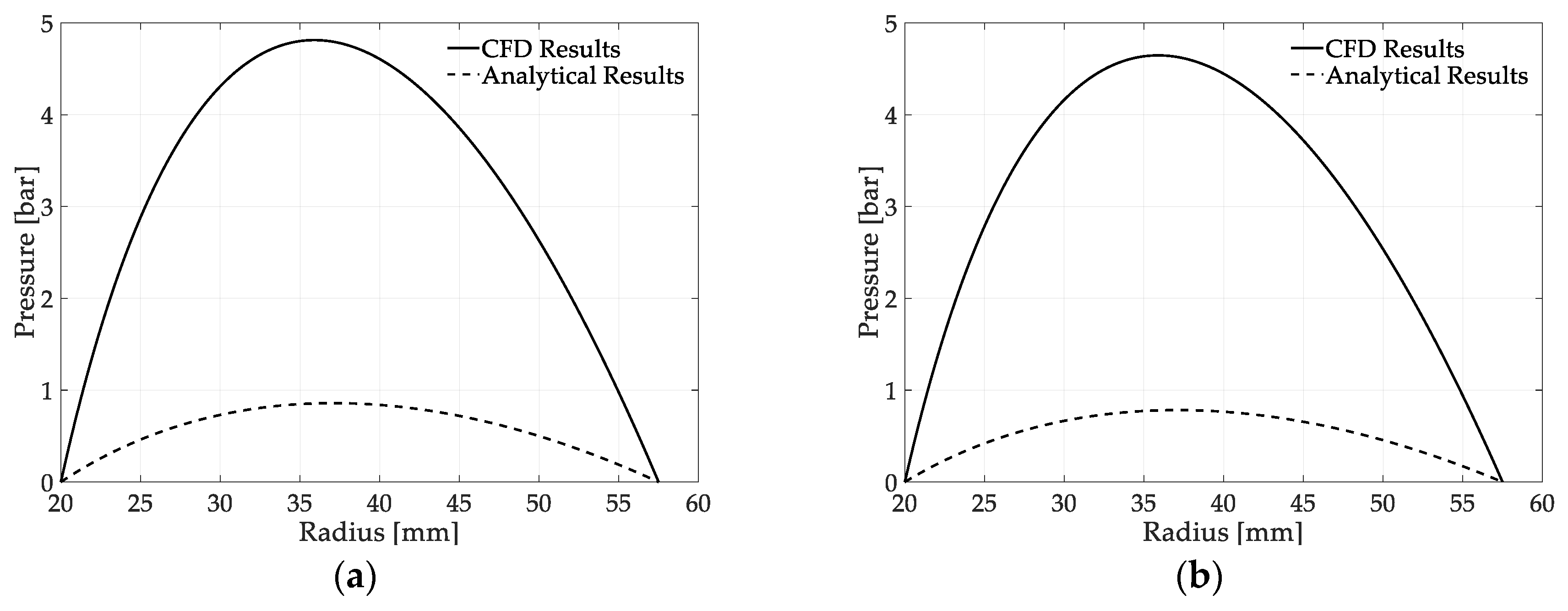
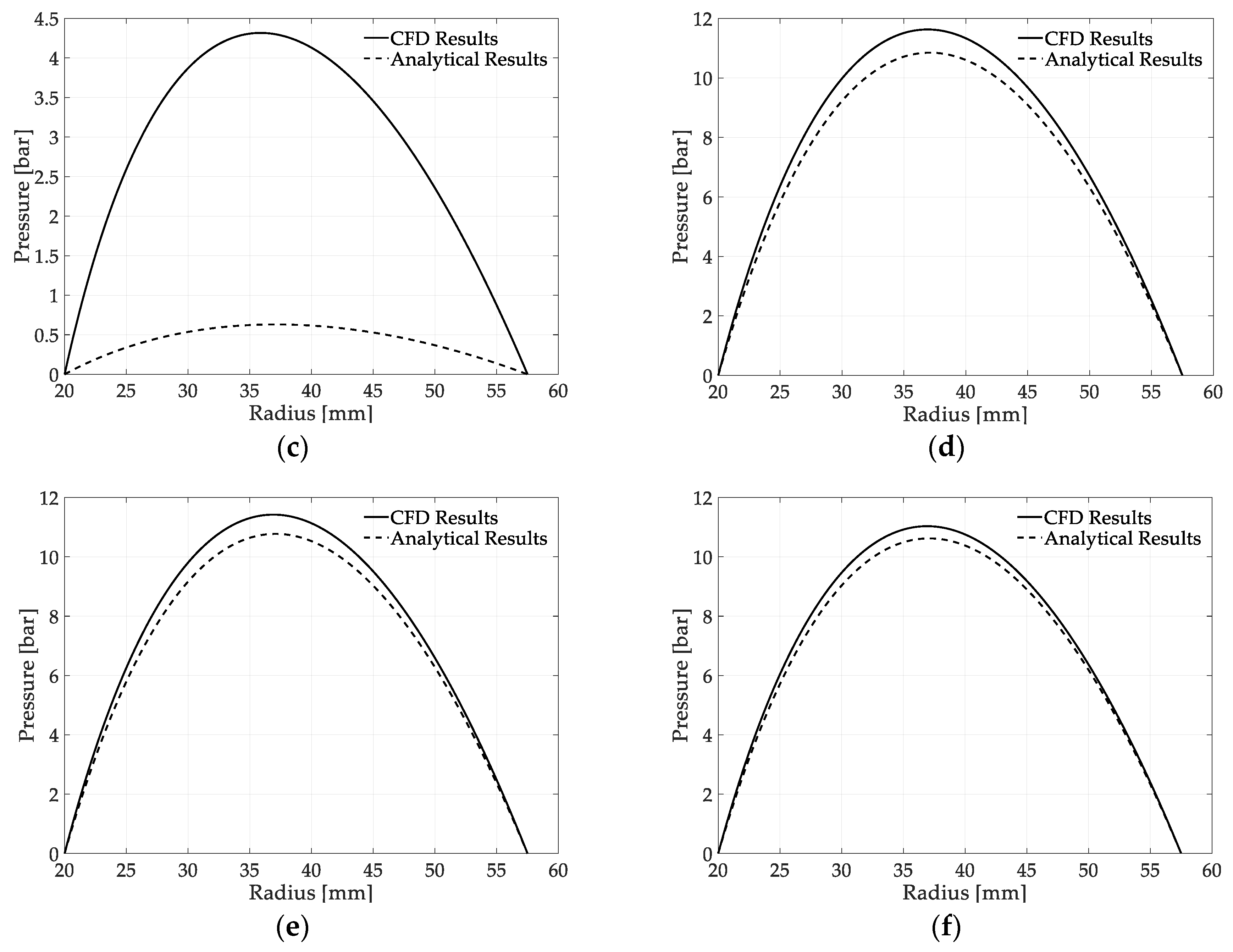
3. Analytical Solutions and CFD Results
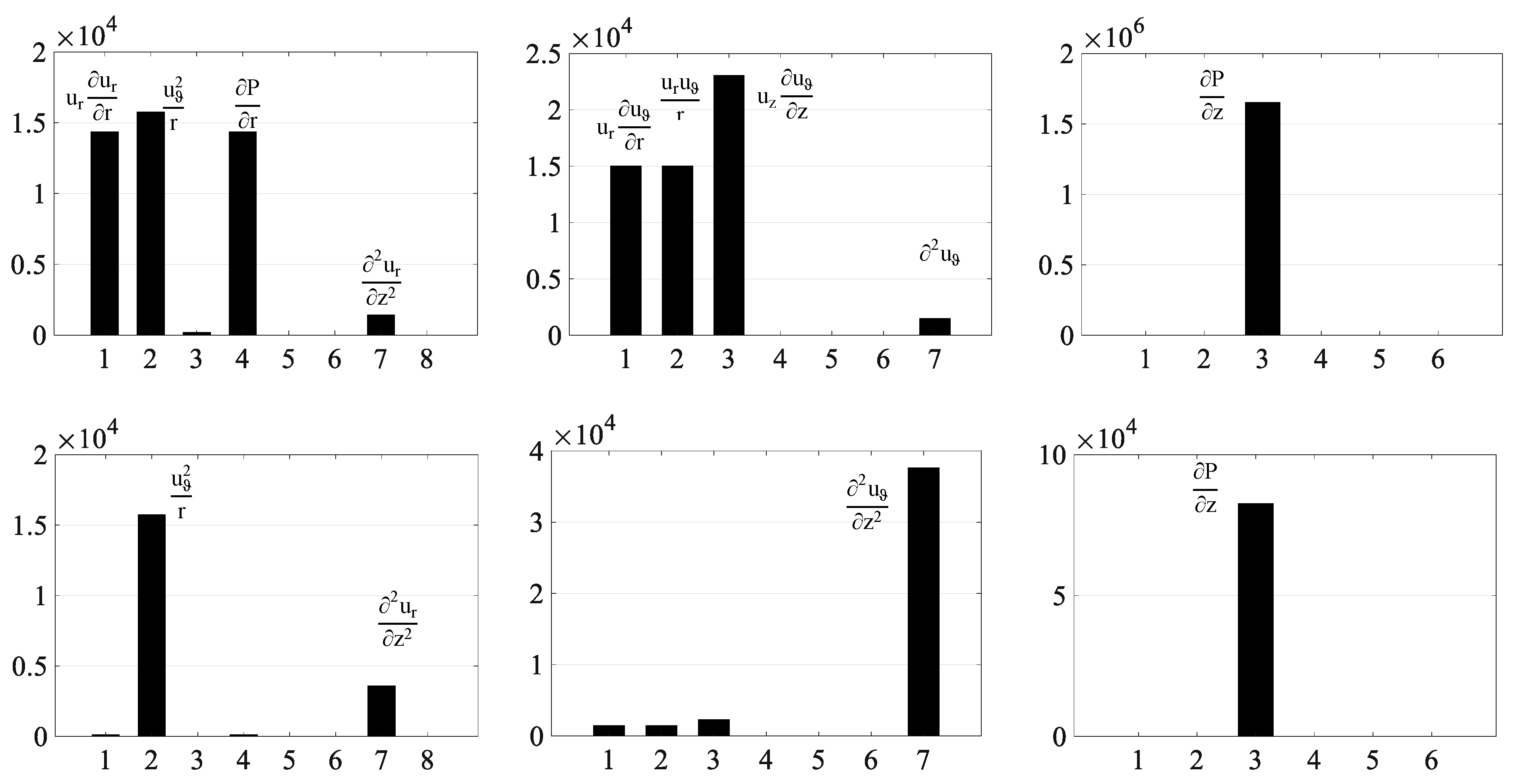
3.1. Analytical Solutions
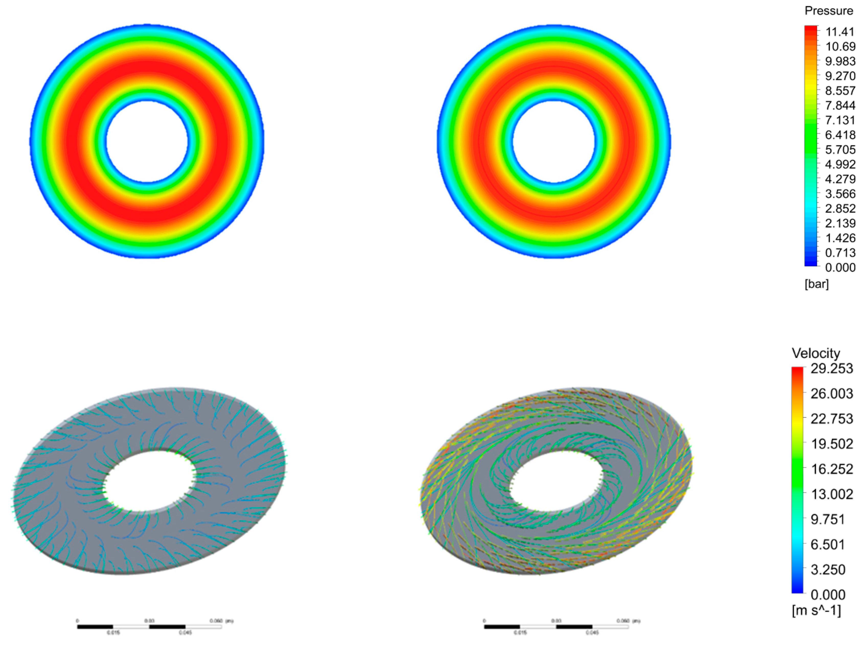
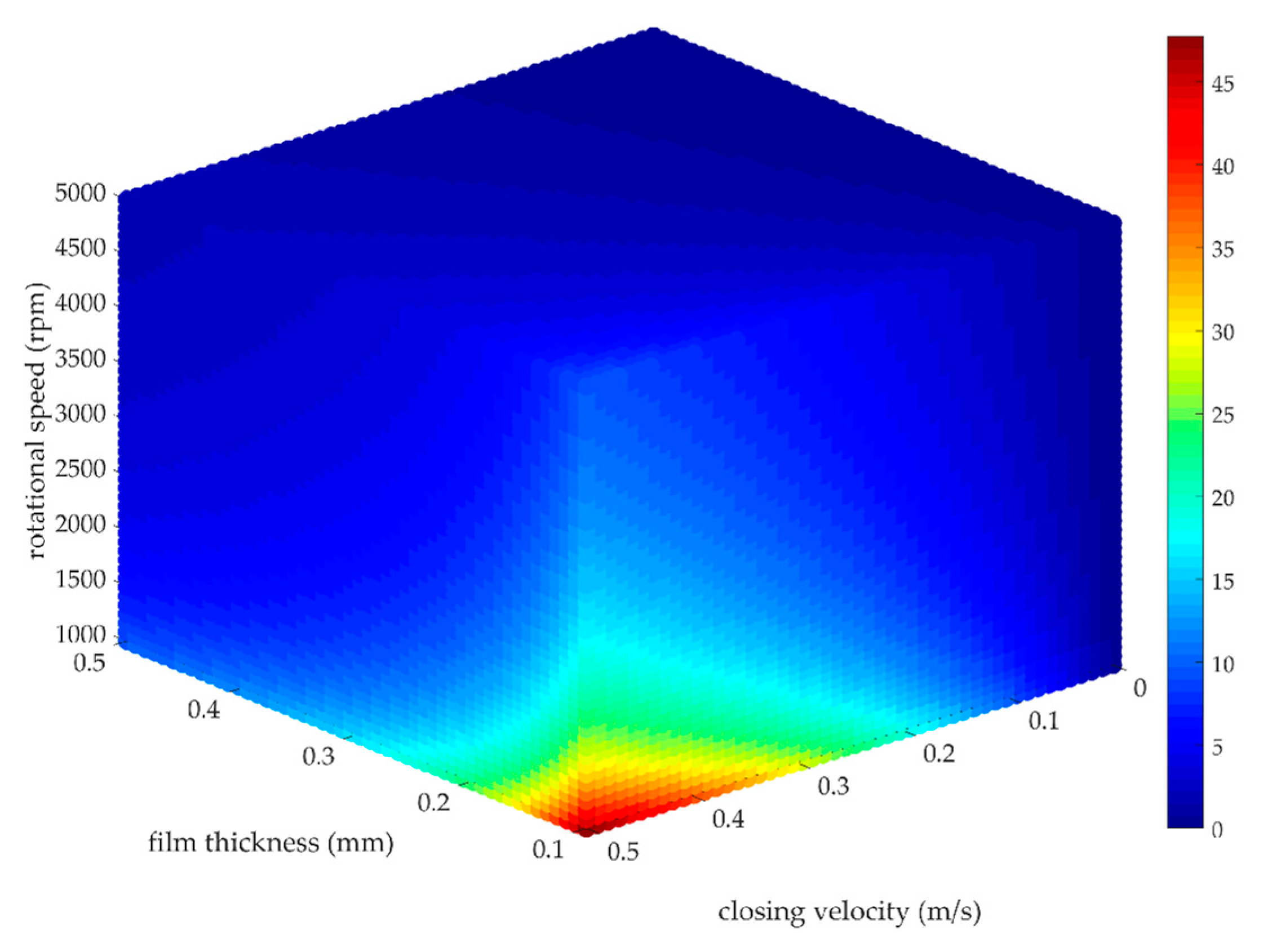
3.2. Computational Model
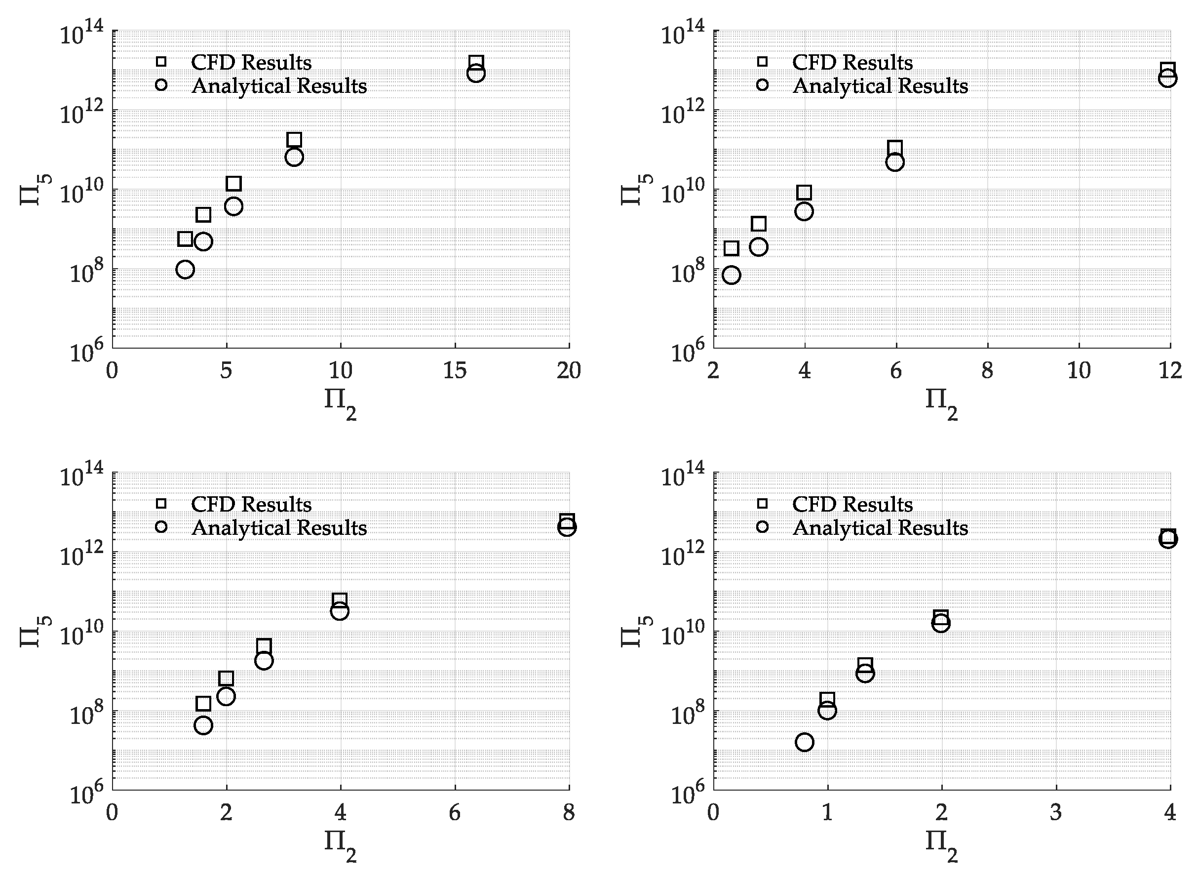
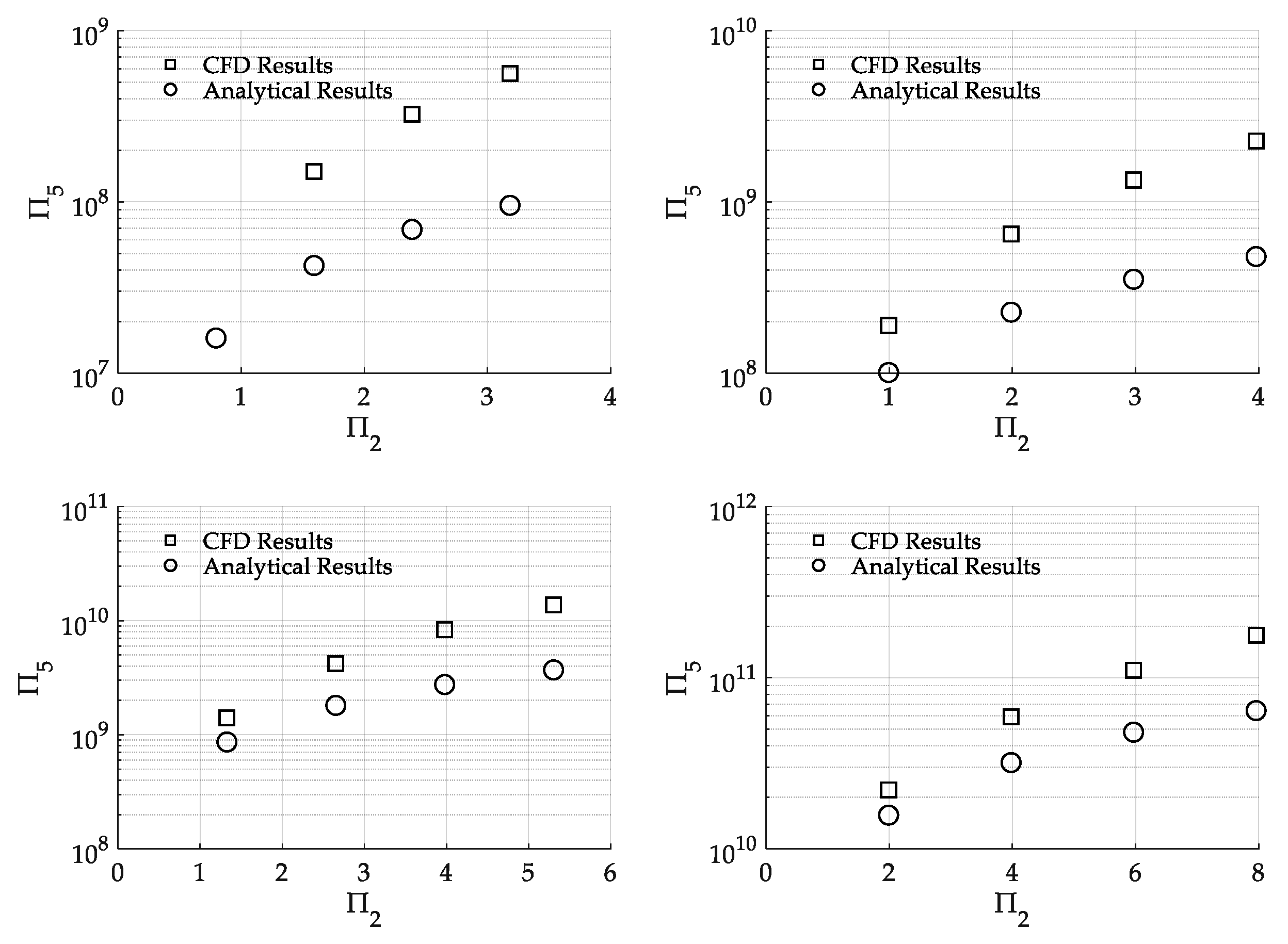
4. Nondimensional Analysis and Post-Process of CFD Results
4.1. Creation of Nondimensional Numbers
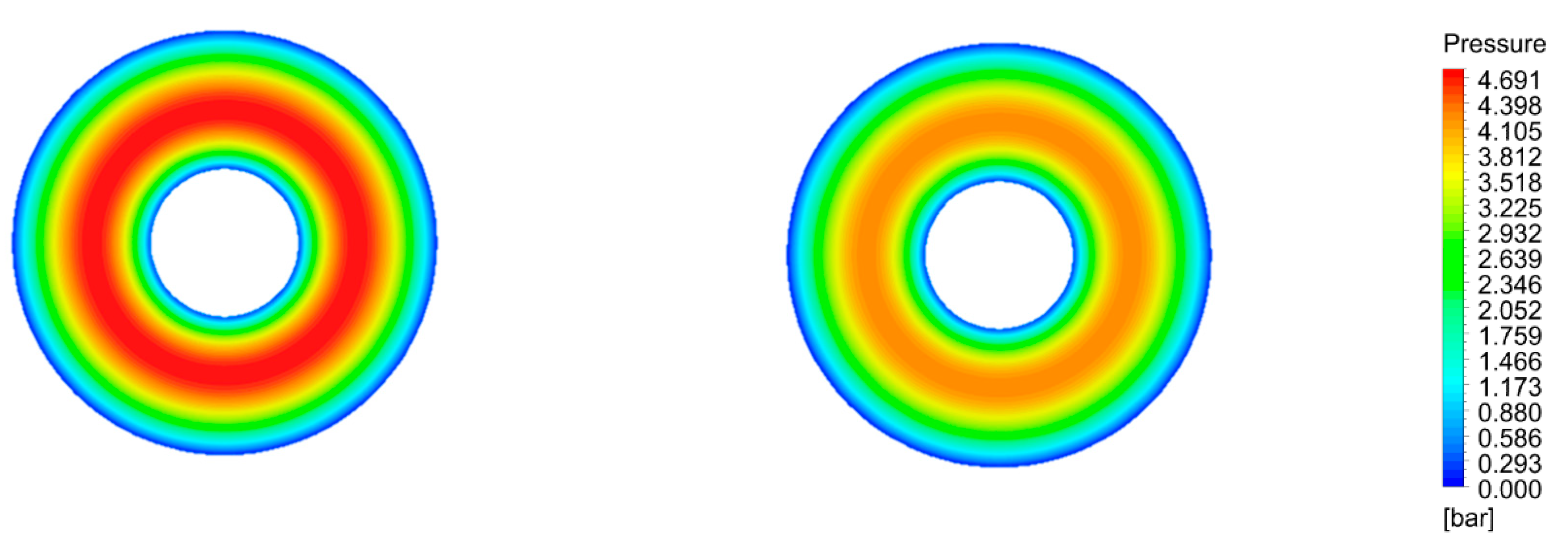
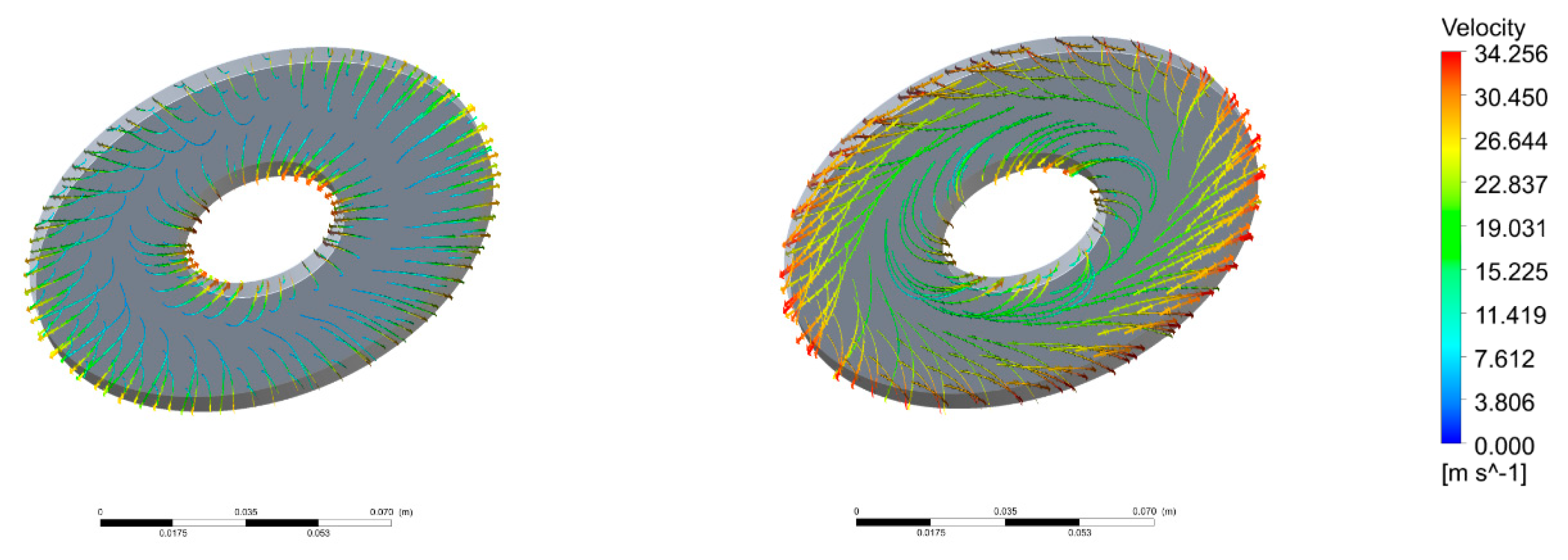
4.2. Post-Processing of CFD Results
5. Conclusions
Author Contributions
Funding
Acknowledgments
Conflicts of Interest
References
- Wang, Y.; Li, Y.; Liu, Y.; Zhang, W. Modeling and experimental research on engaging characteristics of wet clutch. Ind. Lubr. Tribol. 2019, 71, 94–101. [Google Scholar] [CrossRef]
- Cho, J.; Lee, Y.; Kim, W.; Jang, S. Wet single clutch engagement behaviors in the dual-clutch transmission system. Int. J. Automot. Technol. 2018, 19, 463–472. [Google Scholar] [CrossRef]
- Iqbal, S.; Al-Bender, F.; Pluymers, B.; Desmet, W. Mathematical model and experimental evaluation of drag torque in disengaged wet clutches. Isrn Tribol. 2013, 2013, 206539. [Google Scholar] [CrossRef] [Green Version]
- Aphale, C.R.; Cho, J.; Schultz, W.W.; Ceccio, S.L.; Yoshioka, T.; Hiraki, H. Modeling and parametric study of torque in open clutch plates. J. Tribol. 2006, 128, 422–430. [Google Scholar] [CrossRef] [Green Version]
- Yuan, Y.; Liu, E.A.; Hill, J.; Zou, Q. An improved hydrodynamic model for open wet transmission clutches. J. Fluids Eng. 2007, 129, 333–337. [Google Scholar] [CrossRef]
- Fujii, Y.; Kapas, N.; Tseng, J. Clutch Wet. In Encyclopedia of Automotive Engineering; John Wiley & Sons: New York, NY, USA, 2014; pp. 1–15. [Google Scholar] [CrossRef]
- Neupert, T.; Benke, E.; Bartel, D. Parameter study on the influence of a radial groove design on the drag torque of wet clutch discs in comparison with analytical models. Tribol. Int. 2018, 119, 809–821. [Google Scholar] [CrossRef]
- Zhang, L.; Wei, C.; Hu, J.B. Model for the prediction of drag torque characteristics in wet clutch with radial grooves. Proc. Inst. Mech. Eng. Part D: J. Automob. Eng. 2019, 233, 3043–3056. [Google Scholar] [CrossRef]
- Wu, P.H.; Zhou, X.; Yang, C.; Lv, H.; Lin, T.; Wu, X. Parametric analysis of the drag torque model of wet multi-plate friction clutch with groove consideration. Ind. Lubr. Tribol. 2018, 70, 1268–1281. [Google Scholar] [CrossRef]
- Wu, P.; Xu, J.; Zhou, X.-J. Numerical and experimental research on engagement process of wet multi-plate friction clutches with groove consideration. Proc. Inst. Mech. Eng. Part J J. Eng. Tribol. 2019, 233, 1464–1482. [Google Scholar] [CrossRef]
- Pardeshi, I.; Shih, T.I. A Computational Fluid Dynamics Methodology for Predicting Aeration in Wet Friction Clutches. ASME. J. Fluids Eng. 2019, 141, 121304. [Google Scholar] [CrossRef]
- Wu, W.; Xiong, Z.; Hu, J.; Yuan, S. Application of CFD to model oil–air flow in a grooved two-disc system. Int. J. Heat Mass Transf. 2015, 91, 293–301. [Google Scholar] [CrossRef]
- Neupert, T.; Bartel, D. High-resolution 3D CFD multiphase simulation of the flow and the drag torque of wet clutch discs considering free surfaces. Tribol. Int. 2019, 129, 283–296. [Google Scholar] [CrossRef]
- Aphale, C.R.; Schultz, W.W.; Ceccio, S.L. Aeration in lubrication with application to drag torque reduction. J. Tribol. 2011, 133, 031701. [Google Scholar] [CrossRef]
- Launder, B.; Poncet, S.; Serre, E. Laminar, transitional, and turbulent flows in rotor stator cavities. Ann. Rev. Fluid Mech. 2010, 42, 229–248. [Google Scholar] [CrossRef] [Green Version]
- Huang, J.; Wei, J.; Qiu, M. Laminar flow in the gap between two rotating parallel frictional plates in hydro-viscous drive. Chin. J. Mech. Eng. 2012, 25, 144–152. [Google Scholar] [CrossRef]
- Bassi, A.; Milani, M.; Montorsi, L.; Terzi, S. Dynamic analysis of the lubrication in a wet clutch of a hydromechanical variable transmission. SAE Int. J. Commer. Veh. 2016, 9, 280–290. [Google Scholar] [CrossRef] [Green Version]
- Daily, J.W.; Nece, R.E. Chamber dimension effects on induced flow and frictional resistance of enclosed rotating disks. ASME J. Basic Eng. 1960, 82, 217–232. [Google Scholar] [CrossRef]
- Haddadi, S.; Poncet, S. Turbulence modeling of torsional Couette flows. Int. J. Rotating Mach. 2008, 2008, 635138. [Google Scholar] [CrossRef] [Green Version]
- Spurk, H.J.; Askel, N. Fluid Mechanics, 3rd ed.; Springer Nature Switzerland AG: Basel, Switzerland, 2020. [Google Scholar]
- ANSYS Fluent Theory Guide; ANSYS, Inc.: Canonsburg, PA, USA, 2013.
- Gibbings, J.C. Dimensional Analysis; Springer: London, UK, 2011; pp. 55–82. [Google Scholar]


| Symbol | Description | Value | Unit |
|---|---|---|---|
| rout | Outer radius | 57.5 | mm |
| rin | Inner radius | 20 | mm |
| h | Film thickness | 0.1–0.5 | mm |
| Gap closing velocity | 0–0.5 | m/s | |
| ω1 | Disc 1 rot. speed. | 1000–5000 | rpm |
| ω2 | Disc 2 rot speed. | 0 | rpm |
| μ | Dynamic viscosity | 0.01 | Pa s |
| ρ | Density | 800 | kg/m3 |
| h [mm] | ω1 [rpm] | |
|---|---|---|
| 0.5 | 0.5 | 1000 |
| 0.4 | 0.375 | 2000 |
| 0.3 | 0.25 | 3000 |
| 0.2 | 0.125 | 4000 |
| 0.1 | 0 | 5000 |
© 2020 by the authors. Licensee MDPI, Basel, Switzerland. This article is an open access article distributed under the terms and conditions of the Creative Commons Attribution (CC BY) license (http://creativecommons.org/licenses/by/4.0/).
Share and Cite
Rogkas, N.; Vakouftsis, C.; Vasileiou, G.; Manopoulos, C.; Spitas, V. Nondimensional Characterization of the Operational Envelope of a Wet Friction Clutch. Computation 2020, 8, 21. https://0-doi-org.brum.beds.ac.uk/10.3390/computation8010021
Rogkas N, Vakouftsis C, Vasileiou G, Manopoulos C, Spitas V. Nondimensional Characterization of the Operational Envelope of a Wet Friction Clutch. Computation. 2020; 8(1):21. https://0-doi-org.brum.beds.ac.uk/10.3390/computation8010021
Chicago/Turabian StyleRogkas, Nikolaos, Christos Vakouftsis, Georgios Vasileiou, Christos Manopoulos, and Vasilios Spitas. 2020. "Nondimensional Characterization of the Operational Envelope of a Wet Friction Clutch" Computation 8, no. 1: 21. https://0-doi-org.brum.beds.ac.uk/10.3390/computation8010021