Brain Tissue Evaluation Based on Skeleton Shape and Similarity Analysis between Hemispheres
by
 , , and
Lenuta Pana
1,2, 
Simona Moldovanu
2,3 ,
,
Nilanjan Dey
4 ,
,
Amira S. Ashour
5 and
Luminita Moraru
1,2,* 1
Faculty of Sciences and Environment, Department of Chemistry, Physics& Environment, Dunarea de Jos University of Galati, 47 Domneasca Str., 800008 Galati, Romania
2
The Modelling & Simulation Laboratory, Dunarea de Jos University of Galati, Galati 47 Domneasca Str., 800008 Galati, Romania
3
Faculty of Automation, Computers, Electrical Engineering and Electronics, Department of Computer Science and Information Technology, Dunarea de Jos University of Galati, Galati 47 Domneasca Str., 800008 Galati, Romania
4
Department of Information Technology, Techno India College of Technology, West Bengal 700156, India
5
Department of Electronics and Electrical Communications Engineering, Faculty of Engineering, Tanta University, Tanta 31527, Egypt
*
Author to whom correspondence should be addressed.
Computation 2020, 8(2), 31; https://0-doi-org.brum.beds.ac.uk/10.3390/computation8020031
Submission received: 7 March 2020
/
Revised: 9 April 2020
/
Accepted: 12 April 2020
/
Published: 15 April 2020
(This article belongs to the Special Issue Selected Papers from the 8th International Conference on Experiments/Process/System Modeling/Simulation/Optimization (IC-EPSMSO 2019))
Abstract
:Background: The purpose of this article is to provide a new evaluation tool based on skeleton maps to assess the tumoral and non-tumoral regions of the 2D MRI in PD-weighted (proton density) and T2w (T2-weighted type) brain images. Methods: The proposed method investigated inter-hemisphere brain tissue similarity using a mask in the right hemisphere and its mirror reflection in the left one. At the hemisphere level and for each ROI (region of interest), a morphological skeleton algorithm was used to efficiently investigate the similarity between hemispheres. Two datasets with 88 T2w and PD images belonging to healthy patients and patients diagnosed with glioma were investigated: D1 contains the original raw images affected by Rician noise and D2 consists of the same images pre-processed for noise removal. Results: The investigation was based on structural similarity assessment by using the Structural Similarity Index (SSIM) and a modified Jaccard metrics. A novel S-Jaccard (Skeleton Jaccard) metric was proposed. Cluster accuracy was estimated based on the Silhouette method (SV). The Silhouette coefficient (SC) indicates the quality of the clustering process for the SSIM and S-Jaccard. To assess the overall classification accuracy an ROC curve implementation was carried out. Conclusions: Consistent results were obtained for healthy patients and for PD images of glioma. We demonstrated that the S-Jaccard metric based on skeletal similarity is an efficient tool for an inter-hemisphere brain similarity evaluation. The accuracy of the proposed skeletonization method was smaller for the original images affected by Rician noise (AUC = 0.883 (T2w) and 0.904 (PD)) but increased for denoised images (AUC = 0.951 (T2w) and 0.969 (PD)).
1. Introduction
Over the last decades brain diseases have become increasingly frequent. Most clinical researches show that many patients diagnosed with brain tumors die due to inaccurate detection of the position and size of the tumor. MRI (Magnetic Resonance Imaging) scanning is pointed at the intracranial cavity, producing a complete image of the brain, which is then visually examined for diagnosis of cerebral affections [1,2,3,4,5]. Glioma is the most common malign tumor in the central nervous system making up approximately 80% of total malign brain tumors. Full surgical removal is almost impossible due to the tumor’s location and infiltration [6,7].
In a comparative study of real-world objects, the human eye marks the edges of objects. In the diagnosis of cerebral affections, the edges of the image are important elements of analysis. In image processing, edge detection is a complex process often requiring convolutions between first-order derivative filters [8], second order filters [9], or the image gradient [10,11] and the original image. Glioma tumors show a higher heterogeneity and irregularity of the tumor tissue. This complex structure qualifies the edge detection and skeletonization to distinguish between the tumor area and the normal tissue. To estimate edge detection with a good accuracy, as well as to assess the brain MRI image segmentation, a number of similarity indices have been defined such as feature similarity index (FSSIM), mean SSIM, and SSIM [8,12] or Jaccard [13]. A similarity study between cerebral hemispheres requests an effective and accurate method for edge detection because an inappropriate choice leads to the extraction of erroneous information/edges.
Several skeletonization algorithms have been devoted to process 2D or 3D images in various applications [14,15,16,17,18,19,20]. Lee and Kashyap [14] introduced a 3D thinning algorithm to extract medial surfaces and medial axes by preserving Euler characteristics and connectivity in the original object. The noise was removed during the pre-processing step and in the post-processing steps the skeleton was extracted, where the unwanted branches were removed, and a thinning operation was performed. The authors claimed the proposed algorithm outperformed the existing skeletonization algorithms in casting and forging manufacturing processes. In addition, other studies were devoted to evaluate and/or monitor brain tumors. Wu et al. [16] designed an adaptive superpixel generation using a hybrid algorithm based on an automated selection of the number of superpixels for further glioma segmentation in T2w MRI images. Afterward, feature extraction, (such as statistical, texture, curvature and fractal features, for each superpixel, and a support vector machine (SVM) for classification were applied. The ASLIC0 algorithm was based on simple linear iterative clustering version with 0 parameters for a hyper-parameter K selection and optimization. The results reported 0.8492 average Dice, 81.47% sensitivity, 99.64% specificity, and Hausdorff distance of 3.4697 pixels. Zhao et al. [17] developed a decision support algorithm for detection and segmentation of abnormal tissue regions and brain tumor/glioma in MRI, based on the learn structure of undirected graphical models. The superpixel, statistical feature extraction from the superpixel distribution, and the Conditional Random Fields (CRF) for image segmentation, were used. This method led to more regular superpixel shape, but with high computational cost. Yang et al. [18] obtained a smooth and accurate skeleton of a specified object in the gray image using the level set idea combined with a gradient module method. First, the object’s boundary was detected based on Partial Differential Equation PDE and level set method. Then, the skeleton of the object was determined by connecting endpoints through the shortest path algorithm. The reported method provided good results and was insensitive to noise. Shen et al. [19] provided an elaborated skeleton extraction in a natural image method based on a holistically-nested network (fully convolutional network FC-N) with multiple scale-associated side outputs for skeleton extraction. This complex algorithm provided improved recall and precision at most of the precision-recall regimes.
In this study, a method for edge detection in the brain structure based on a skeleton algorithm and morphological mathematical operations is proposed [20]. The proposed algorithm is implemented in two steps. In the first step, erosion and opening morphological operations are used. A strel object or a morphological structuring element is used for a finite number of times to perform the morphological operation. In the second step, the same strel object is called the same number of times to run morphological dilatation. The image is dilated and, at the end, the union of all intermediate steps leads to the skeleton of the image. Skeletal similarity analysis is performed on the regions of interest symmetrically placed on both hemispheres. To cut the regions of interest, a mask is designed on the brain tissue. The reference is healthy patients and the source is patients diagnosed with glioma. The skeletal similarity is calculated using SSIM and S-Jaccard between the corresponding interest regions. Moreover, SSIM and S-Jaccard values are clustered using the Silhouette method (SV) [21]. The quality of the clusters is analyzed with the Silhouette coefficient (SC). To validate our analysis and assess the overall classification accuracy, ROC curve implementation was carried out [22]. Also, a skeletal similarity empirical method using the comparison of the trend lines of skeleton map datasets to determine a possible perceived similarity or dissimilarity based on a certain pattern is proposed. The analysis was performed in two datasets; D1 contains raw images from the Harvard’s Whole Brain Atlas that are affected by noises with Rician distribution. D2 contains denoised images by using an anisotropic diffusion filter [23,24]. The results are compared in terms of the noise effect on the proposed method.
2. Materials and Methods
2.1. Mathematical Approaches
(a) SSIM quantifies image quality or perceptual difference between two images as a result of various processing operations. It is based on the computation of luminance, contrast, and structural terms. For x and y binary images, SSIM is defined as [8]:
where μx, μy,σx, σy, σxy are the local means, standard deviations, and cross-covariance for images x and y. Usually, , L being the dynamic range of pixel values (255 for 8-bit images), 𝐾1 << 1 and c2 = c1/2.
(b) The skeleton algorithm of an image A, which represents a region of interest (ROI), is performed through the following steps:
(b1) Morphological erosion and opening operations are run using a morphological structuring element B and are repeated k times. The process stops after locating the ‘last’ contour pixel in the shape [20,25]. k is the last iterative step before the object erodes into the void space (i.e., erosion takes place up to the point where, if one would repeat the process one more time, the object would be confused with the background, that is, there would be no object).
(b2) Dilation is performed with the morphological dilatation function and the structural element B. This operation is repeated k times.
For both morphological operations (erosion and dilation) the morphological structuring element B is a disc with a radius of 5.
(c) The Jaccard index represents the ratio between the intersection and union of two binary images. HL represents the cardinal of ROI cuts from the left hemisphere and HR the cardinal of ROI cuts from the right hemisphere, respectively [13].
We refer the Jaccard index as the S-Jaccard as its application follows the skeleton operation.
(d) k-means algorithm for clustering allows division of a dataset into a specific number of groups. High quality clusters with high intra-cluster similarity and low inter-cluster similarity represent a good clustering operation [1]. First, k-means calculates k centroids and then it attributes each observation to the nearest cluster. These two steps are alternated until a stopping criterion is met, when there is no further change in the assignment of the data points. The k-means algorithm aims at minimizing an objective function, which in this case is the squared error function between μk and the data point in cluster ck [21,26,27]:
where is the Euclidean distance between a data point, xi, and a cluster center, μk, iterated over ith all k points in the cluster, for all k clusters. In our study, k = 3.
(e) The Silhouette method computes the silhouette width for each object, the average silhouette width of each cluster, and the overall average silhouette width for the entire image set. This index shows how proper a cluster is separated from its neighbors. By computing the silhouette index, it is possible to assess the validity of a clustering operation. Also, the correctness regarding the number of selected clusters can be evaluated [12,28]. The silhouette of the object i, S(i):
where a(i) is the average dissimilarity between observation i and other points in its own cluster (‘within’ dissimilarity), and b(i) denotes the minimum average dissimilarity of i to all observations of other clusters (between’ dissimilarity).
The Silhouette coefficient is .
For, SC ∈ [0.81–1.00], the object is very well-clustered; SC ∈ [0.51–0.80] the object is well-clustered; SC∈ [0.26–0.50] the object is poor-clustered, and SC ≤ 0.25 occurs with the artificial cluster [26]. Accordingly, when S(i) is close to 1, the ‘within’ dissimilarity a(i) is much smaller than the smallest ‘between’ dissimilarity b(i), and the object is ‘well-clustered’, while for S(i)–0, the a(i), and b(i) are approximately equal; thus, it is unclear as to which cluster the object i is assigned. Also, s(i) close to–1, refers to a misclassified object.
(f) Skeletal similarity empirical method. The trend lines are generated for each analyzed region of interest ROI and brain hemisphere by computing the length of each skeleton segment in each skeleton map. The ROIs belonging to the healthy brain hemisphere are used as reference images. The ROIs belonging to the tumoral regions are so called source images. The length of each segment in the skeleton map is determined using the Cartesian coordinates of the start and end points and the Euclidian distance. A scatter plot displaying the relationship between the length of each skeletal segment and the number of segments having the same length is built. A second-degree polynomial function provides the best fit for approximation. The similarity of the polynomial curves is an indicator of the structural similarity between the healthy/reference and the source skeleton map and allow us to estimate the new edges generated empirically due to the tumor presence.
The images provided by the Harvard’s Whole Brain Atlas are raw images and are affected by Rician noise. The selected ROIs are denoised by using an anisotropic diffusion filter [23,24]. The anisotropic diffusion filtering provides reliable noise removing while very satisfactory edge-preserving results are achieved. The noise removal results are quantitatively assessed by the signal-to-noise ratio (SNR).
2.2. Subjects, Image Acquisition and Post-Processing
The programming environment was a MATLAB R2017a and Image Processing toolbox. The hardware was a computer with the following technical performance: Inter (R) Core (TM) i7-8550U CPU @ 1.80 GHz; Memory (RAM) 8 GB DDR4; GeForce MX150 4GB video; hard disk 256GB SSD, Windows 10 operating system 64-bits. The image dataset was downloaded from Harvard’s Whole Brain Atlas website for free [29] The D1 and D2 datasets contain raw and denoised images, respectively, for patients with glioma and healthy patients. D2 was generated using the anisotropic diffusion filtering for denoising the images in D1. Each dataset includes 88 PD and T2w images (256 × 256 pixels); 44 images for patients diagnosed with glioma and 44 for healthy patients. A mask of a rectangular shape (35 × 45 pixels) was applied to obtain regions of interest (ROIs). This mask was projected into the right hemisphere and then was mirror-reflected using the horizontal reflection of the left hemisphere. This process correlates the same regions in the right and left hemispheres and allows investigation of the bilateral symmetry: 528 regions of interest (264 for images for glioma and 264 for healthy patients) were obtained.
2.3. Flow Chart
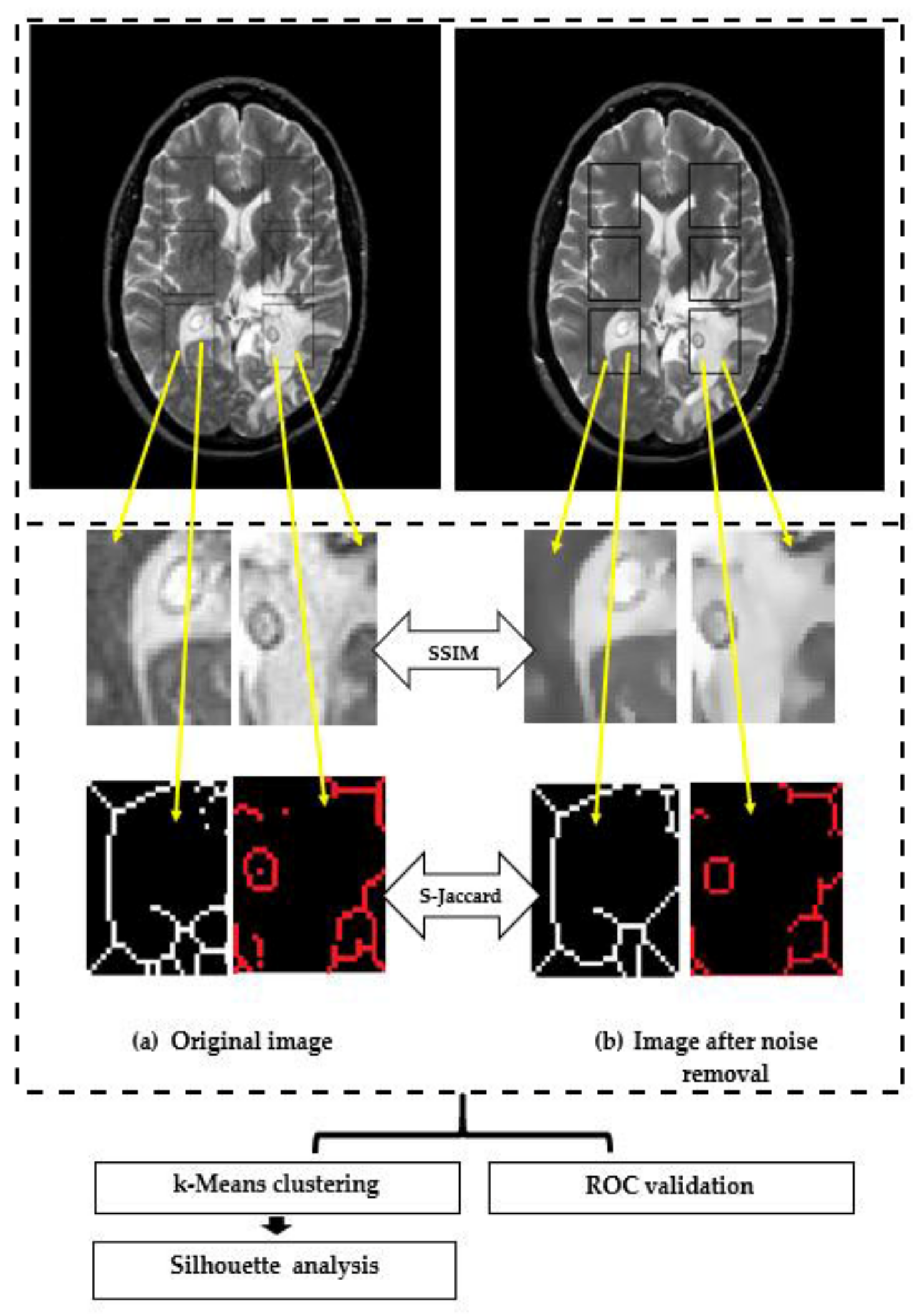
The flow chart of post-processing and analysis is shown in Figure 1.
The following steps were performed:
- Two datasets are generated: D1 contains raw images and D2 contains denoised images by using an anisotropic diffusion filter,
- select ROIs for further image manipulation tasks; insert and crop out the rectangle ROIs with a size of 35 × 45 pixels. This consisted of:
- (i)
- design the first rectangle mask in the right hemisphere,
- (ii)
- determine the distances to generate the other two rectangle masks in the right hemisphere,
- (iii)
- insert the other two masks into the right hemisphere according to the distances from step (ii),
- (iv)
- perform the mirror reflection of the masks into the right hemisphere onto the left hemisphere.
- crop out ROIs from both hemispheres, following the algorithm of step (II),
- compute SSIM for monochrome ROIs,
- segment ROIs with the skeleton algorithm,
- calculate S-Jaccard for ROIs processed in step (V),
- carry out a k-means clustering over SSIM and S-Jaccard values and pathologies,
- carry out cluster analysis with the silhouette method.
- carry out classification data using ROC analysis.
Both metrics (i.e., SSIM and S-Jaccard) were computed in every possible pair pathology-image type. For each dataset, 264 pairs were analyzed which belong to ROIs having the same spatial coordinates for all the studied images.
3. Results
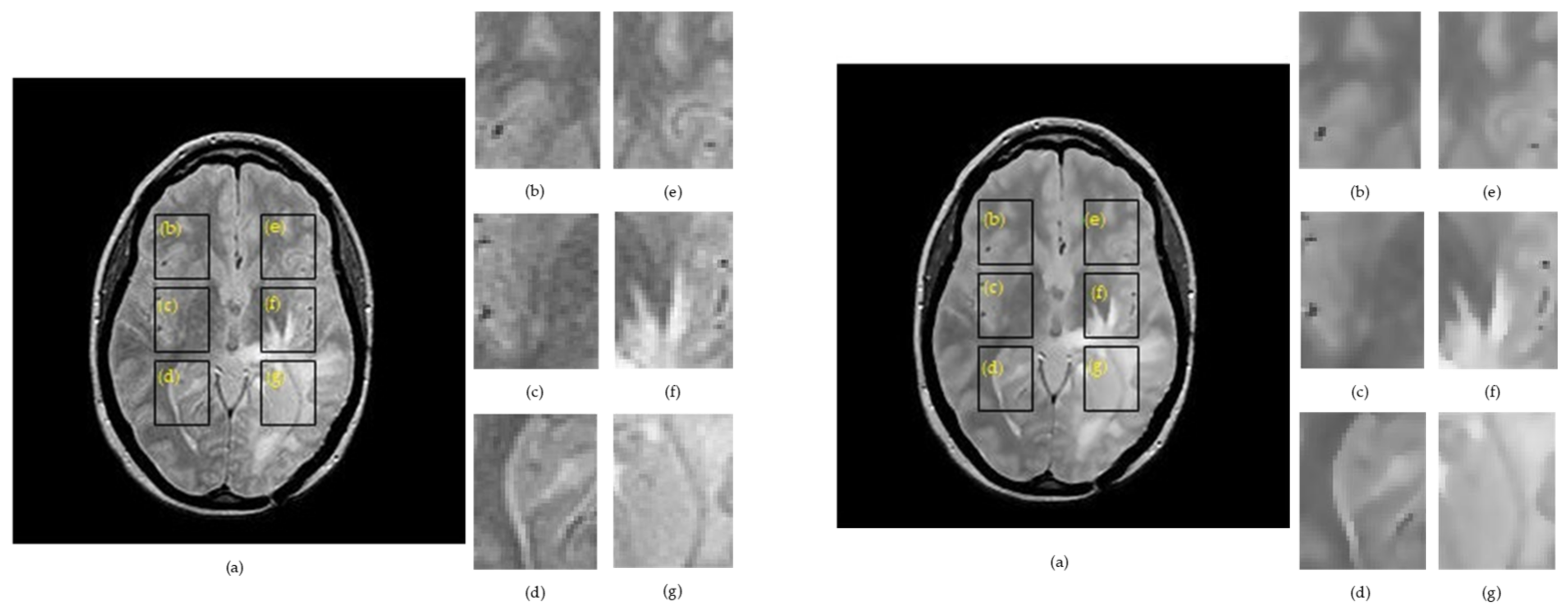
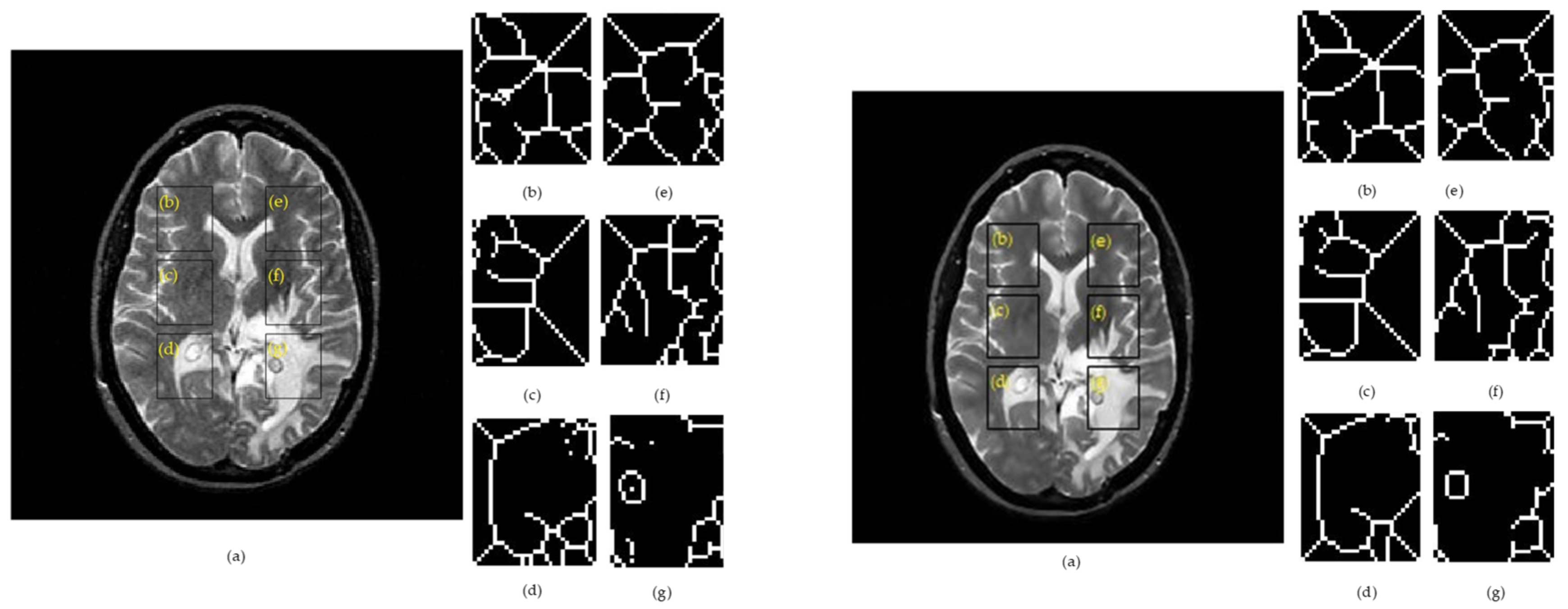
Figure 2 and Figure 3 show examples for the implementation of SSIMs and skeletonization for right– left correspondents for a raw image containing Rician noise (left panel) and a filtered image by the anisotropic diffusion filter (right panel).
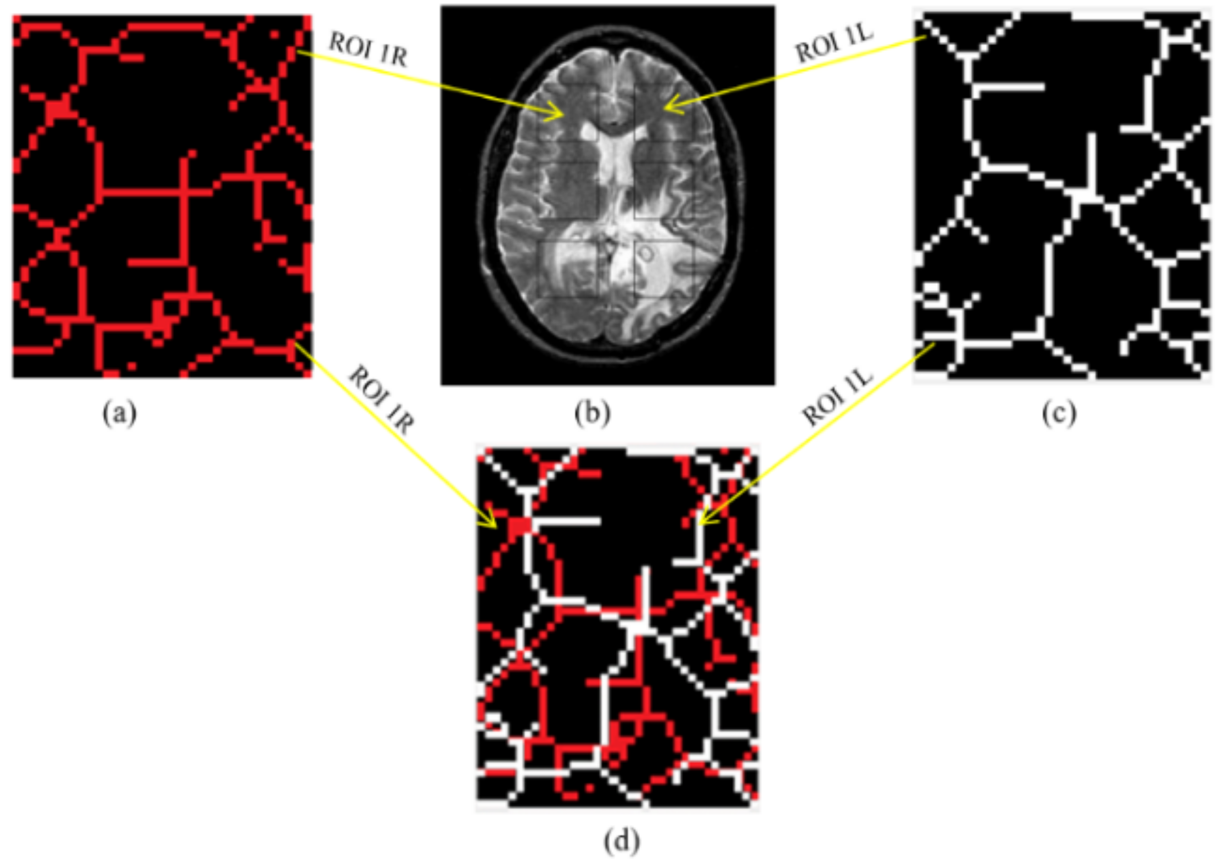
The region of interests cut from the right hemisphere were labelled as ROI 1R, ROI 2R, ROI 3R, and their symmetry in the left hemisphere were denoted as ROI 1L, ROI 2L, ROI 3L. Figure 4 summarizes the skeletonization results for a patient with glioma by providing a direct comparison of the morphological skeleton transform between brain hemispheres. The skeletal maps for two correlated ROIs were overlapped to provide a facile evaluation of dissimilarities.
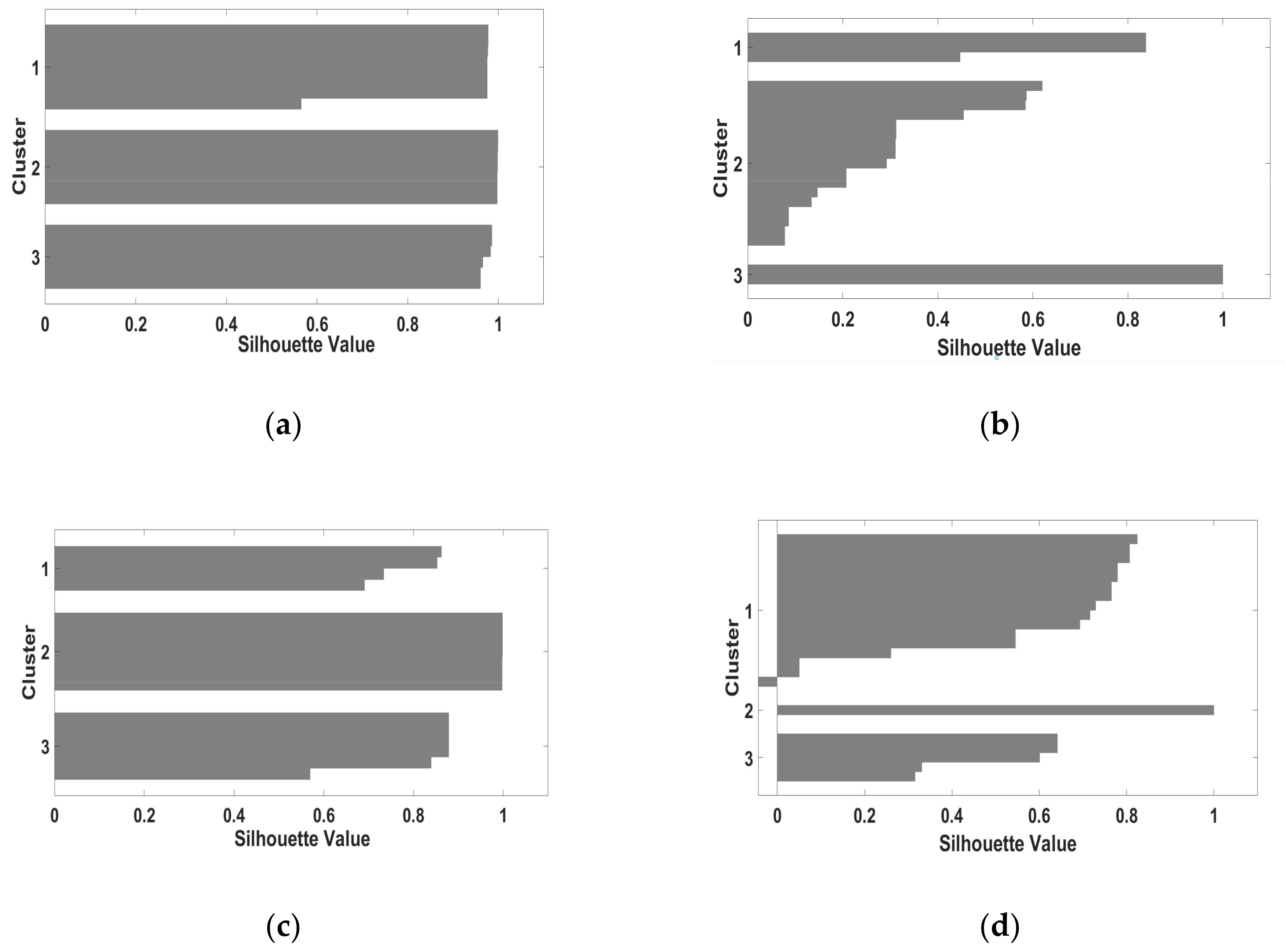
The k-mean clustering algorithm was used to group the n observations (i.e., SSIM and S-Jaccard values) into clusters. The Silhouette method assessed the relative quality of the clusters and provided information on the data configuration and clustering validity and the results for S-Jaccard are shown in Figure 5 and Figure 6. We have to mention that the number of clusters k = 3 follows the number of S-Jaccard 1 (between ROI 1R and its mirror symmetric ROI 1L), S-Jaccard 2 (between ROI 2R and its mirror symmetric ROI 2L) and S-Jaccard 3 (between ROI 3R and its mirror symmetry ROI 3L).
Figure 5 and Figure 6 containing the silhouette structure of S-Jaccard for both datasets D1, and D2 show the two cases of negative clusters (glioma/T2w, glioma/PD). Thus, for glioma/PD case S(i) = −0.45 and for glioma/T2w case S(i) = −0.1, and SSIM_ glioma/ T2w is characterized by S(i) = −0.05 indicating an intermediate case lying far from the other two clusters or that analyzed objects are dispensed to another close cluster. However, for denoised images these negative clusters are substantially reduced. Also, data in Table 1 indicate a clear-cut clusters structure. There are two exceptions for SSIM_ glioma/PD and S-Jaccard_glioma/T2w for noisy images in D1. Moreover, data in Table 1 shows a slightly weak performance for PD images for both pathologies, as the silhouette coefficient is 10%–15% lower than SC corresponding to the T2w images. Nevertheless, the SC values in Table 1 indicate a dominant strong (well-defined) cluster structure. In this comparison, a better clustering performance was achieved when a denoising operation was carried out (results for database D2).
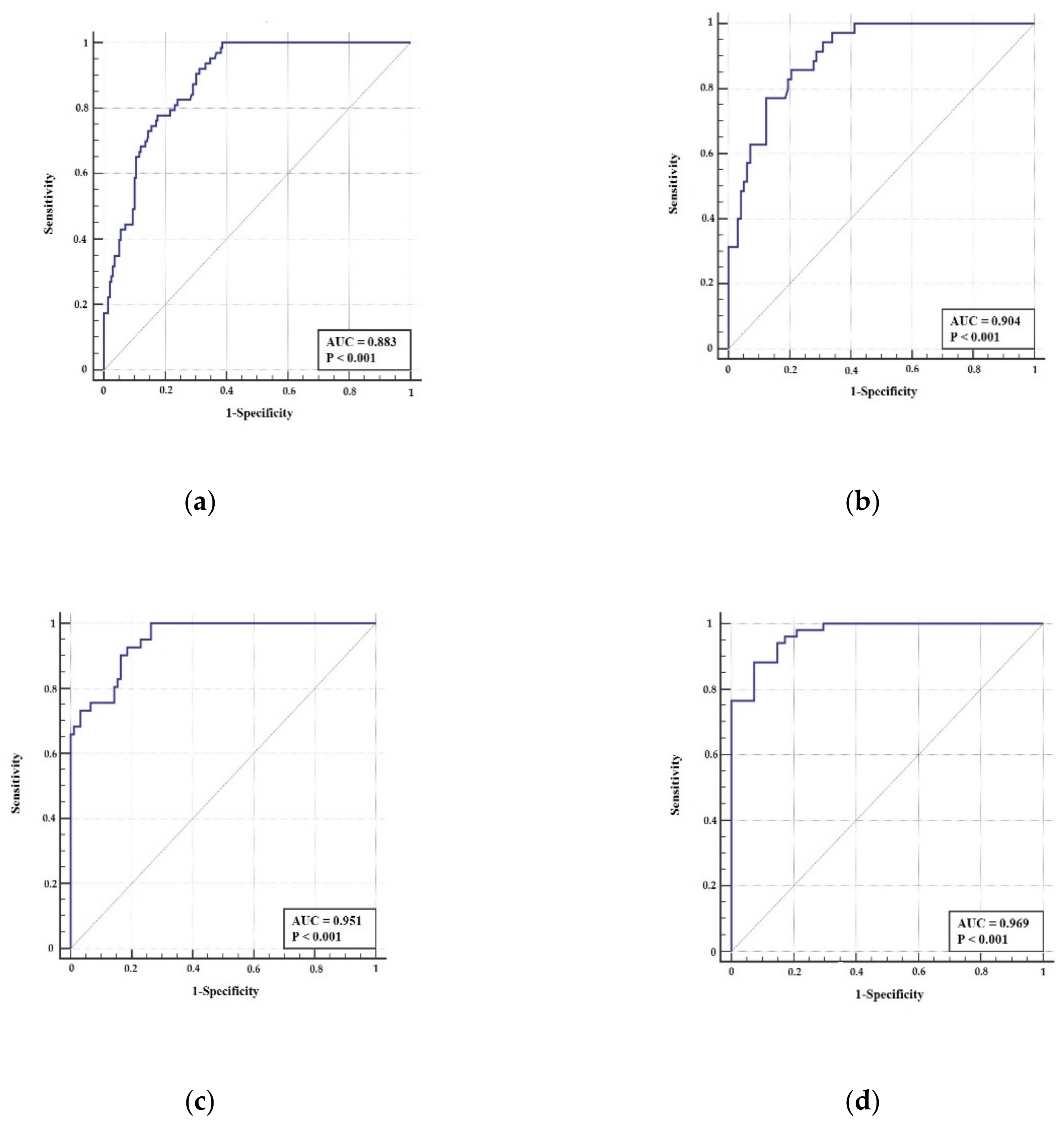
Figure 7 illustrates the ROC curves for both cases: raw and denoised images. It shows that the skeletonization accuracy, which is smaller for original images, affected by the Rician noise, where the obtained AUC is 0.883, and 0.904 with the T2w, and PD, images, respectively. However, the accuracy increases in the denoised images showing AUC 0.951, and 0.969 with T2w, and PD images, respectively. The average SNR is 18.5 dB for T2w images, and 14.72 dB for PD images. Since both the SC and AUC values for the S-Jaccard index are high for the images in D2, it can be concluded that the edges are preserved and there are no artifacts generated during the denoising operation. Also, the point closest-to-(0, 1) corner (ER) is computed by minimizing the Euclidean distance between the ROC curve, and the point of intersection of the (1-specificity) axis, and sensitivity axis [30]. The ER characterizes the optimal condition when most of the individuals are classified correctly. The performance measure ER ensures both high sensitivity and specificity. Table 2 shows the cut-points ER, and the related sensitivity/specificity values. The case of glioma denoised PD images meet the condition, where the sensitivity and specificity values are almost equal to the AUC value. The average SNR is 18.5 dB for T2w images, and 14.72 dB for PD images. As the SC, AUC, and ER values for the S-Jaccard index are higher for images in D2 it can be concluded that the edges are preserved and there are no artifacts generated during the denoising process.
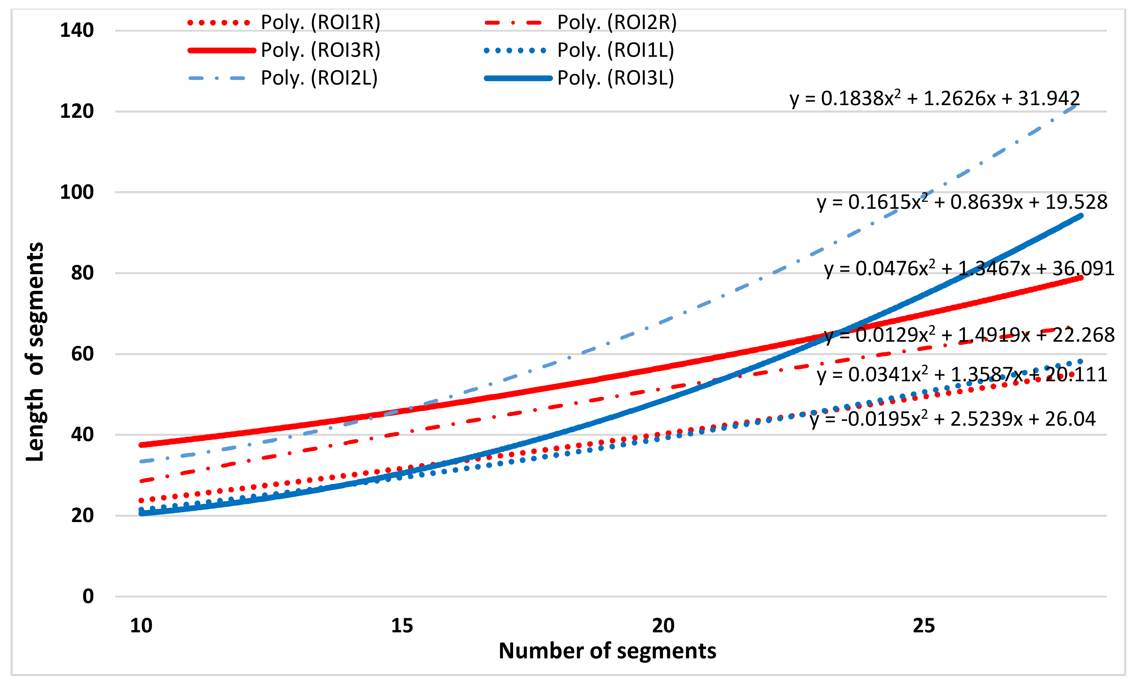
The trend lines for each analyzed ROI were determine based on the length of each skeleton segment (Figure 8 and Figure 9). A pair comparison between the left and right ROI skeleton map was empirical performed using the polynomial trend curves. As can be seen in Figure 7 and Figure 8, polynomial trend curves allow an easier detection of the dissimilarity of skeleton maps. The number of skeletal segments is highly increased for PD images compared to T2w, i.e., the edges are better preserved in PD brain images and the pattern of the trend lines is different.
4. Discussion
Several studies have been conducted on brain segmentation and classification and different applications [31,32]. In addition, skeleton transform is a quite effective and accurate approach for similarity investigations when images show a little contrast and the main cerebral tissues (i.e., gray matter, white matter, and cerebrospinal fluid) are overlapped. Experimental data analysis reveals different clustering options for SSIM and S-Jaccard provided by the Silhouette method. In this case, we focused on a cluster validity examination. Optimal clustering operation requires clusters sharing almost the same diameter and showing clearer compactness and separation. In our experiments, due to the heterogenous data of patients diagnosed with glioma, clusters may drastically be non-uniform. S-Jaccard–glioma/PD and S-Jaccard–glioma/T2w show clusters with the smallest average silhouette width (Figure 6b,d). These two extreme cases indicate a high variability of the S-Jaccard values and show the structural dissimilarity of the cerebral tissue between hemispheres in glioma patients. These results are improved by using denoised images. For healthy patients, a more uniform distribution of the clusters indicates a higher textural similarity between hemispheres. Data in Table 1 provides SC values between 0.8 and 1 indicating that a division into k = 3 clusters is a natural choice. The SC values were improved for D2. Also, the ROC and AUC accuracy improved from 0.883 to 0.951 (T2w) and from 0.904 to 0.969 (PD), respectively, when noise was removed from images. We note that that proposed algorithm provides good results for raw images (with only one exception) and substantially better results are obtained for denoised images. Data in Table 2 shows the cut-points ER and related sensitivity and specificity values. The higher sensitivity (=1) induces a detection bias as the AUC is 0.833 (case of D1, raw T2w images) The sensitivity and specificity values are almost equal to the AUC value for glioma PD images and led to the best results for our approach.
A new empirical approach was conducted with focus on skeletal similarity. The skeletons generated from the tumoral areas and the reference healthy brain were compared using the scatter plots displaying the relationship between the length of each skeletal segment and the number of segments having the same length. The trend lines for each pair of analyzed ROIs were approximated using the second-degree polynomial functions. This approach explores the visual similarity. The number of skeleton segments for PD-weighted images was higher, indicating the effectiveness of the skeletonization PD-weighted image type and the utility of the skeletonization method for segmentation. The difference between ROI pairs was empirically evaluated and indicates that visual dissimilarity is better perceived. The results of this skeletal similarity approach were compared with SSIM and S-Jaccard evaluation metrics and we reached the same conclusion, the PD-weighted image type is a better approach when the analysis is focused on edge detection.
5. Conclusions
To evaluate the textural similarity between brain hemispheres, two MRI image types (PD and T2w) for glioma and healthy patients were analyzed. The results were compared with denoised data. A morphological skeleton algorithm and a k-means clustering algorithm were used to cluster the SSIM and S-Jaccard metrics and to assess the structural similarity between brain hemispheres. Both the validity and the performance of the clustering algorithm were assessed using the silhouette score. The experimental results indicate that SSIM is independent of the texture variability while S-Jaccard is more sensitive to texture irregularities. The overall classification accuracy was assessed by ROC curve implementation. Also, a skeletal similarity empirical method using the comparison of the trend lines of skeleton map datasets indicated the PD-weighted image type as a better approach when the analysis was focused on edge detection, as it is suitable for very satisfactory edge-preserving results. At this stage of the study, S-Jaccard could be successfully used to differentiate healthy patients from those diagnosed with glioma. The proposed approach proved its efficiency as reported in the results section; accordingly, it is recommended to compare our proposed method with other studies on the evaluation of the brain tissue between hemispheres. It is also suggested to test other datasets. Our future work will investigate different brain disorders and will aim to improve the proposed method.
Author Contributions
L.M.: Research project—Conception, Organization, and Execution; Statistical Analysis—Design, Execution, Review and Critique; Manuscript—Writing of the first draft, Review and Critique. L.P.: Research project—Organization and Execution; Statistical Analysis—Design, Review and Critique. S.M.: Research project—Conception, Organization and Execution; Software validation. N.D.: Research project—Software validation; Manuscript—Review and Critique. A.S.A.: Writing—Review & Critique and Editing. All authors have read and agreed to the published version of the manuscript.
Funding
This research received no external funding.
Conflicts of Interest
The authors declare no conflict of interest.
References
- Kumar, V.D.; Krishniah, V.V.J.R. Segmentation of Brain Tumor Using K-Means Clustering Algorithm. J. Eng. Appl. Sci. 2018, 13, 3942–3945. [Google Scholar]
- Raja, N.S.M.; Fernandes, S.L.; Dey, N.; Satapathy, S.C.; Rajinikanth, V. Contrast enhanced medical MRI evaluation using Tsallis entropy and region growing segmentation. J. Ambient. Intell. Hum. Comput. 2018, 1–12. [Google Scholar] [CrossRef]
- Dey, N.; Rajinikanth, V.; Shi, F.; Tavares, J.M.R.; Moraru, L.; Karthik, K.A.; Lin, H.; Kamalanand, K.; Emmanuel, C. Social-Group-Optimization based tumor evaluation tool for clinical brain MRI of Flair/diffusion-weighted modality. Biocybern. Biomed. Eng. 2019, 39, 843–856. [Google Scholar] [CrossRef] [Green Version]
- Rajinikanth, V.; Dey, N.; Satapathy, S.C.; Ashour, A.S. An approach to examine magnetic resonance angiography based on Tsallis entropy and deformable snake model. Future Gener. Comput. Syst. 2018, 85, 160–172. [Google Scholar] [CrossRef]
- Rajinikanth, V.; Satapathy, S.C.; Dey, N.; Lin, H. Evaluation of ischemic stroke region from CT/MR images using hybrid image processing techniques. In Intelligent Multidimensional Data and Image Processing; IGI Global: Hershey, PL, USA, 2018; pp. 194–219. [Google Scholar] [CrossRef]
- Brem, S.; Abdullah, K.G. Glioblastoma E-Book, 1st ed.; Elsevier Health Sciences: Philadelphia, PA, USA, 2016. [Google Scholar]
- Sharma, K.; Virmani, J. A decision support system for classification of normal and medical renal disease using ultrasound images: A decision support system for medical renal diseases. Int. J. Ambient Comput. Intell. 2017, 8, 52–69. [Google Scholar] [CrossRef]
- Moldovanu, S.; Moraru, L.; Biswas, A. Edge-Based Structural Similarity Analysis in Brain MR Images. J. Med. Imaging Health Inf. 2016, 6, 539–546. [Google Scholar] [CrossRef]
- Tian, F.; Hayano, K.; Kambadakone, A.R.; Sahani, D.V. Response assessment to neoadjuvant therapy in soft tissue sarcomas: Using CT texture analysis in comparison to tumor size, density, and perfusion. Abdom Imaging 2015, 40, 1705–1712. [Google Scholar] [CrossRef]
- Nachimuthu, D.S.; Baladhandapani, A. Multidimensional Texture Characterization: On Analysis for Brain Tumor Tissues Using MRS and MRI. J. Digit. Imaging 2014, 27, 496–506. [Google Scholar] [CrossRef] [PubMed] [Green Version]
- Moraru, L.; Moldovanu, S.; Dimitrievici, L.T.; Ashour, A.S.; Dey, N. Texture anisotropy technique in brain degenerative diseases. Neural Comput. Appl. 2018, 30, 1667–1677. [Google Scholar] [CrossRef]
- Dewi, C. Clustering of high resolution UAV imagery to identify essential plants using some neural network. J. Env.. Eng. Sustain. Technol. 2017, 4, 55–63. [Google Scholar]
- Niwattanakul, S.; Singthongchai, J.; Naenudorn, E.; Wanapu, S. Using of Jaccard Coefficient for Keywords Similarity. In Proceedings of the International Multiconference of Engineers and Computer Scientists, Hong Kong, 13–15 March 2013; Volume 1. [Google Scholar]
- Lee, T.-C.; Kashyap, R.L. Building skeleton models via 3-D medial surface axis thinning algorithms. CVGIP Graph. Models Image Process. 1994, 56, 462–478. [Google Scholar] [CrossRef]
- Yang, X.; Zhanghao, K.; Wang, H.; Liu, Y.; Wang, F.; Zhang, X.; Shi, K.; Gao, J.; Jin, D.; Xi, P. Versatile application of fluorescent quantum dot labels in super-resolution fluorescence microscopy. ACS Photonics 2016, 9, 1611–1618. [Google Scholar] [CrossRef]
- Wu, Y.; Zhao, Z.; Wu, W.; Lin, Y.; Wang, M. Automatic glioma segmentation based on adaptive superpixel. BMC Med. Imaging 2019, 19, 73. [Google Scholar] [CrossRef] [PubMed] [Green Version]
- Zhao, Z.; Yang, G.; Lin, Y.; Pang, H.; Wang, M. Automated glioma detection and segmentation using graphical models. PLoS ONE 2018, 22. [Google Scholar] [CrossRef] [PubMed] [Green Version]
- Yang, Z.; Guo, F.; Dong, P. Robust skeleton extraction of gray images based on level set approach. J. Multimedia 2013, 8, 24–31. [Google Scholar] [CrossRef]
- Shen, W.; Zhao, K.; Jiang, Y.; Wang, Y.; Zhang, Z.; Bai, X. Object skeleton extraction in natural images by fusing scale-associated deep side outputs. In In Proceedings of the IEEE Conference on Computer Vision and Pattern Recognition (CVPR), Las Vegas, NV, USA, 27–30 June 2016; pp. 222–230. [Google Scholar]
- Soille, P. Morphological Image Analysis: Principles and Applications, 2nd ed.; Springer: Berlin/Heidelberg, Germany, 2004. [Google Scholar]
- Wang, S.; Geng, Z.; Zhang, J.; Chen, Y.; Wang, J. A Fuzzy C-means Model Based on the Spatial Structural Information for Brain MRI Segmentation. Int. J. Signal. Process. Image Process. Pattern Recognit. 2014, 7, 313–322. [Google Scholar] [CrossRef] [Green Version]
- Kertels, O.; Linsenmann, T.; Kessler, A.F.; Kircher, M.; Brumberg, J.; Tran-Gia, J.; Malte, K.; Joachim, B.; Maria, M.C.; Samuel, S.; et al. Clinical utility of different approaches for detection of late pseudoprogression in glioblastoma with O-(2-[18F]fluoroethyl)-L-tyrosine PET. Nuklearmedizin 2019, 58, 174–175. [Google Scholar]
- Buades, A.; Coll, B.; Morel, J.-M. Computer vision and pattern recognition. In In Proceedings of the CVPR IEEE Computer Society Conference on IEEE, IEEE. San Diego, CA, USA, 20–26 June 2005; pp. 60–65. [Google Scholar]
- Pal, C.; Das, P.; Chakrabarti, A.; Ghosh, R. Rician noise removal in magnitude MRI images using efficient anisotropic diffusion filtering. Int. J. Imaging Syst. Technol. 2017, 27, 248–264. [Google Scholar] [CrossRef]
- Anoraganingrum, D. Cell segmentation with median filter and mathematical morphology operation. In Proceedings of the 10th International Conference on Image Analysis and Processing, Venice, Italy, 27–29 September 1999; pp. 1043–1047. [Google Scholar]
- Moraru, L.; Moldovanu, S.; Dimitrievici, L.T.; Dey, N.; Ashour, A.S.; Shi, F.; Fong, S.J.; Khan, S.; Biswas, A. Gaussian mixture model for texture characterization with application to brain DTI images. J. Adv. Res. 2019, 16, 15–23. [Google Scholar] [CrossRef]
- Jain, A.K. Data clustering: 50 years beyond K-means. Pattern Recognit Lett. 2010, 31, 651–666. [Google Scholar] [CrossRef]
- Rousseeuw, P.J. Silhouettes: A graphical aid to the interpretation and validation of cluster analysis. J. Comput. Appl. Math. 1987, 20, 53–65. [Google Scholar] [CrossRef] [Green Version]
- Johnson, K.A.; Becker, J.A. Available online: http://www.med.harvard.edu/AANLIB/ (accessed on 7 March 2020).
- Dong, T.; Attwood, K.; Hutson, A.; Liu, S.; Tian, L. A new diagnostic accuracy measure and cut-point selection criterion. Stat. Methods Med. Res. 2017, 26, 2832–2852. [Google Scholar] [CrossRef] [PubMed]
- Ali, M.N.Y.; Sarowar, M.G.; Rahman, M.L.; Chaki, J.; Dey, N.; Tavares, J.M.R. Adam deep learning with SOM for human sentiment classification. Int. J. Ambient Comput. Intell. 2019, 10, 92–116. [Google Scholar] [CrossRef] [Green Version]
- Xiong, D.; Yan, L. A Classification Learning Research based on Discriminative Knowledge-Leverage Transfer. Int. J. Ambient Comput. Intell. 2018, 9, 52–68. [Google Scholar] [CrossRef] [Green Version]
Figure 1.
The proposed post-processing and analysis.

Figure 2.
Example of extracting regions of interes ROIs in proton density PD image for a patient with glioma, where: Left side: (a) raw image. Right side: (a) denoised image. (b) ROI 1L; (c) ROI 2L; (d) ROI 3L; (e) ROI 1R; (f) ROI 2R; and (g) ROI 3R.
Figure 2.
Example of extracting regions of interes ROIs in proton density PD image for a patient with glioma, where: Left side: (a) raw image. Right side: (a) denoised image. (b) ROI 1L; (c) ROI 2L; (d) ROI 3L; (e) ROI 1R; (f) ROI 2R; and (g) ROI 3R.

Figure 3.
Results of the skeleton algorithm for a T2w image belonging to a patient with glioma, where: Left side: (a) raw image. Right side: (a) denoised image. (b) ROI 1L; (c) ROI 2L; (d) ROI 3L; (e) ROI 1R; (f) ROI 2R; and (g) ROI 3R.
Figure 3.
Results of the skeleton algorithm for a T2w image belonging to a patient with glioma, where: Left side: (a) raw image. Right side: (a) denoised image. (b) ROI 1L; (c) ROI 2L; (d) ROI 3L; (e) ROI 1R; (f) ROI 2R; and (g) ROI 3R.

Figure 4.
(a) Skeletal map of ROI 1R; (b) rectangular masks overlaid on a T2w MRI image for a patient diagnosed with glioma; (c) Skeletal map of ROI 1L; (d) ROI 1R, and ROI 1L overlapped to highlight differences between the skeletal maps.
Figure 4.
(a) Skeletal map of ROI 1R; (b) rectangular masks overlaid on a T2w MRI image for a patient diagnosed with glioma; (c) Skeletal map of ROI 1L; (d) ROI 1R, and ROI 1L overlapped to highlight differences between the skeletal maps.

Figure 5.
Cluster validity for S-Jaccard values for raw images belonging to D1. The name of the images follows the pattern: Diagnose Index/MRI image type. (a) S-Jaccard_ healthy/T2w; (b) S-Jaccard_ glioma/ T2w; (c) S-Jaccard_ healthy/PD; (d) S-Jaccard_ glioma/ PD.
Figure 5.
Cluster validity for S-Jaccard values for raw images belonging to D1. The name of the images follows the pattern: Diagnose Index/MRI image type. (a) S-Jaccard_ healthy/T2w; (b) S-Jaccard_ glioma/ T2w; (c) S-Jaccard_ healthy/PD; (d) S-Jaccard_ glioma/ PD.

Figure 6.
Cluster validity for S-Jaccard values for denoised images belonging to D2. The name of the images follows the pattern: Diagnose Index/MRI image type. (a) S-Jaccard_ healthy /T2w; (b) S-Jaccard_ glioma/T2w; (c) S-Jaccard_ healthy /PD; (d) S-Jaccard_ glioma /PD.
Figure 6.
Cluster validity for S-Jaccard values for denoised images belonging to D2. The name of the images follows the pattern: Diagnose Index/MRI image type. (a) S-Jaccard_ healthy /T2w; (b) S-Jaccard_ glioma/T2w; (c) S-Jaccard_ healthy /PD; (d) S-Jaccard_ glioma /PD.

Figure 7.
ROC curves for S-Jaccard computed for glioma images in D1 dataset (top) and D2 dataset (bottom), (a) raw T2w image, (b) raw PD image, (c) denoised T2w image, and (d) denoised PD image.
Figure 7.
ROC curves for S-Jaccard computed for glioma images in D1 dataset (top) and D2 dataset (bottom), (a) raw T2w image, (b) raw PD image, (c) denoised T2w image, and (d) denoised PD image.

Figure 8.
Fitted curves on number of skeleton segments vs. length of the segments (i.e., the corresponding connected pixels) for T2-weighted image for a patient with glioma.
Figure 8.
Fitted curves on number of skeleton segments vs. length of the segments (i.e., the corresponding connected pixels) for T2-weighted image for a patient with glioma.

Figure 9.
Fitted curves on number of skeleton segments vs. length of the segments (i.e., the corresponding connected pixels) for PD-weighted image for a patient with glioma.
Figure 9.
Fitted curves on number of skeleton segments vs. length of the segments (i.e., the corresponding connected pixels) for PD-weighted image for a patient with glioma.


Table 1.
The SC values for both pathologies and MRI image type.
| Diagnosis/MRI Image Type | SSIM (Database D1) | SSIM (Database D2) | S-Jaccard (Database D1) | S-Jaccard (Database D2) |
|---|---|---|---|---|
| Healthy /T2w | 0.996 | 0.998 | 0.894 | 0.999 |
| Glioma/T2w | 0.998 | 0.998 | 0.656 | 0.999 |
| Healthy /PD | 0.953 | 0.961 | 0.881 | 0.998 |
| Glioma/PD | 0.901 | 0.921 | 0.980 | 0.991 |
Table 2.
The cut-points ER, area under the curve AUC and related sensitivity and specificity values, for S-Jaccard computed for glioma images.
Table 2.
The cut-points ER, area under the curve AUC and related sensitivity and specificity values, for S-Jaccard computed for glioma images.
| S-Jaccard | AUC | Sensitivity | Specificity | ER |
|---|---|---|---|---|
| denoised T2w image | 0.951 | 0.927 | 0.813 | 0.2 |
| denoised PD image | 0.969 | 0.882 | 0.926 | 0.139 |
| raw T2w image | 0.833 | 1 | 0.657 | 0.343 |
| raw PD image | 0.904 | 0.857 | 0.794 | 0.25 |
© 2020 by the authors. Licensee MDPI, Basel, Switzerland. This article is an open access article distributed under the terms and conditions of the Creative Commons Attribution (CC BY) license (http://creativecommons.org/licenses/by/4.0/).
Share and Cite
MDPI and ACS Style
Pana, L.; Moldovanu, S.; Dey, N.; Ashour, A.S.; Moraru, L. Brain Tissue Evaluation Based on Skeleton Shape and Similarity Analysis between Hemispheres. Computation 2020, 8, 31. https://0-doi-org.brum.beds.ac.uk/10.3390/computation8020031
AMA Style
Pana L, Moldovanu S, Dey N, Ashour AS, Moraru L. Brain Tissue Evaluation Based on Skeleton Shape and Similarity Analysis between Hemispheres. Computation. 2020; 8(2):31. https://0-doi-org.brum.beds.ac.uk/10.3390/computation8020031
Chicago/Turabian StylePana, Lenuta, Simona Moldovanu, Nilanjan Dey, Amira S. Ashour, and Luminita Moraru. 2020. "Brain Tissue Evaluation Based on Skeleton Shape and Similarity Analysis between Hemispheres" Computation 8, no. 2: 31. https://0-doi-org.brum.beds.ac.uk/10.3390/computation8020031
Note that from the first issue of 2016, this journal uses article numbers instead of page numbers. See further details here.