Computational Analysis of Air Lubrication System for Commercial Shipping and Impacts on Fuel Consumption


Fluid Mechanics Laboratory (FML), Mechanical Engineering and Aeronautics Department, University of Patras, GR-26500 Patras, Greece
*
Authors to whom correspondence should be addressed.
Computation 2020, 8(2), 38; https://0-doi-org.brum.beds.ac.uk/10.3390/computation8020038
Submission received: 25 February 2020
/
Revised: 20 April 2020
/
Accepted: 22 April 2020
/
Published: 28 April 2020
(This article belongs to the Special Issue Selected Papers from the 8th International Conference on Experiments/Process/System Modeling/Simulation/Optimization (IC-EPSMSO 2019))
Abstract
:Our study presents the computational implementation of an air lubrication system on a commercial ship with 154,800 m3 Liquified Natural Gas capacity. The air lubrication reduces the skin friction between the ship’s wetted area and sea water. We analyze the real operating conditions as well as the assumptions, that will approach the problem as accurately as possible. The computational analysis is performed with the ANSYS FLUENT software. Two separate geometries (two different models) are drawn for a ship’s hull: with and without an air lubrication system. Our aim is to extract two different skin friction coefficients, which affect the fuel consumption and the CO2 emissions of the ship. A ship’s hull has never been designed before in real scale with air lubrication injectors adjusted in a computational environment, in order to simulate the function of air lubrication system. The system’s impact on the minimization of LNG transfer cost and on the reduction in fuel consumption and CO2 emissions is also examined. The study demonstrates the way to install the entire system in a new building. Fuel consumption can be reduced by up to 8%, and daily savings could reach up to EUR 8000 per travelling day.
1. Introduction
In recent years, marine engineers and maritime companies have struggled to construct vessels with the lowest possible fuel consumption, in order to achieve the maximization of benefits and reduction of pollutants. Furthermore, rising fuel prices and restricted rules in emissions amplify the need for lower ship resistance and requisite propulsion power [1]. Each ship must face three kinds of resistance: wave, pressure and skin friction resistance. Wave and pressure resistances are inevitable and can be easily confronted by the detailed design of the hull. However, the reduction in the skin friction resistance remains proportionate to the wetted surface and the cruising speed, and even small decreases in skin friction have large impacts on the fuel consumption and the reduction of emissions [2]. Several passive methods exist which attempt to reduce friction resistance, such as specific hydrophobic dyes and nanocomposite add-ons [3]. The dominating active method for the reduction of skin friction is the injection of air into the boundary layer underneath the hull, namely air lubrication. The use of air as a lubricant has been proved analytically, experimentally and computationally to decrease the friction between the ship and the seawater.
There are three known methods of air lubrication: bubble injection, air layers and air cavities. It has been experimentally proved that bubble injection is the best method, but it is difficult to consistently create the right bubble size and maintain the bubble mattress under the hull. Air lubrication has been studied with real experiments since the 1990s. However, computational research and computing simulations of this system have not yet been widely conducted. Thus, research into this system on a real scale ship in ANSYS FLUENT is considered to be innovative and should offer useful results, combined with numerical methods.
Mr. Kodama and colleagues [4] tested the system on a plate of 50 m length, and the following tests for a single plate were accomplished into a CFD (Computational Fluid Dynamics) environment. Eventually, the air lubrication system was tested in actual scale on a newly-built ship from Mitsubishi Heavy Industries [5], called Till-Deymann. Maritime companies have started using this system in new builds. As has been proven, air lubrication contributes significantly to the performance of the ship. Therefore, there is a need for further and cheaper investigation into this system. Our study shows that a computational analysis can provide solutions and affect the evolution of air lubrication systems without demanding and expensive real tests.
Finally, taking the impact of maritime CO2 emissions into consideration, mechanisms such as air lubrication are needed. Experimental investigations have shown fuel and emission reductions of up to 8%. The CFD implementation of the air lubrication system, combined with popular numerical methods, proves the important fuel decrease.
2. Computational Analysis
We hypothesized that temperature, uninterrupted flow, draft and weight distribution along the whole length are equal and constant [6]. However, velocity, mass supply from the injectors, and hydrostatic pressure vary in the flowing field.
The ship was designed in real-time scale and two dimensions (2D), due to the lack of computational power. The length is approximately 280 m, the width almost 43 m, the mean draft 11 m, the speed 20 knots, and the injection speed 0.4 m/sec. The ship travels in full speed and is totally loaded (the service speed given by the shipowner company is 19.5 knots). The meshing of the flow-field and the optimization of the finite elements are performed using various techniques that ANSYS offers, such as inflation, edge sizing, and the quadratic cell method. These techniques guide the solver to focus and extract better results on the hull’s surface, where we are interested—this is a great advantage of the computational environment. Time is set to be transient. The interaction between the three phases (air, water, steel) is controlled using the VOF (volume of fluids) model, using explicit volume fraction parameters. Besides the VOF model, the solver used the “Viscous-Realizable k-ε” model and the “PISO” (Pressure Implicit with Splitting of Operators) scheme as solution models. The Realizable k-ε model is one of the most common turbulence models. It includes two extra transport equations to represent the turbulent properties of the flow.
The pressure-based solver used these equations to represent both the generation of turbulence kinetic energy due to the mean velocity gradients, calculated in same way as in the standard k-epsilon model, and the generation of turbulence kinetic energy due to buoyancy, calculated in same way as standard k-epsilon model. The first transported variable is turbulent kinetic energy, k. The second transported variable in this case is the turbulent dissipation, epsilon. It is the variable that determines the scale of the turbulence; whereas the first variable, k, determines the energy in the turbulence.
The “Multiphase Volume of Fluid” model was chosen, as we studied a two-phase flow (air–water) and the phases interacted without being mixed (100% v/v air cavities or bubbles were generated). Water was picked as the primary phase and air as the secondary phase.
The gravity option (on the vertical axis) was enabled, in order to take the hydrostatic pressure into consideration, as we have a hull sunken in seawater and its draught poses extra hydrostatic and hydrodynamic forces. The sea surface is simulated as a moving wall and the hull’s surface as a stationary wall with specific material properties. The computation was set to start from the left border of the flowing field (seawater inlet) and proceed to the right, simulating the cruise of the ship to the opposite direction with the same speed.
The feedback of the analysis was a phase distribution in the flowing field and the step-by-step evolution of the skin friction coefficient on the lower surface of the hull. As far as the computational calculation options are concerned, the time step size was set at 0.01 s, and the maximum number of iterations was 30.
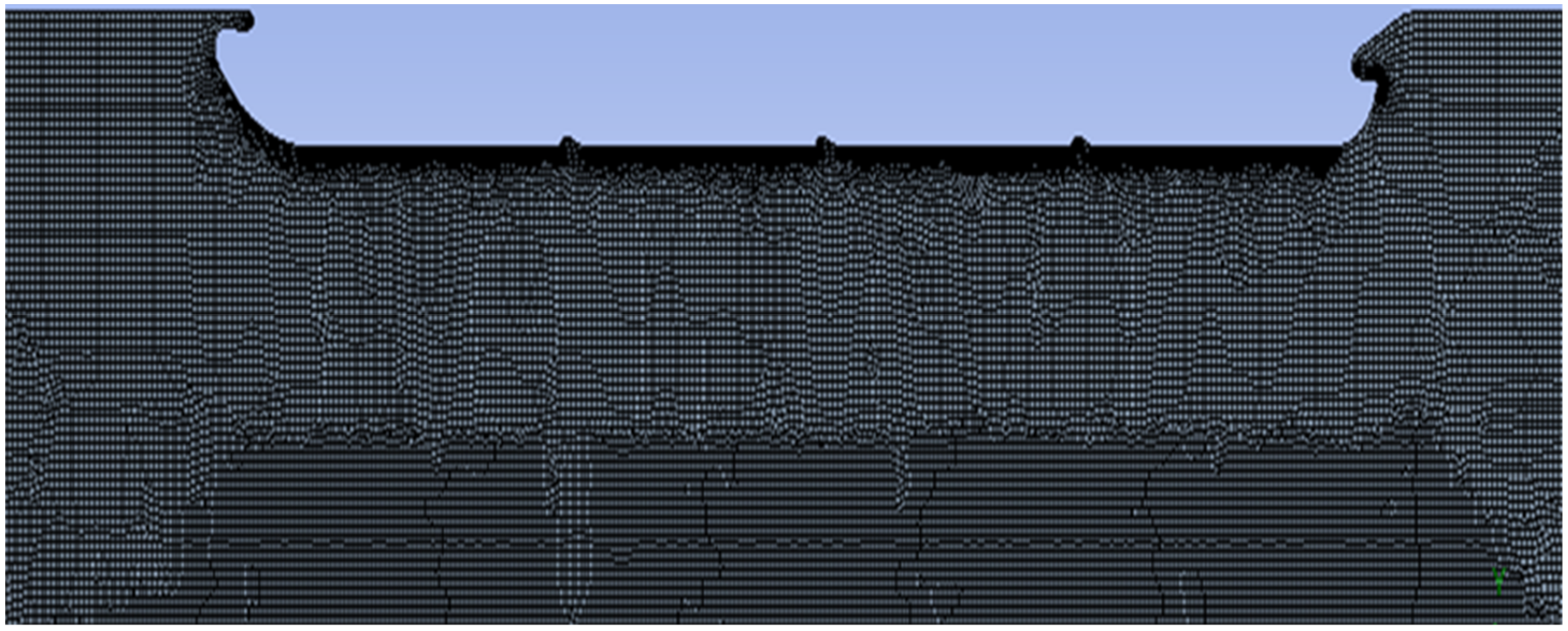
Afterwards, the solution followed a method called “Mesh-Independence” [7], because meshing affects the flow-field and the results had to have the right density. Consequently, the mesh densified up to a point where the results (e.g., skin friction coefficient) differed no more, even if the meshing was further changed. Figure 1 shows the meshed 2D flow-field for the non-air lubrication analysis. The geometry represents the design of the real ship under the sea level exactly, without the propulsion system.
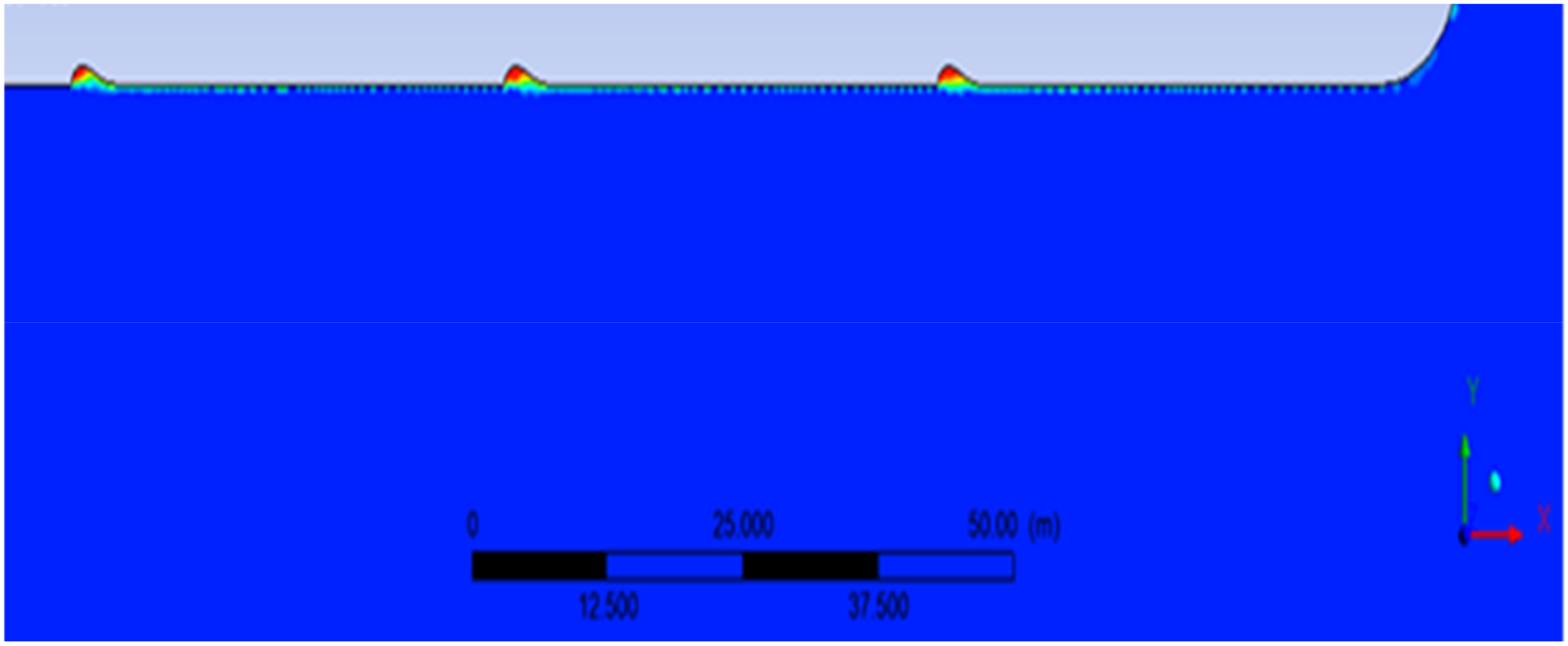
Figure 2 shows the meshing of the hull with air lubrication. Three injection zones are present and the most densified area around the hull being our area of interest. The water flow starts from the left boundary (velocity inlet).
At the no-lubrication analysis, the meshing stopped at 33,280 cells, whereas the second analysis stopped at 38,862 cells. The injectors operate as air-velocity inlets and create small air cavities or bubbles, which tend to create a bubble mattress inside the boundary layer of the hull and simultaneously reduce the hull’s skin friction coefficient.
3. Results
3.1. Results without Air Lubrication
A plain hull without air injectors and a second hull with three injection zones were created for the purposes of our study. The aim of the analysis was to extract a skin friction coefficient on the plain hull and compare it to the respective coefficient of the air-lubricated hull. The size and the geometry details in both systems were the same, except for the injectors.
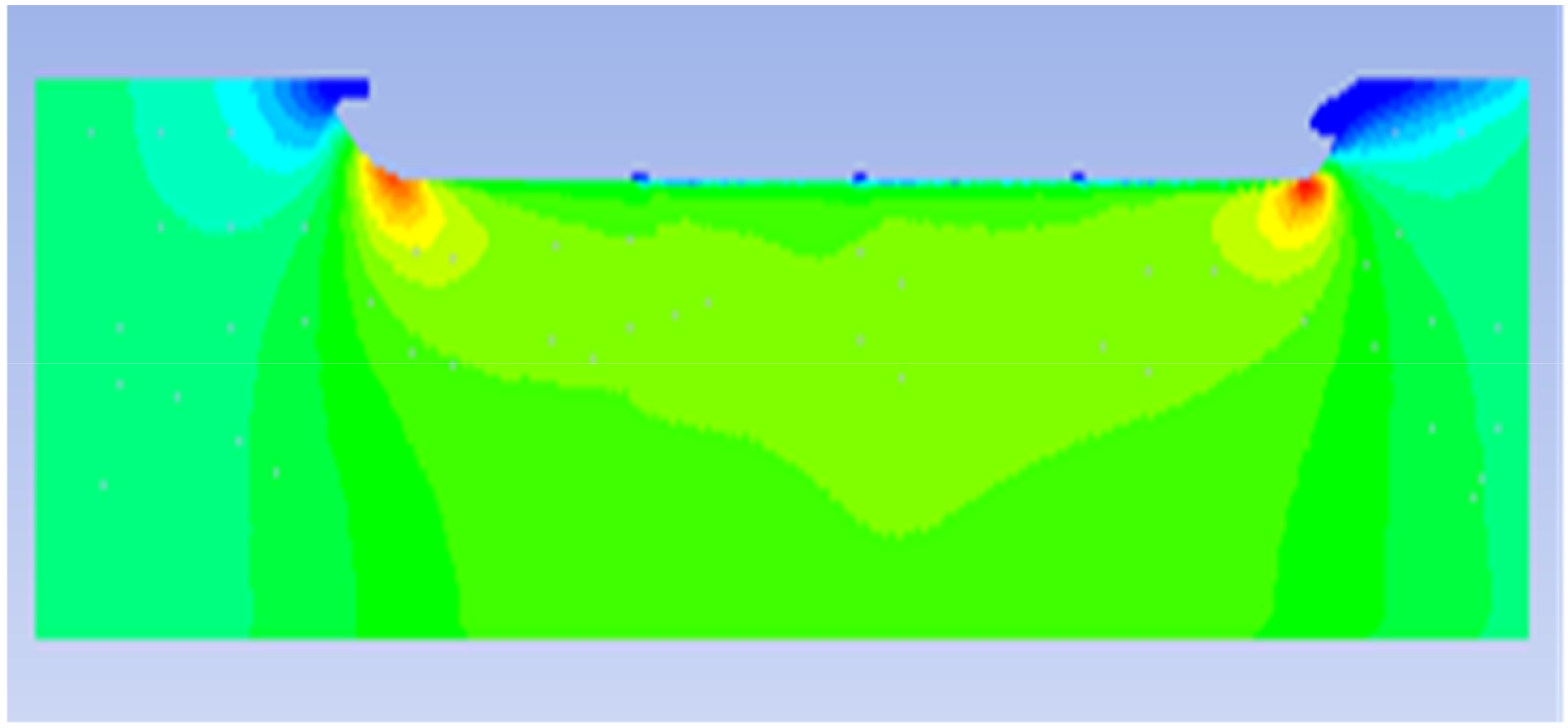
Figure 3 shows the dynamic pressure distribution, and the colors validate, that gravity and the ship’s displacement are both considered. It is important to observe the increase of dynamic pressure at specific points underneath the hull (yellow & red color) and a stable value of this pressure (green color), almost, throughout the whole length of the hull.
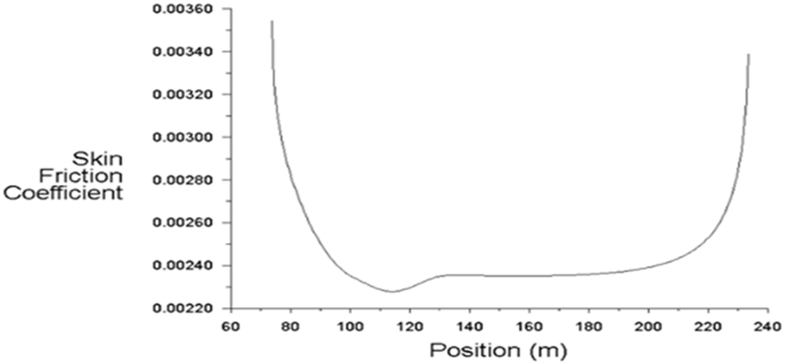
Subsequently, Figure 4 presents the distribution of the skin friction coefficient (Cf) along the hull surface. As can been seen, after 5000 time-steps, the analysis stopped and Cf was numerically stabilized at 0.0023. The hull extends from 110 m to 220 m in the graph, referring to the totally horizontal part of the bottom. Previous studies [8] agree with this value, referring to the hull’s skin friction that is in accordance with our results.
3.2. Results with Air Lubrication
The number of injection zones was chosen arbitrarily, since there are many types and formations of injectors used for air lubrication [9]. The analysis was run for over 5000 time-steps in order to let the flow evolve and be consolidated as described previously. Figure 5 projects the areas where dynamic pressure is increased and the observer can distinguish that pressure tends to decrease (blue-green color on the hull’s surface) in the air-lubricated areas compared to the no-lubricated hull.
The respective skin friction coefficient for this analysis is presented in Figure 6. The graph tends to eliminate where the seawater faces air bubbles (Cf ≈ 0), and this causes fluctuation between 0 and 0.002. Finally, the coefficient Cf (0.0020) was selected to be the upper value.
Thus, the reduction in the skin friction coefficient between the two models rises to 13%. The use of timestep animation virtualizes the flow evolution according to the selected solution options.
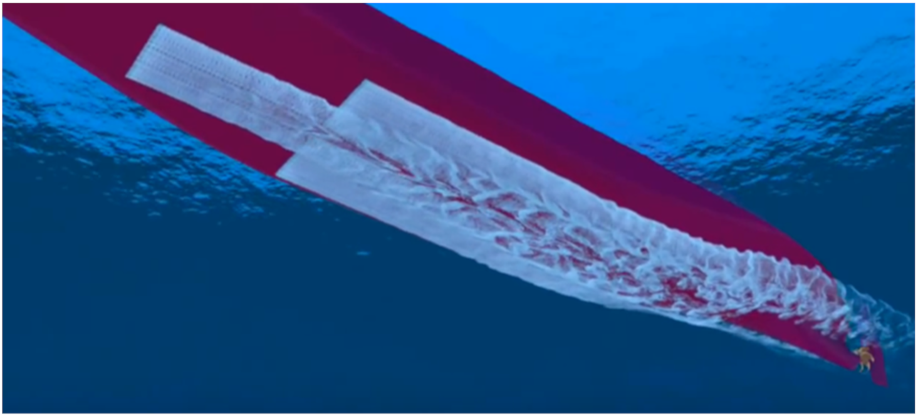
Figure 7 shows the volume fractions of air and seawater in the flow-field. The bubbles (yellow color) create a protective mattress underneath the hull as the ship cruises. Air (red color) fills the three injectors and the flow distracts small pieces of air, creating small cavities or bubbles that are attached on the hull’s surface. In that way, the skin friction coefficient is abruptly decreased, leading to a reduction in fuel consumption and emissions, as is mentioned in Section 3.
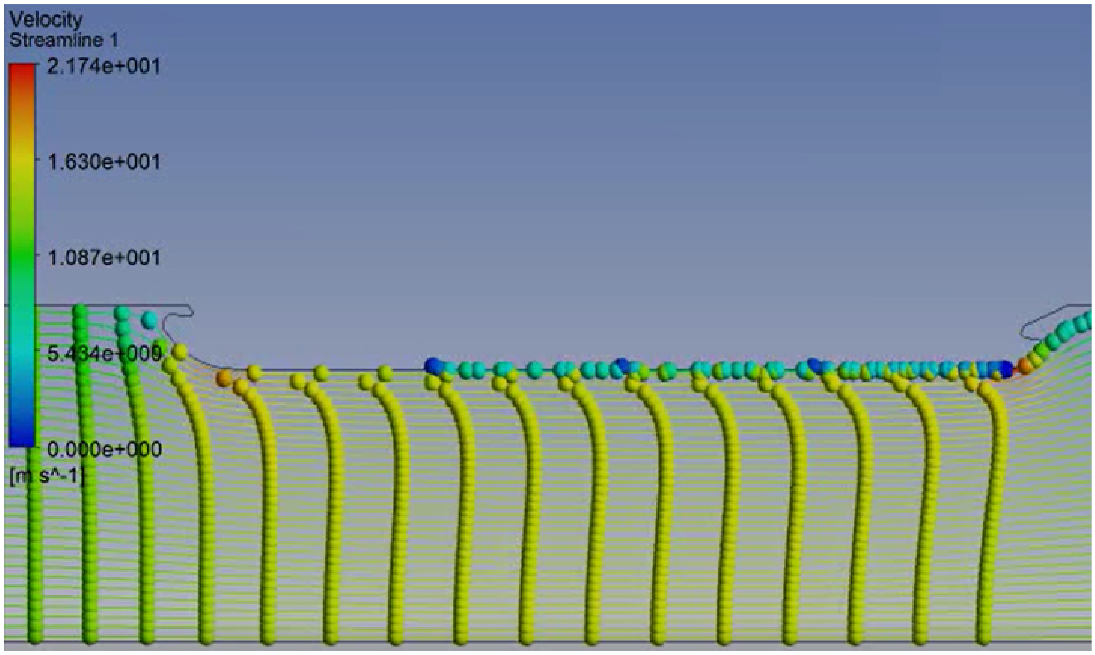
A streamline animation snapshot (Figure 8) explains the procedure, as the small air pieces (blue color) are mixed with the passing seawater flow (yellow color) at the air-lubricating areas. The flow proceeds from left to right, suggesting that the ship travels in the left direction of the flowing field.
3.3. Fuel Consumption and Emissions
Table 1 gathers the main abbreviations, in order to enhance the understanding of the following procedure.
3.3.1. Engine Features and Fuel Consumption
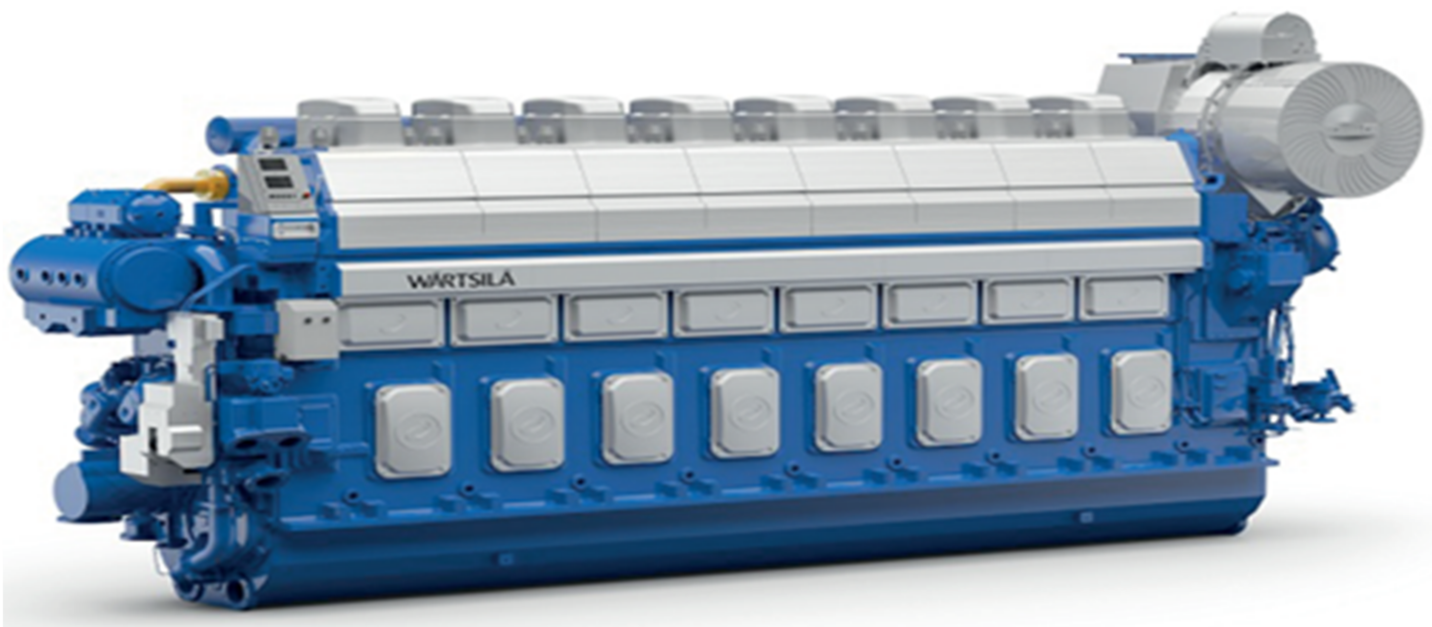
The ship, which is modelized, uses four identical engines for its propulsion. Each engine is constructed by Wartsila [10] and produces 13,740 kW at 600 rpm, using either MDO (Marine Diesel Oil) or LNG (Liquified Natural Gas), and is commonly known as Dual Fuel. Figure 9 presents this type of engine.
Nowadays, engineers tend to convert engines to operate with LNG as it is certainly cleaner and more efficient, and electro-propulsion is expected to dominate the maritime sector. The ship has 54,960 kW available propulsive power from the four engines—at least 15,000 kW more than the required power that has been calculated for the specific vessel. The primary feature for the consumption is the SFC (Specific Fuel Consumption) regarding these engines. When the ship cruises using MDO, the SFC equals to 0.160 kg/kWh.
3.3.2. Decrease in Consumption
According to naval architects [11], the total resistance coefficient is calculated using the following Equation:
CT = Cf + CA + CAA + CR
CA is the coefficient that expresses the increase in resistance due to the ship’s volume. CAA represents the air resistance coefficient, and CR is the residual resistance coefficient. For our purposes, the unknown coefficients were calculated by applying equations from the naval bibliography [12] as follows:
- CA = −0.00350,
- CAA = 0.00055,
- CR = 0.00400,
- For Cf = 0.0023 > CT = 0.00335
- For Cf = 0.0020 > CT = 0.00305 > 8.9% decrease between two CT coefficients,
Equations (2) and (3) calculate the required total propulsion resistance FT and propulsion power P accurately enough, where V represents the cruising speed, ρ the density of seawater and S the wetted surface [13].
FT = CT × 0.5 × ρ × V2 × S
P = FT × V
Having calculated the necessary variables, we can discern two cases: operation with air lubrication (YES) and without (NO). As a result, PNO = 37,862 kW and PYES = 34,474 kW. The fuel consumption (FC), using MDO in both cases, results as followed:
FCNO = SFC × PNO = 145 Tn/day
FCYES = SFC × PYES = 133 Tn/day
Importantly, the shipowner company gave the fuel consumption for this ship at service speed (19.5 knots) without air lubrication, which was equal to 142.5 tons per day. Thus, we could admit that the analysis’ results are quite accurate, considering that we posed higher cruising speed (20 knots), which means higher fuel consumption, and the fuel consumption came out at 145 tons per day. As a result, the 2.5-ton difference between the computer and reality, under the specific circumstances, is highly satisfying.
The Hellenic Petroleum s.A. gave the price of MDO (504.83 EUR/m3), and consequently, the reduction in consumption turned into economical amounts M. Using the density of MDO to control the units for each case:
MNO = 91,500 EUR/day
MYES = 83,930 EUR/day
To sum up, the usage of air lubrication reduces fuel consumption per 8% or 7500 EUR/day, as suggested by the total analysis.
3.3.3. Decrease in CO2 Emissions
The impact of air lubrication on the reduction in pollution [14] can be quantified using the following Equation (4):
Ε = FECO2 × Ch/1000 (Tn CO2/h)
E represents the amount of the produced CO2 emissions per hour, Ch is the fuel consumption in kg/h, and FECO2 is the emission coefficient of MDO. Therefore, the amount to be produced is:
ΕNO = 465 Τn/day CO2
ΕYES = 424 Τn/day CO2
Taking the price of CO2 from the stock market (12 EUR/Tn) [15], the owner is burdened in each case by:
ΜNO = 5580 EUR/day
ΜYES = 5088 EUR/day
In conclusion, the savings due to emission reduction rise by almost 500 EUR/day or 8.5%.
4. Discussion and Conclusions
4.1. Technical Remarks
Figure 10 presents the main parts, that synthesize the total air lubrication system. The operation is controlled in the automation room, where the engineer can set the variables and check the system in real time.
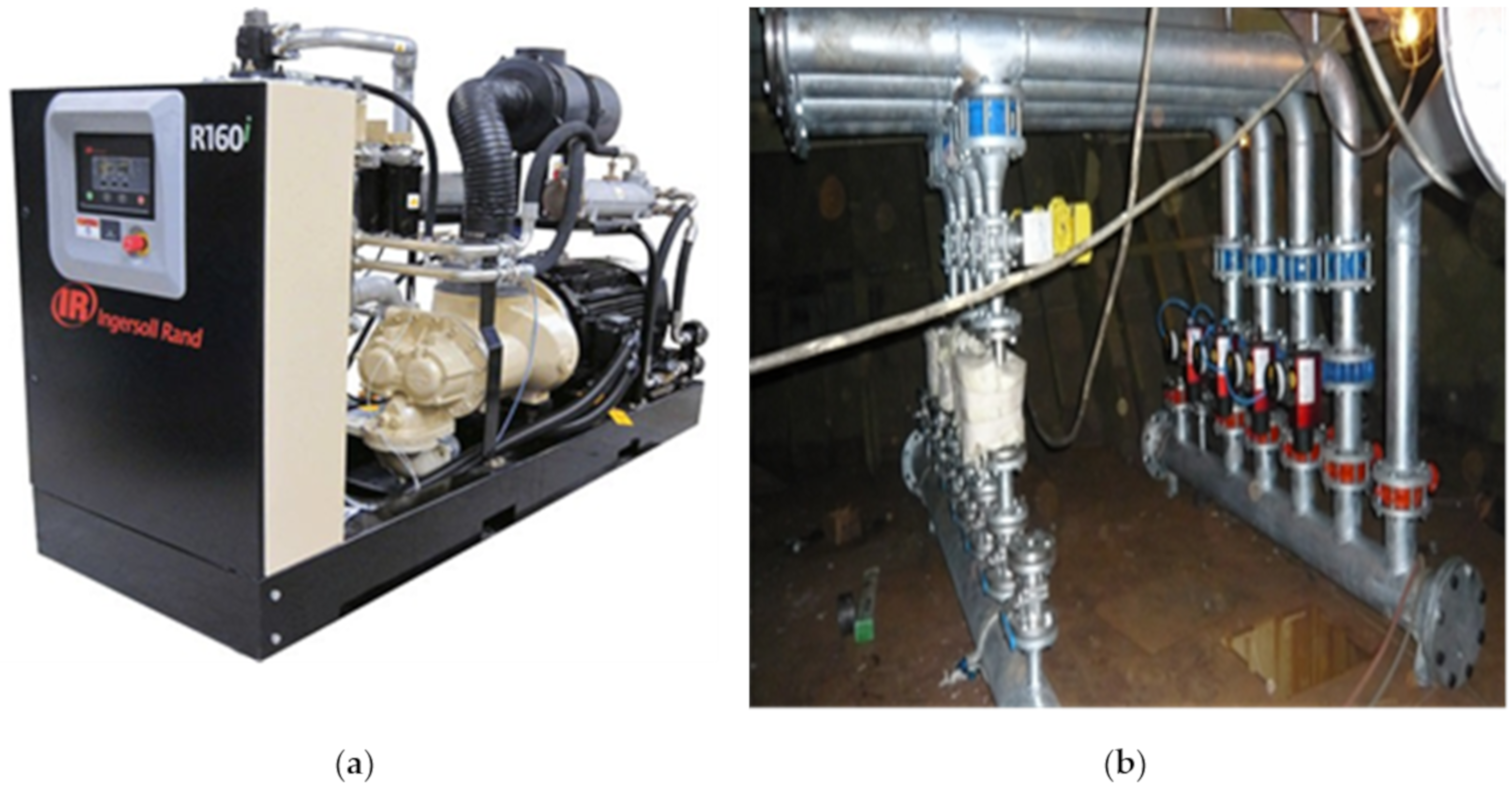
Compressors use atmospheric air and push it through the piping system to the air release units. A main pipe distributes the compressed air to smaller pipes, which end up to the injectors. An Ingersoll Rand compressor [16] with a piping installation is presented in Figure 11, and they are also suitable for the paper’s ship, as the compressor usually operates between 6 bar and 9 bar pressure, consumes 160 kW, weighs over 2 tons, and provides the piping system with maximum 27.8 m3/min of compressed air. The compressor is also seawater cooled.
The total wastage from these three main parts—and specifically the additive power—should also be taken into consideration, as well as the installation cost and the ordinary maintenance costs.
Finally, we should emphasize the importance of the injection zones and the injectors’ design. Many designer companies have created various formations and types of injectors, and this topic demands further 3D computational research in order to optimize the air injection and the bubble generation for a specific vessel.
Figure 12 and Figure 13 show the injection formations that were picked by Silverstream Technologies [17] and Mitsubishi Heavy Industries [5].
New constructors of the system try to find the right geometry for the injection zones and, certainly, the production and the research on this system can be evolved.
4.2. Conclusions
Computational analysis packages like ANSYS can give trustworthy solutions and support the research and the improvement of this system, without spending huge amounts of money on real scale tests. Despite the lack of computational power, our results are considered reliable and precise, since they follow the values of the real data given by the shipowner company.
What the specific analysis actually offers is a computational proof that the usage of air lubrication in our ship reduces the skin friction coefficient from 0.0023 to 0.0020. The computational simulation granted significant experimental information, and we were able to translate this reduction numerically into fuel and money savings (12 tons less fuel, or EUR 8000 per day). Taking into account that this ship travels unstoppably, we can assume the proportional economic and environmental benefits of air lubrication.
The operation of this system on a real ship was accurately simulated by posing the right conditions, and useful results were extracted from the virtual tools which ANSYS offers. The set-up of the analysis is claimed to be the computational decoding of air lubrication. The right settings, which simulate the procedure accurately, are discovered in this study, and this is a base for future research. We comprehended the distribution of air cavities and bubbles on the hull, the range of dynamic pressure underneath the hull and how the bubble mattress affects the cruise of the ship. The function of air lubrication and graphs of the skin friction coefficient were positively virtualized. This 2D analysis is considered to be an innovative base for the further investigation of the system.
To sum up, the computational environment gave us vulnerable data referring to skin friction resistance and bubble distribution on the hull. These data were involved, then, into numerical models, that gave us a new reduced fuel consumption. The contribution of this CFD analysis to the study of air lubrication is technologically advanced and proves that real experiments in shipyards are not compulsory anymore.
Author Contributions
A.G.F. contributed to the collection of data, writing and editing the manuscript and D.P.M. contributed to the processing of data. All authors have read and agreed to the published version of the manuscript.
Funding
This research received no external funding.
Conflicts of Interest
The authors declare that there is no conflict of interests regarding the publication of this paper.
References
- Info Sheet No. 30—Modern Ship Size Definitions. 2010. Available online: https://books.google.gr/books?id=3XZr_gMA1F0C&pg=PA110&dq=Info+Sheet+No.30%E2%80%94Modern+Ship+Size+Definitions;+Lloyd%27s+Register:+2010&hl=el&sa=X&ved=0ahUKEwiG2MTPvobpAhXEeZoKHejEBVIQ6AEIMTAB (accessed on 27 April 2020).
- Foeth, E.J. Decreasing frictional resistance by air lubrication. In Proceedings of the 20th International Hiswa Symposium on Yacht Design and Yacht Construction, Decreasing Frictional Resistance by Air Lubrication, Amsterdam, The Netherlands, 17–18 November 2008. [Google Scholar]
- Reynolds, W.C. Fundamentals of Turbulence for Turbulence Modeling and Simulation; Lecture Note No 755; Mechanical Engineering, Stanford University: Stanford, CA, USA, 1987. [Google Scholar]
- Takahashi, T.; Kakugawa, A.; Nagaya, S.; Yanagihara, T.; Kodama, Y. Mechanisms and Scale Effects of Skin Friction Reduction by Microbubbles. 2001. Available online: https://pdfs.semanticscholar.org/13d4/357f5a8cd83a1d3e792fc20264dafd9fc332.pdf (accessed on 23 April 2020).
- Kawabuchi, M.; Kawakita, C.; Mizokami, S.; Higasa, S.; Kodan, Y.; Takano, S. CFD Predictions of Bubbly Flow Around an Energy-Saving Ship with Mitsubishi Air Lubrication System. Mitsubishi Heavy Ind. Tech. Rev. 2011, 48, 53. [Google Scholar]
- Park, S.H.; Lee, I. Optimization of drag reduction effect of air lubrication for a tanker model. Int. J. Nav. Arch. Ocean Eng. 2018, 10, 427–438. [Google Scholar] [CrossRef]
- Douvi, E.C.; Margaris, D.P. Reducing the Shear Stress between the Ship’s Hull and Seawater by Means of Air Cavity Lubrication System. In Proceedings of the 6th International Conference on “Experiments/Process/System Modelling/Simulation/Optimization”, Athens, Greece, 8–11 July 2015. [Google Scholar]
- Granville, P.S. The Viscous Resistance of Surface Vessels and the Skin Friction of Flat Plates. Trans. Soc. Naval Archit. Mar. Eng. 1956, 64, 209–240. [Google Scholar]
- DK Group. Improving Efficiency by Retrofitting of an Existing Vessel with ACS Air Lubrication System, Silverstream Technologies; American Bureau of Shipping: Houston, TX, USA, 2017; Available online: https://ww2.eagle.org/content/dam/eagle/advisories-and-debriefs/Air%20Lubrication%20Technology.pdf (accessed on 23 April 2020).
- Wartsila-46df. Available online: https://www.wartsila.com/marine/build/engines-and-generating-sets/dual-fuel-engines/wartsila-46df (accessed on 23 April 2020).
- Principles of Naval Architecture, Propulsion and Vibration; The Society of Naval Architects and Marine Engineers: Jersey City, NJ, USA, 1998.
- Voxakis, P. Ship Hull Resistance Calculations Using CFD Methods. Ph.D. Thesis, Massachusetts Institute of Technology, Cambridge, MA, USA, 2012. [Google Scholar]
- Resistance, Propulsion & Machinery, ITTC-57, ITTC-78 Methods, Valerian Albanov. Available online: https://wiki.aalto.fi/download/attachments/97622265/2%20Resistance,%20Propulsion%20and%20machinery.pdf?version=1&modificationDate=1412079381365&api=v2 (accessed on 23 April 2020).
- Coşofreţ, D.; Bunea, M.; Popa, C. The Computing Methods for CO2 Emissions in Maritime Transports. In Proceedings of the International Conference Knowledge-Based Organization; Walter de Gruyter GmbH: Berlin, Germany, 2016; pp. 622–627. [Google Scholar]
- Carbon Emissions All at Sea, Shayne MacLachlan. OECD Environment Directorate. Available online: http://oecdinsights.org/2016/05/04/carbon-emissions-all-at-sea-why-was-shipping-left-out-of-the-paris-climate-agreement/ (accessed on 27 April 2020).
- Contact-Cooled Rotary Screw Air Compressors R-Series 90–160 kW/125–200. Available online: http://ingersollrand.jp/pdf/air/air_catalog_08.pdf (accessed on 23 April 2020).
- Silverstream Technologies. 2017. Available online: https://www.silverstream-tech.com/ (accessed on 23 April 2020).
Figure 1.
Meshed non-air lubrication geometry.
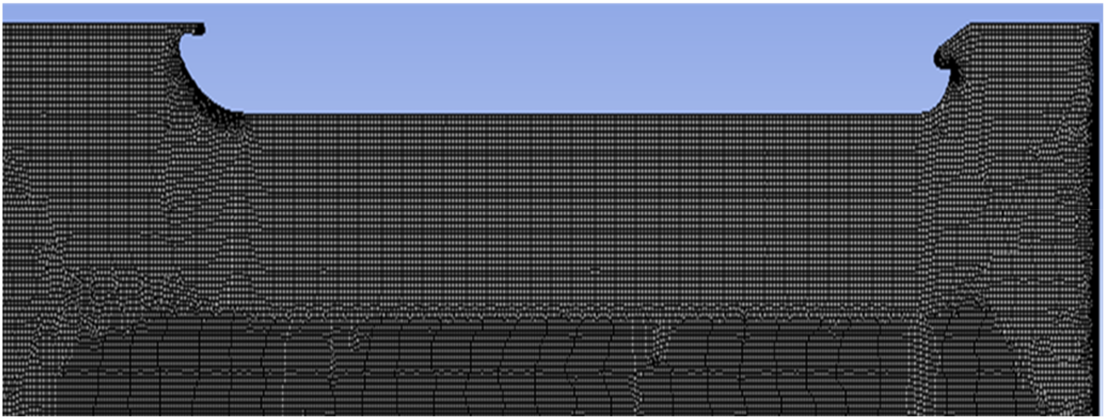
Figure 2.
Meshed air lubrication geometry.

Figure 3.
Distribution of dynamic pressure in the flow-field.
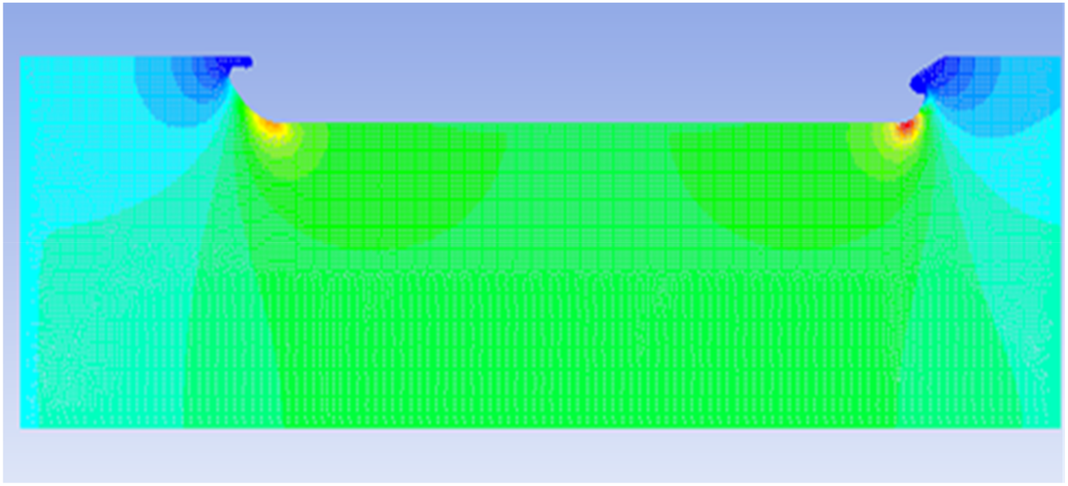
Figure 4.
Skin friction coefficient on the non-air lubricated hull.

Figure 5.
Distribution of dynamic pressure in the flow-field with air lubrication.

Figure 6.
Skin friction coefficient on the air lubricated hull.
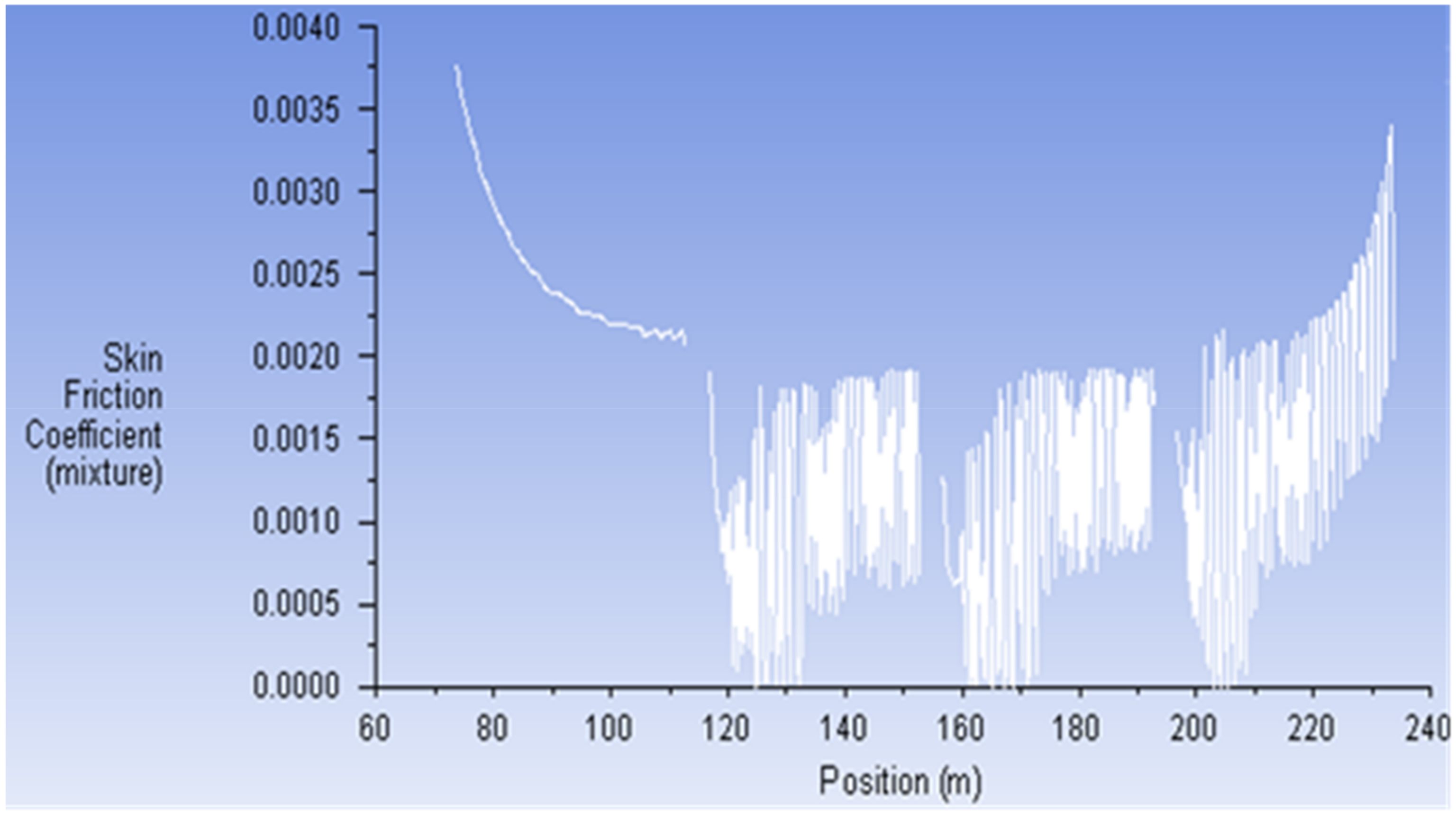
Figure 7.
Snapshot from the operation of air lubrication system.

Figure 8.
Virtualization of the flow Seawater and Bubbles.

Figure 9.
Main Wartsila propulsive engine.

Figure 10.
Representation of an integrated system in a ship.
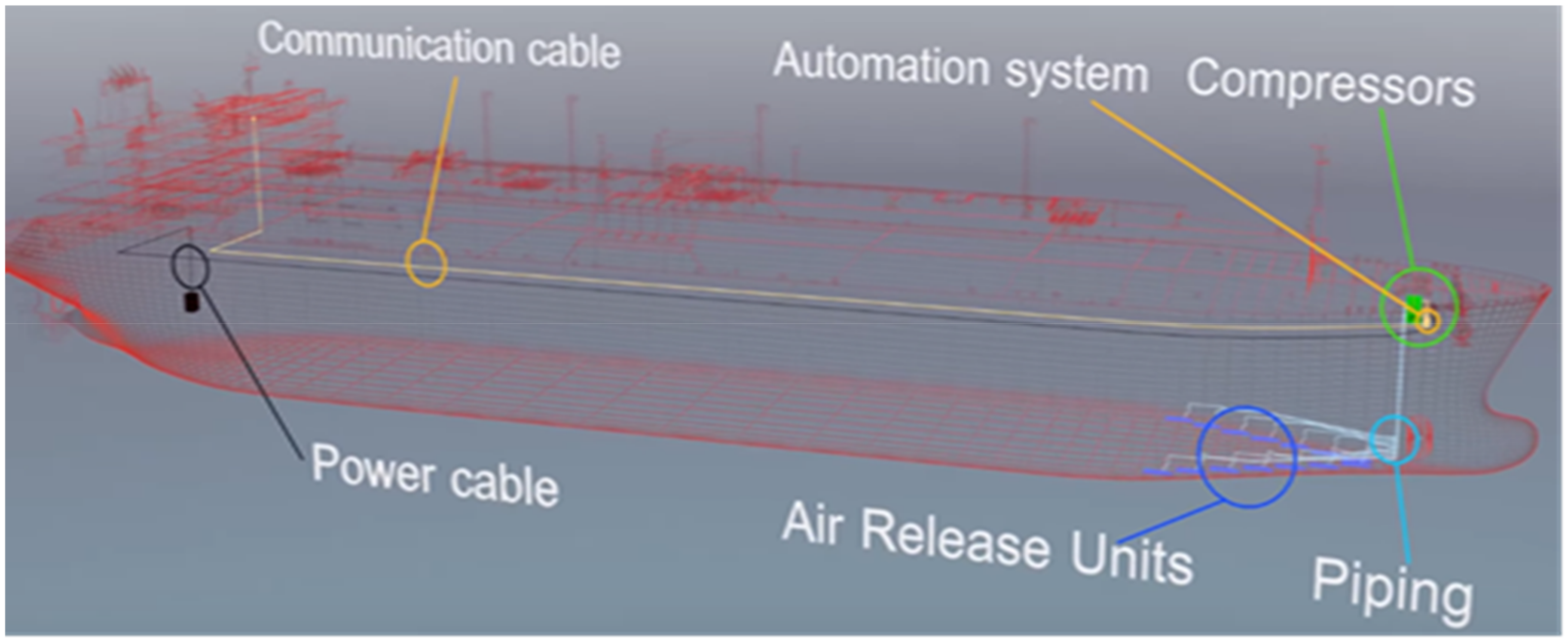
Figure 11.
(a) Ingersoll Rand Suitable compressor; (b) Piping system.

Figure 12.
Silverstream Technologies’ arrow-formation of injectors.
Figure 13.
Mitsubishi Heavy Industries’ double curtain-formation of injectors.


Table 1.
Explanation of main abbreviations.
| CT | Total Resistance Coefficient |
|---|---|
| Cf | Hull’s skin friction coefficient |
| CA | Increase in resistance due to the ship’s volume |
| CAA | Air resistance coefficient |
| CR | Residual resistance coefficient |
| SFC | Specific Fuel Consumption of engine |
| FT | Total propulsive resistance |
| P | Propulsive power |
| FC | Fuel consumption |
| M | Amount of money spent |
| E | Amount of CO2 emissions calculated |
© 2020 by the authors. Licensee MDPI, Basel, Switzerland. This article is an open access article distributed under the terms and conditions of the Creative Commons Attribution (CC BY) license (http://creativecommons.org/licenses/by/4.0/).
Share and Cite
MDPI and ACS Style
Fotopoulos, A.G.; Margaris, D.P. Computational Analysis of Air Lubrication System for Commercial Shipping and Impacts on Fuel Consumption. Computation 2020, 8, 38. https://0-doi-org.brum.beds.ac.uk/10.3390/computation8020038
AMA Style
Fotopoulos AG, Margaris DP. Computational Analysis of Air Lubrication System for Commercial Shipping and Impacts on Fuel Consumption. Computation. 2020; 8(2):38. https://0-doi-org.brum.beds.ac.uk/10.3390/computation8020038
Chicago/Turabian StyleFotopoulos, Andreas G., and Dionissios P. Margaris. 2020. "Computational Analysis of Air Lubrication System for Commercial Shipping and Impacts on Fuel Consumption" Computation 8, no. 2: 38. https://0-doi-org.brum.beds.ac.uk/10.3390/computation8020038
Note that from the first issue of 2016, this journal uses article numbers instead of page numbers. See further details here.