Evaluation of a Near-Wall-Modeled Large Eddy Lattice Boltzmann Method for the Analysis of Complex Flows Relevant to IC Engines

Abstract

In this paper, we compare the capabilities of two open source near-wall-modeled large eddy simulation (NWM-LES) approaches regarding prediction accuracy, computational costs and ease of use to predict complex turbulent flows relevant to internal combustion (IC) engines. The applied open source tools are the commonly used OpenFOAM, based on the finite volume method (FVM), and OpenLB, an implementation of the lattice Boltzmann method (LBM). The near-wall region is modeled by the Musker equation coupled to a van Driest damped Smagorinsky-Lilly sub-grid scale model to decrease the required mesh resolution. The results of both frameworks are compared to a stationary engine flow bench experiment by means of particle image velocimetry (PIV). The validation covers a detailed error analysis using time-averaged and root mean square (RMS) velocity fields. Grid studies are performed to examine the performance of the two solvers. In addition, the differences in the processes of grid generation are highlighted. The performance results show that the OpenLB approach is on average 32 times faster than the OpenFOAM implementation for the tested configurations. This indicates the potential of LBM for the simulation of IC engine-relevant complex turbulent flows using NWM-LES with computationally economic costs.

1. Introduction

Due to the complex turbulent nature of internal combustion (IC) engine flows, their accurate prediction is a major challenge to numerical and experimental investigations. Additional difficulties arise from the interconnection of multiphysical processes, including multiphase flow phenomena, heat transfer and chemical reactions. Each process features different time and length scales, often varying in orders of magnitude, which further increases the complexity.

A particularly important turbulent flow structure for the analysis of IC engines is the intake jet [1]. This high-speed flow over the valves is critical in generating a charge motion, which is commonly referred to as a tumble motion. The tumble breakdown in engine compression results in turbulent structures, which dominate the mixing, ignition and combustion processes and in turn, the engine efficiency and pollutant emissions. Therefore, it is necessary to understand the complex processes in turbulent IC engine intake flows to improve the combustion performance and reduce cycle-to-cycle variability [2,3,4,5,6,7].

Optically accessible research engines enable the detailed investigation and visualization of the processes inside IC engines, often with simplified geometries for numerical validation. High-speed laser diagnostics have long been utilized in engine experiments and have provided more insight into the turbulent structures present in engine flows [8,9,10,11]. Simplified flow bench setups with steady state or transient operation are common tools to optimize cylinder head or intake port geometries and have been used to investigate the intake flow in industrial and scientific research [12,13]. Recent studies examined intake phenomena using magnetic resonance velocimetry (MRV) in a steady water flow bench [1] or low-speed particle image velocimetry (PIV) in a steady air flow bench [14,15]. The data from these experiments have been used as validation for large eddy simulation (LES) approaches [14,15,16,17,18].

However, high-speed PIV data for a flow bench with a realistic engine geometry is limited. Therefore, numerical simulations are another essential tool for the analysis of IC engine flows. In particular, the 3D flow data and turbulence structures obtained with LES offer data which are nearly impossible to obtain in experimental investigations. The choice of LES instead of commonly used Reynolds-averaged Navier–Stokes (RANS) approaches is justified by its ability to resolve the intrinsic unsteady flow motion resulting from the moving valves and pistons. The study of unsteady phenomena such as cycle-to-cycle variability, misfire and knock are especially important factors influencing the geometric design and the operating conditions [2]. The use of LES, which is known to be computationally expensive, is often favored with moderate Reynolds numbers ($10,000<\mathrm{Re}<30,000$) and relatively small regions of interest. However, the fast prediction of accurate and detailed LES results to accelerate design cycles is still a challenge due to the increased number of cells and time required to generate adequate statistics when comparison with RANS approaches.

LES studies of fired and non-fired engine cases including moving piston and valves are reported by many researchers, e.g., [3,4,5,6,7]. Most of these numerical studies are focused on the analysis of cycle-to-cycle variations of in-cylinder flow fields and its influence on the mixing dynamics, combustion and pollutant emission. In this respect, it is worth mentioning that systematic evaluation studies of different LES approaches and models under engine-like operating conditions are rarely reported in the literature. This is mainly because of the considerable numerical effort required to carry out LES of many engine cycles of fired and non-fired cases with moving piston/valves. Furthermore, the complexity of in-cylinder flows impedes in-depth studies of individual processes and model evaluation. Therefore, it is useful to reduce the complexity of the engine configuration and evaluate LES approaches and numerical models by means of simplified flow bench configurations that represent most of the flow and mixing phenomena relevant to IC engines.

The aforementioned studies are based on traditional discretization methods like the finite volume method (FVM). In recent years, an alternative approach called the lattice Boltzmann method (LBM) has gained increasing attention in research and industry. LBM is useful in a wide range of applications, e.g., thermal flow simulations [19,20] or flows in complex geometries [21,22], due to its highly efficient parallel algorithm [23,24]. Such efficiency offers a high potential in reducing computation times for the simulation of high Reynolds number flows using DNS or LES approaches, which is usually a bottleneck in the field of turbulent flow simulations.

Qualitative and quantitative comparisons were made to estimate the capabilities of LBM based implementations for the simulation of turbulent flows in comparison with FVM-based implementations. In 2014 Kajzer et al. [25] evaluated the performance differences between an LBM and FVM implementation for the simulation of homogeneous isotropic turbulence. They found that in particular the scalability of LBM methods and the adaptivity for computations on graphics processing units (GPU) lead to a significant performance advantage compared with the tested FVM implementation in OpenFOAM. Two years later Pasquali et al. [26] showed that the calculation of the external aerodynamics of a car also benefits from the use of LBM on GPUs. A further comparison between LBM and FVM depicted that the higher grid resolution obtained by LBM leads to more resolved vortex structures in the outer layer of turbulent channel flows [27]. Barad et al. [28] compared a higher order finite difference method (FDM) with LBM in a software framework that uses the same Cartesian mesh structure. They showed that for the simulation of airframe noise the LBM implementation is 15 times faster than the higher order FDM scheme at a similar accuracy.

Most of the LBM studies related to engine flows that have been conducted to date deal with the injection process. Therefore, a multiphase approach is chosen to simulate spray formation, bubble break up and flow induced cavitation. A summary of these studies can be found in the book of Montessori and Falcucci [29]. A moving valve/pistion arrangement was simulated by Dorschner et al. [30] using the parameter-free Karlin–Bösch–Chikatamarla (KBC) collision operator. They showed that the results are in good agreement with a DNS reference.

In contrast to all these previous contributions, we focus on the implementation of open source near-wall-modeled LES (NWM-LES) to achieve fast and accurate results, which is relevant to users in academia and industry. Therefore, a recent version of the established FVM-based implementation of OpenFOAM is compared with OpenLB [31], an open source LBM framework. To get a fair comparison, we solve the same target equation in both software frameworks, including an explicit sub-grid scale (SGS) modeling and the use of a wall function. Furthermore, we do not limit the grid to a certain amount of cells or type of mesh elements so that each implementation can show its advantages. The grid generation process is also taken into account to compare the time spent on pre-processing. This is one of the first studies where in-house-conducted experimental data are used to validate two open source implementations. Moreover, a detailed error analysis of both methods covering the grid convergence of time-averaged and root mean square (RMS) velocity fields in the context of engine flows is a novelty. Additionally, a performance analysis compares the solver runtime of each implementation that is needed to calculate the statistics for the different grids. The comparison in the theory section aims to highlight the differences between both discretization methods. In addition, the differences in the implementation of wall-modeled LES in LBM and FVM are described. The NWM-LES implementation in LBM is ongoing research due to the complex boundary treatment in LBM. As a result, a new LBM wall function approach is proposed which extends the previous approaches [32,33] to curved boundaries.

This paper is organized as follows: Section 2 introduces the applied modeling approaches and shows the differences and similarities using LBM or FVM. Next, the experimental and numerical setup is described in Section 3. The related results using NWM-LES obtained with OpenFOAM and OpenLB for different grid resolutions are presented and compared to the PIV results in Section 4. Finally, Section 5 summarizes the results and draws a conclusion.

2. Applied Modeling Approaches

2.1. Filtered Navier–Stokes Equations

The filtered incompressible Navier–Stokes equations consist of the continuity equation

$$\frac{\partial {\overline{u}}_{\alpha }}{\partial x_{\alpha }}=0,$$

(1)

and the momentum equation according Leonard’s decomposition [34] which reads

$$\frac{\partial {\overline{u}}_{\alpha }}{\partial t}+\frac{\partial {\overline{u}}_{\alpha }{\overline{u}}_{\beta }}{\partial x_{\beta }}=\nu \frac{\partial }{\partial x_{\beta }}\left(\frac{\partial {\overline{u}}_{\alpha }}{\partial x_{\beta }}+\frac{\partial {\overline{u}}_{\beta }}{\partial x_{\alpha }}\right)-\frac{\partial T_{\alpha \beta }^{\mathrm{SGS}}}{\partial x_{\beta }}-\frac{1}{\rho }\frac{\partial \overline{p}}{x_{\alpha }},$$

(2)

where Greek indices obey the Einstein notation, ${\overline{u}}_{\alpha }$ is the filtered velocity, $\overline{p}$ is the filtered pressure field, $T_{\alpha \beta }^{\mathrm{SGS}}$ is the SGS stress tensor, $\rho$ is the density and $\nu$ is the viscosity. This set of equations can be closed by using a linear eddy viscosity hypothesis for the SGS stress tensor

$$T_{\alpha \beta }^{\mathrm{SGS}}=-{\nu }^{\mathrm{SGS}}\left(\frac{\partial {\overline{u}}_{\alpha }}{\partial x_{\beta }}+\frac{\partial {\overline{u}}_{\beta }}{\partial x_{\alpha }}\right),$$

(3)

where ${\nu }^{\mathrm{SGS}}$ is the SGS viscosity that can be modeled by an SGS viscosity model (see Section 2.2). In Equation (2) no volume force is applied and will not be considered hereafter.

2.1.1. Finite Volume Method

In dealing with the FVM of incompressible fluid flow, the discretization process of the balance laws of fluid motion can be divided into two steps: (1) the spatial and temporal discretization of the solution domain and (2) the discretization of the spatial and temporal terms in the Navier–Stokes equations [35]. Then, the partial differential equations can be converted into a corresponding set of algebraic equations and solved numerically. Additionally, nonlinearities in the Navier–Stokes equations and the pressure-velocity coupling require some special numerical treatment. The second-order solution procedure employed in the open source C++ library OpenFOAM 2.4.0, which is used in the present LES study, is briefly outlined in the following. A detailed description can be found, e.g., in [36,37,38].

In the standard FVM framework of OpenFOAM, the continuum space and time domain are divided into a finite number of discrete regions called control volumes (CV) and time intervals, respectively. Thereby, the CVs completely bound the solution domain and the solution variables, such as velocity and pressure, are colocated at the cell centroids of the CVs [39]. In contrast to a staggered grid arrangement, this allows an arbitrary topology of CVs, e.g., hexahedrons, tetrahedrons, prisms, pyramids or general polyhedrons, which has significant advantages in the discretization of complex solution domains.

Several approximation schemes and solution procedures are available in the OpenFOAM framework to discretize and solve the Navier-Stokes equations. In this study, the standard pimpleFOAM solver of OpenFOAM 2.4.0 is applied, which is based on a merged PISO [40]-SIMPLE [41] algorithm for the coupling of pressure and velocity. Thereby, the governing equations are numerically solved in a segregated manner using a momentum predictor, pressure solver and momentum corrector. This iterative solution procedure is applied with a second-order implicit backward-differencing scheme for the time integration. Regarding spatial terms, a low-dissipative second-order flux-limiting differencing scheme is employed for the convection terms and a conservative scheme is used for the Laplacian and gradient terms. The resulting systems of linear equations are iteratively solved using a geometric agglomerated algebraic multigrid solver. Thereby, convergence of the overall procedure is obtained if all normalized residuals are smaller than ${10}^{-4}$. Validation and verification studies of this specific solution procedure for LES of complex fluid flows relevant to IC engines are provided in [18,42,43].

2.1.2. Lattice Boltzmann Method

The lattice Boltzmann equation discretizes the velocity space of the kinetic Boltzmann equation to a discrete set of lattice velocities $c_i$, $i=0,1,\dots ,q-1$. Common velocity sets to recover the three-dimensional incompressible Navier–Stokes equations are $D3Q15$, $D3Q19$ and $D3Q27$. The present work uses a discrete velocity $D3Q19$ set, which is given by

$$c_i=\left\{\begin{array}{cc}(0,0,0)\hfill & i=0\hfill \\ (\pm 1,0,0),(0,\pm 1,0),(0,0,\pm 1)\hfill & i=1,2,\dots ,6\hfill \\ (\pm 1,\pm 1,0),(\pm 1,0,\pm 1),(0,\pm 1,\pm 1)\hfill & i=7,8,\dots ,18\hfill \end{array}\right.$$

(4)

The descriptor set is chosen due to the higher computation performance and the lower memory demand in the used LBM implementation. However, higher errors due to a violation of the rotational invariance are taken into account in comparison with a $D3Q27$ stencil [44].

The filtered lattice Boltzmann equation without external forces is given by

$${\overline{f}}_i\left(x^{\mathrm{LB}}+c_i,t^{\mathrm{LB}}+1\right)={\overline{f}}_i\left(x^{\mathrm{LB}},t^{\mathrm{LB}}\right)+{\overline{\mathsf{\Omega }}}_i,$$

(5)

where ${\overline{f}}_i$ is the filtered particle distribution function at discrete lattice position $x^{\mathrm{LB}}$ and time step $t^{\mathrm{LB}}$. The filtered collision operator ${\overline{\mathsf{\Omega }}}_i$ is implemented by a single-relaxation time model proposed by Bhatnagar, Gross and Krook [45]. It can be written as

$${\overline{\mathsf{\Omega }}}_i=-\frac{1}{{\tau }^{eff}}\left({\overline{f}}_i(t^{\mathrm{LB}},x^{\mathrm{LB}})-{\overline{f}}_i^{eq}({\overline{\rho }}^{\mathrm{LB}},{\overline{u}}^{\mathrm{LB}})\right),$$

(6)

where ${\tau }^{eff}$ is the effective relaxation time towards the filtered discrete particle distribution function at equilibrium state ${\overline{f}}_i^{eq}$, $\overline{\rho }$ is the filtered lattice density and $\overline{u}$ the filtered velocity field. The collision operator satisfies the conservation of mass and momentum. The particle distribution function equilibrium is described by a low Mach number truncated Maxwell-Boltzmann distribution

$${\overline{f}}_i^{eq}\left({\overline{\rho }}^{\mathrm{LB}},{\overline{u}}^{\mathrm{LB}}\right)={\overline{\rho }}^{\mathrm{LB}}{\omega }_i\left[1+\frac{c_{i\alpha }{\overline{u}}_{\alpha }^{\mathrm{LB}}}{c_s^2}+\frac{{\overline{u}}_{\alpha }^{\mathrm{LB}}{\overline{u}}_{\beta }^{\mathrm{LB}}(c_{i\alpha }{c}_{i\beta }-c_s^2{\delta }_{\alpha \beta })}{2c_s^4}\right],$$

(7)

where ${\omega }_i$ are the lattice weights obtained by the Gauss-Hermite quadrature [46,47], $c_s=1/\sqrt{3}$ is the speed of sound of the lattice and ${\delta }_{\alpha \beta }$ is the Kronecker operator.

The moments of the particle distribution functions ${\overline{f}}_i$ yield macroscopic flow quantities. The density ${\overline{\rho }}^{\mathrm{LB}}$, the momentum ${\overline{\rho }}^{\mathrm{LB}}{\overline{u}}^{\mathrm{LB}}$ and momentum flux $\overline{\mathsf{\Pi }}$ are obtained by the zeroth, first and second moments, which are given by

$${\overline{\rho }}^{\mathrm{LB}}=\sum _{i=0}^{q-1}{\overline{f}}_i,$$

(8)

$${\overline{\rho }}^{\mathrm{LB}}{\overline{u}}^{\mathrm{LB}}=\sum _{i=0}^{q-1}{c}_i{\overline{f}}_i,$$

(9)

$${\overline{\mathsf{\Pi }}}_{\alpha \beta }=\sum _{i=0}^{q-1}{c}_{i\alpha }{c}_{i\beta }{\overline{f}}_i.$$

(10)

The lattice effective kinematic viscosity of the fluid ${\nu }^{eff}$ is connected to the effective relaxation time ${\tau }^{eff}$ as follows

$${\nu }^{\mathrm{LB},eff}=c_s^2\left({\tau }^{eff}-0.5\right).$$

(11)

Assuming a simplified isothermal equation of state the filtered lattice pressure is related to the filtered density by

$${\overline{p}}^{\mathrm{LB}}=c_s^2{\overline{\rho }}^{\mathrm{LB}}.$$

(12)

Finally, the lattice Boltzmann algorithm is divided in 2 steps: the collision step and the streaming step. The local collision step is represented by the right-hand side of Equation (5) and the subsequent streaming step is associated with the left-hand side of Equation (5).

2.2. Sub-Grid Scale Modeling

The introduced eddy viscosity ${\nu }^{\mathrm{SGS}}$ in Equation (3) is estimated by an SGS viscosity model, which can be generally written as

$${\nu }^{\mathrm{SGS}}={\left(C_M{\Delta }_{grid}\right)}^2{D}_M,$$

(13)

where $C_M$ is a model coefficient, ${\Delta }_{grid}$ is the grid filter and $D_M$ a model-related operator. The present work uses a Smagorinsky-Lilly model [48], where the model operator is defined as

$$D_M=\sqrt{2{\overline{S}}_{\alpha \beta }{\overline{S}}_{\alpha \beta }},$$

(14)

where ${\overline{S}}_{\alpha \beta }$ is the filtered strain rate. The literature values for the Smagorinsky-Lilly model constant $C_M$ are in the range of $C_M=0.065\dots 0.24$ [49,50]. For a complex turbulent flow, a Smagorinsky-Lilly constant of $C_M=0.1$ is a common choice [51]. The Smagorinsky–Lilly model suffers from a too dissipative behavior in the near-wall region [42,52]. One possibility to prevent this aspect is the introduction of a damping function that reduces the SGS viscosity depending on the wall distance. The van Driest damping function [53] can be incorporated in the grid filter ${\Delta }_{grid}$ by

$${\Delta }_{grid}=min\left[\sqrt[3]{{\Delta }_x{\Delta }_y{\Delta }_z},\frac{\kappa y}{C_{\Delta }}\left(1-e^{(-\frac{y^{+}}{A^{+}})}\right)\right],$$

(15)

where y is the wall distance, $A^{+}=26$ is the van Driest parameter, $C_{\Delta }=0.158$ is a model constant and $\kappa =0.41$ is the von Kármán constant [54]. The dimensionless wall distance $y^{+}$ in Equation (15) is defined as

$$y^{+}=\frac{u_{\tau }y}{\nu },$$

(16)

where $u_{\tau }=\sqrt{\frac{T_w}{\rho }}$ is the friction velocity and $T_w$ the wall shear stress.

2.2.1. SGS Model for Finite Volume Method

In the FVM framework of OpenFOAM, the SGS viscosity ${\nu }^{\mathrm{SGS}}$ is calculated explicitly for each time step using the resolved velocity field. Then, the turbulent and molecular diffusion contributions are combined into an effective stress tensor by means of the Boussinesq approximation as

$$\begin{array}{cc}\hfill T_{\alpha \beta }^{eff}& =-\left(\nu +{\nu }^{\mathrm{SGS}}\right)\left(\frac{\partial {\overline{u}}_{\alpha }}{\partial x_{\beta }}+\frac{\partial {\overline{u}}_{\beta }}{\partial x_{\alpha }}\right),\hfill \\ \hfill & =-{\nu }^{eff}\left(\frac{\partial {\overline{u}}_{\alpha }}{\partial x_{\beta }}+\frac{\partial {\overline{u}}_{\beta }}{\partial x_{\alpha }}\right),\hfill \end{array}$$

(17)

where ${\nu }^{eff}$ represents the effective viscosity. For the sake of computational efficiency, the velocity gradient and transposed velocity gradient terms in Equation (17) are treated separately. Thereby, the velocity gradient term is treated implicitly as a diffusion, while the transposed velocity is treated as an explicit source term. The latter is therefore calculated using the velocity at the previous iteration. Further information on the implementation of eddy viscosity turbulence in OpenFOAM can be found, e.g., in [55].

2.2.2. SGS Model for Lattice Boltzmann Method

Eddy viscosity models are often introduced in LBM by adding turbulent viscosity to the molecular viscosity [56], which results in an effective viscosity

$${\nu }^{\mathrm{LB},eff}={\nu }^{\mathrm{LB}}+{\nu }^{\mathrm{LB},\mathrm{SGS}}.$$

(18)

A consistent approach to implement eddy viscosity models in LBM was derived by Malaspinas and Sagaut [57]. They presented that due to the connection between lattice viscosity and lattice relaxation time (see Equation (11)), the relaxation time is also divided in a molecular and SGS contribution

$${\tau }^{eff}=\tau +{\tau }^{\mathrm{SGS}},$$

(19)

where ${\tau }^{\mathrm{SGS}}=\frac{{\nu }^{\mathrm{LB},\mathrm{SGS}}}{c_s^2}$ is the eddy contribution. The filtered strain rate ${\overline{S}}_{\alpha \beta }^{\mathrm{LB}}$ in the SGS operator formulation in Equation (14) can be obtained by a finite difference scheme or locally in the LBM framework by

$${\overline{S}}_{\alpha \beta }^{\mathrm{LB}}=-\frac{{\overline{\mathsf{\Pi }}}_{\alpha \beta }^{neq}}{2{\overline{\rho }}^{\mathrm{LB}}{\tau }^{eff}{c}_s^2},$$

(20)

where ${\overline{\mathsf{\Pi }}}_{\alpha \beta }^{neq}$ is the second moment of the non-equilibrium parts of the particle distribution function, which can be calculated according to Equation (10) by replacing ${\overline{f}}_i$ with ${\overline{f}}_i^{neq}=({\overline{f}}_i-{\overline{f}}_i^{eq})$. This implicit relation of the effective relaxation time ${\tau }^{eff}$ and the filtered strain rate ${\overline{S}}_{\alpha \beta }^{\mathrm{LB}}$ can be replaced by an explicit expression for the Bhatnagar–Gross–Krook (BGK) collision operator by a local method proposed by Malaspinas and Sagaut [57]. This explicit expression for determining the effective relaxation time ${\tau }^{eff}$ is given by

$${\tau }^{eff}=\sqrt{{\tau }^2+\frac{2C_M^2}{{\overline{\rho }}^{\mathrm{LB}}{c}_s^4}\sqrt{2{\overline{\mathsf{\Pi }}}_{\alpha \beta }^{neq}{\overline{\mathsf{\Pi }}}_{\alpha \beta }^{neq}}}+\frac{\tau }{2}.$$

(21)

2.3. Wall Function Approach

In contrast to a near-wall resolved LES, the NWM-LES requires additional effort to model the effects occurring in the boundary layer. However, NWM-LES allows grid spacing up to $y^{+}=200$, which results in a significantly smaller amount of grid points. In the present work, we use the idea of Werner and Wengle [58], which describes an instantaneous connection between the wall shear stress and the velocity. This consideration only applies for averaged quantities and therefore a RANS hypothesis is assumed for the boundary node. A fully developed turbulent boundary layer can be described by the Musker profile [59] which reads

$$\begin{array}{cc}\hfill u^{+}& =5.424arctan\left(\frac{2.0y^{+}-8.15}{16.7}\right)\hfill \\ \hfill & +{log}_{10}\left(\frac{{(y^{+}+10.6)}^{9.6}}{{(y^{{+}^2}-8.15y^{+}+86.0)}^2}\right)\hfill \\ \hfill & -3.5072790194.\hfill \end{array}$$

(22)

This empirical formulation is based on a logarithmic law and is able to describe the turbulent boundary layer from the viscous sublayer ($y^{+}\ge 1$). The solution of the implicit function (22) requires an iterative scheme.

2.3.1. Wall Function for Finite Volume Method

Analogous to wall-shear stress models often used in the context of RANS, the boundary condition of the SGS viscosity ${\nu }^{\mathrm{SGS}}$ is corrected for each time step by means of a wall function in the NWM-LES approach of OpenFOAM. The numerical procedure can be divided into two steps. First, the friction velocity $u_{\tau }$ is approximated iteratively according to Musker’s wall function. Thereby, the Newton–Raphson method is applied to find the root of the wall function. Then, in the second step, ${\nu }^{\mathrm{SGS}}$ at the wall is calculated as

$${\nu }^{\mathrm{SGS}}=u_{\tau }^2\frac{y_p}{u_{\Vert }},$$

(23)

where $y_p$ denotes the wall distance of the cell centroid and $u_{\Vert }$ the stream-wise velocity. It is important to note that a boundary condition of ${\nu }^{\mathrm{SGS}}$ based on Musker’s wall function is not available in OpenFOAM and was therefore added to the standard framework. A detailed description of the wall function approach in OpenFOAM including comprehensive validation studies in turbulent channel and impinging flows were provided by the authors in [60].

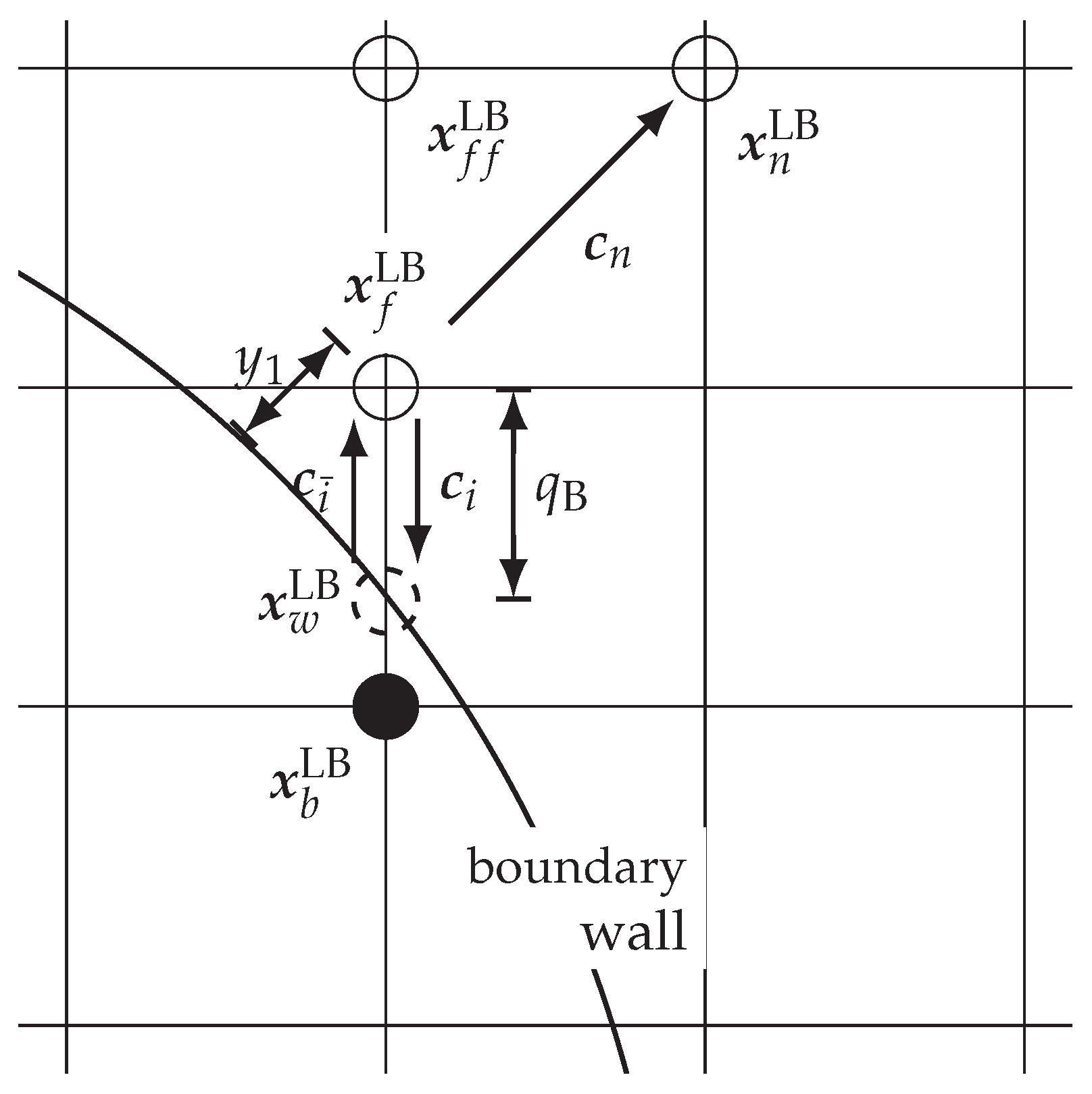
2.3.2. Wall Function for Lattice Boltzmann Method

The implementation of wall functions in the context of LBM is not straightforward due to numerous boundary scheme approaches. The idea of the wall model approach applied in this work was proposed by Malaspinas and Sagaut [32] and adapted to the BGK collision operator by Haussmann et al. [33]. They validated the wall function scheme using a bi-periodic turbulent channel flow. We adapt this scheme to curved boundaries using a curved link-wise instead of a wet-node boundary scheme. Our proposed algorithm is parted in two steps: the curved boundary approach and a velocity correction step according to the wall function. For better comprehension, the used indexing convention for the following two paragraphs is depicted in Figure 1.

Curved Boundary Step

In the present work, we use the curved boundary approach proposed by Bouzidi et al. [61]. This approach is an extension of a half-way bounce back scheme and characterized as precise, stable and computationally efficient for the simulation of turbulent flows [62]. The interpolated bounce-back approach uses a linear interpolation based on the dimensionless distance $q_{\mathrm{B}}$, which is defined as:

$$q_{\mathrm{B}}=\frac{|x_f^{\mathrm{LB}}-x_w^{\mathrm{LB}}|}{|x_f^{\mathrm{LB}}-x_b^{\mathrm{LB}}|}.$$

(24)

Without altering the streaming step for boundary cells the unknown particle distribution function after the streaming step $f_{\overline{i}}(x_f^{\mathrm{LB}},t^{\mathrm{LB}}+1)$ can be replaced by

$$f_{\overline{i}}(x_f^{\mathrm{LB}},t^{\mathrm{LB}}+1)=\left\{\begin{array}{cc}\frac{1}{2q_{\mathrm{B}}}{f}_i(x_b^{\mathrm{LB}},t^{\mathrm{LB}}+1)+\frac{2q_{\mathrm{B}}-1}{2q_{\mathrm{B}}}{f}_{\overline{i}}(x_{ff}^{\mathrm{LB}},t^{\mathrm{LB}}+1)\hfill & \mathrm{for}{q}_{\mathrm{B}}\ge \frac{1}{2},\hfill \\ 2q_{\mathrm{B}}{f}_i(x_b^{\mathrm{LB}},t^{\mathrm{LB}}+1)+(1-2q_{\mathrm{B}})f_i(x_f^{\mathrm{LB}},t^{\mathrm{LB}}+1)\hfill & \mathrm{for}{q}_{\mathrm{B}}<\frac{1}{2},\hfill \end{array}\right.$$

(25)

where index $\overline{i}$ indicates the particle distribution function in the opposite direction of index i. For $q_{\mathrm{B}}=0.5$ the approach is equal to the half-way bounce back boundary condition.

Velocity Correction Step

The velocity correction step is used to correct the velocity in the particle distribution functions at node position $x_f^{\mathrm{LB}}$ according the wall function. Firstly, the distance to the boundary $y_1^{\mathrm{LB}}$ is defined in the discrete normal direction $c_n$. Accordingly, the distance from the neighbor fluid node at position $x_n^{\mathrm{LB}}$ to the boundary is given by

$$y_2^{\mathrm{LB}}=y_1^{\mathrm{LB}}+\left|c_n\right|.$$

(26)

Due to the fact that the wall profile uses only the stream-wise velocity component, a local stream-wise unit vector ${\mathbf{e}}_s$ is obtained by

$${\mathbf{e}}_s=\frac{{\overline{u}}_n^{\mathrm{LB}}-({\overline{u}}_n^{\mathrm{LB}}·c_n)c_n}{|{\overline{u}}_n^{\mathrm{LB}}-({\overline{u}}_n^{\mathrm{LB}}·c_n)c_n|}.$$

(27)

Subsequently, the stream-wise component ${\overline{u}}_2^{\mathrm{LB}}$ of ${\overline{\mathbf{u}}}_n^{\mathrm{LB}}$ is calculated by

$${\overline{u}}_2^{\mathrm{LB}}={\overline{u}}_n^{\mathrm{LB}}·{\mathbf{e}}_s.$$

(28)

The boundary distance $y_2^{\mathrm{LB}}$ and the stream-wise velocity component ${\overline{u}}_2^{\mathrm{LB}}$ are inserted in the Musker profile Equation (22) to obtain the averaged wall shear stress ${\tilde{T}}_w^{\mathrm{LB}}$. Therefore, the solution of the implicit equation is approximated by the Newton method. Afterwards, the stream-wise component ${\tilde{u}}_1^{\mathrm{LB}}$ of ${\tilde{u}}_f^{\mathrm{LB}}$ is calculated by the Musker profile Equation (22) using the boundary distance $y_1^{\mathrm{LB}}$ and the averaged wall shear stress ${\tilde{T}}_w^{\mathrm{LB}}$. Then, the velocity ${\tilde{u}}_f^{\mathrm{LB}}$ of the first fluid is computed by

$${\tilde{u}}_1^{\mathrm{LB}}={\tilde{u}}_f^{\mathrm{LB}}·{\mathbf{e}}_s.$$

(29)

Finally, the particle distribution function at node position $x_f^{\mathrm{LB}}$ is corrected as follows

$$f_i(x_f^{\mathrm{LB}},t^{\mathrm{LB}}+1)=f_i^{eq}({\rho }^{\mathrm{LB},*},{\tilde{u}}_f^{\mathrm{LB}})+f_i^{neq,*},$$

(30)

where superscript ∗ denotes the quantities calculated after Equation (25). This means only the velocity is altered according the wall function, while the density and the non-equilibrium parts are preserved.

3. Setup of the IC Engine Test Case

In this work, a flow bench setup of an IC engine was chosen as a benchmark for the numerical comparison. With this setup, the intake flow with the focus on the intake jet over the valves into the cylinder can be examined in a realistic engine geometry and at the same time the overall complexity can be reduced compared with a real engine. The optically-accessible single cylinder engine at TU Darmstadt (Darmstadt Engine, 10]) was converted into a steady-state flow bench by removing and replacing the piston with an outlet channel open to ambient conditions (see Figure 2). As opposed to the previous flow bench studies of Freudenhammer et al. [63] in which the same spray-guided cylinder head geometry was fitted in a continuous water flow configuration for MRV measurements, the flow bench of the present study uses dry air and allows for instantaneous flow measurements. For this configuration, the cylinder liner was extended and the outlet channel geometry was optimized by means of unsteady RANS to suppress recirculation of the flow. For added simplicity to the engine geometry, the spark plug and fuel injector were replaced by flat plugs; but otherwise, the four-valve spray-guided pent-roof cylinder head (AVL) and fused-silica cylinder liner with a bore of 86 mm as well as the intake system remained unchanged. Figure 2 shows a diagram of the intake system and engine geometry of the flow bench experiment. As indicated by the red boxes, the flow bench has three optical access sections. The first section (I) represents the standard engine optical access which was fitted to the new flow bench extension (experimental sections II and III). Experimental section II allows for the characterization of the flow inside the flow bench extension for the verification of the flow structures present. Finally, experimental section III allows optical access and flow validation of the outflow through the bottom of the flow bench via a flat fused-silica plate and movable mirror. Intake valves were positioned at a fixed valve lift of 9.21 mm corresponding to 270 °CA (crank angles before top dead center) and exhaust valves were kept closed, thus mimicking the intake flow during regular engine operation.

The flow bench experiment was conducted under controlled boundary conditions for consistent operation. Two mass flow controllers (Bronkhorst) were used to set a defined mass flow of 94.1 $\frac{\mathrm{kg}}{\mathrm{h}}$, which corresponds to the respective instantaneous mass flow at 270 °CA under normal engine operation with a speed of 800 rpm and intake pressure of 0.95 bar. Since the instantaneous mass flow of engine operation is not available, the velocities in the intake jet were compared and matched such that the phase-averaged velocity (average of 400 cycles at 270 °CA) in motored engine operation matched the average velocities of the flow bench near the intake valve. As indicated in Figure 2, two absolute pressure sensors ($P_{in,1}$, $P_{in,2}$, PAA-M8cool HB, Keller) measured the static pressure and two PT100 temperature sensors (${\vartheta }_{in,1}$, ${\vartheta }_{in,2}$) measured the temperature of the flow within the intake pipe. Additionally, two more absolute pressure sensors ($P_{out,1}$, $P_{out,2}$, PMP4070, Kistler) measured the static pressure inside the flow bench.

Table 1. Flow bench boundary conditions. Values in brackets represent estimates of the measurement uncertainty (total error band corresponding to a rectangular distribution with mean ± uncertainty).

Valve Lift	9.21(0.15) mm
${\vartheta }_{in,2}$	22.7(0.5) °C
$P_{in,2}$	1.000(0.001) bar
$P_{out,2}$	0.998(0.001) bar
${\dot{m}}_{in}$	94.10(1.00) kg/hr
$\eta$	$18.26\times {10}^{-6}$ kg/(m s)
$\rho$	1.18 kg/m3
${\vartheta }_{wall}$ (estimated)	22(1) °C

summarizes the experimental boundary conditions.

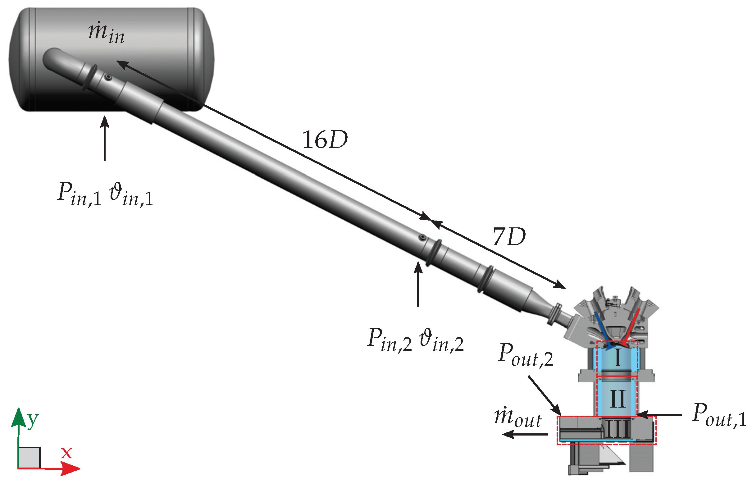
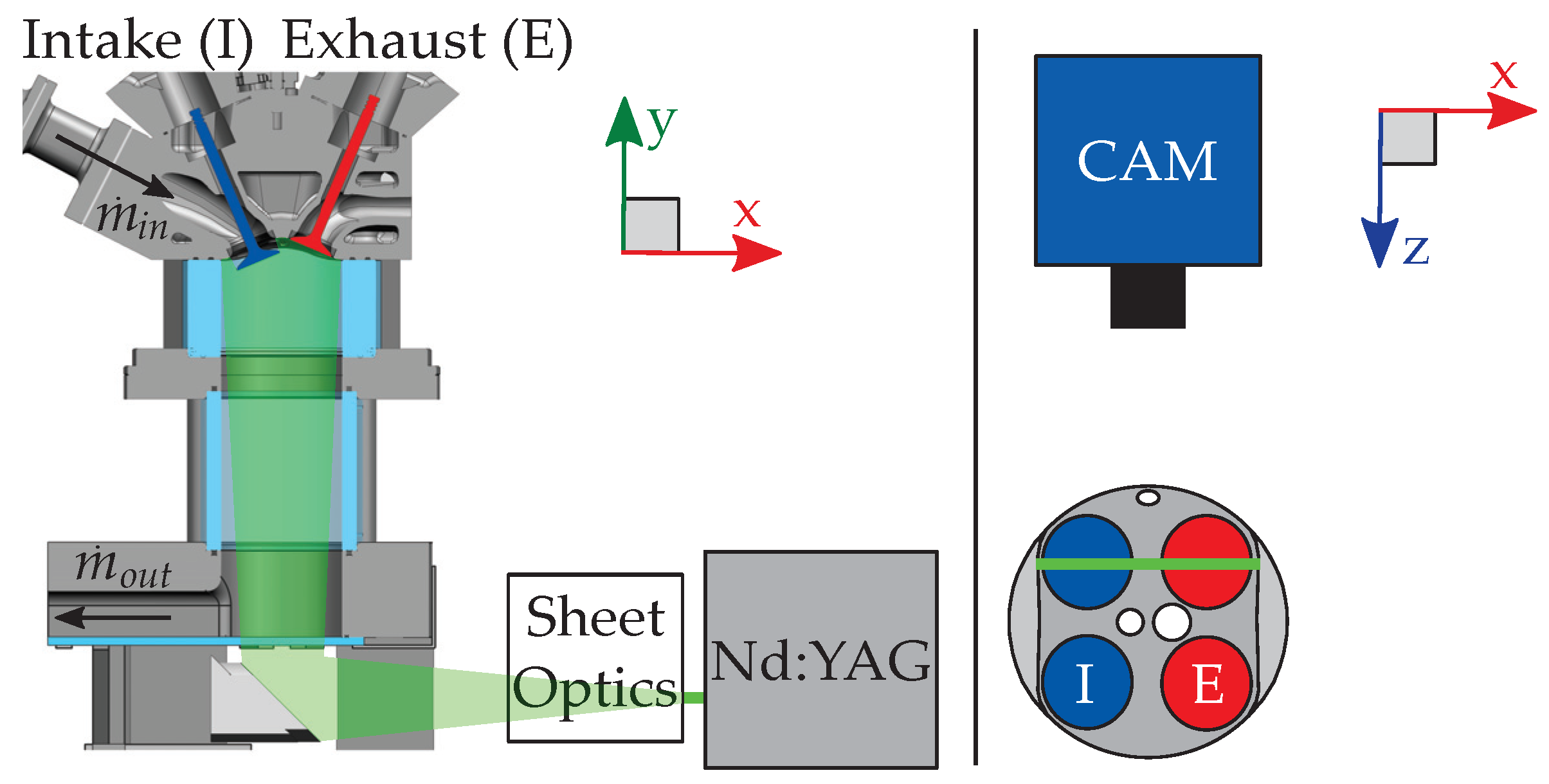
3.1. Experimental Setup

High-speed PIV was used to measure the in-cylinder flow velocity field in the valve plane (VP, z = −19 mm) (see Figure 3). For this configuration a laser light sheet (850 $\mathsf{\mu }$m thickness) from two high-speed frequency-doubled Nd:YAG cavities (IS4II-DE Edgewave), operated at 12.5 kHz each with a time separation of 8 $\mathsf{\mu }$s, entered the cylinder volume via the bottom glass plate of the outlet channel. DOWSIL 510 (Dow Corning) silicone oil was atomized by a fluid seeder (AGF 10.0, Palas) with an average particle size of 0.5 $\mathsf{\mu }$m and introduced to the intake system as tracer particles. The Mie-scattered light was imaged with a high-speed CMOS camera (Phantom v2640) equipped with a Nikon lens (85 mm f/1.4 with 35 mm distance rings) in HS Binned double-frame mode.

The commercial software DaVis 10.0.5 (LaVision) was used to calculate flow fields. After a time filter background subtraction, a cross-correlation with multi-pass iterations of decreasing window size (twice: 48 × 48 pixel; twice: 24 × 24 pixel, 75% overlap) resulted in vector fields which where post-processed with a peak ratio threshold of 1.3 and a universal outlier median filter to remove spurious vectors. The dynamic range of the velocity measurement is limited by the minimum and maximum resolved pixel shift. The frame separation time of the setup was optimized to yield a pixel shift of maximum 4.5 pixels in the intake jet region, since the jet characteristics are the main interest.

The uncertainty of velocity measurements by means of PIV depends on parameters such as the optical setup defined by imaging optics, camera and light sheet as well as tracer properties, the PIV algorithm and the flow itself. Common approaches to estimate the uncertainty as a function of different influencing variables employ artificial PIV images generated by Monte Carlo simulations [64]. Newer methods use the actual experimental data to estimate the uncertainty [65,66,67] and have been validated by a benchmark experiment [68].

The commercial software DaVis estimates the uncertainty based upon a correlation statistics approach [67]. In this study, the time-averaged uncertainty of the instantaneous velocity magnitudes is approximately 3% to 6% (normalized to the global maximum velocity range of 35 m s⁻¹). This uncertainty range is valid for the jet region and lower velocity regions below the valves. Near the exhaust side cylinder walls, where the intake jet is curved downwards due to the influence of the walls, the normalized uncertainties increase to a maximum of 10%. This approach considers random errors inherent to the correlation process for particle images. Therefore, the reported uncertainties apply for instantaneous velocity fields and propagate to RMS velocity values, but are reduced to ≪ 1% for the time-averaged velocity, since most of the 25,000 pairs of particle images are uncorrelated to each other.

Other sources of error introduce a bias in the velocity calculation. Sharp gradients in the flow, e.g., at the edge of the intake jet, are underestimated due to the spatial averaging of the PIV algorithm. Acknowledging reported uncertainty assessments [64], this normalized error is assumed to be on the order of 3% to 9% for the jet region in instantaneous velocity fields and is slightly lower in the time-averaged velocity field due to the non-stationary jet position. The spatial average of the normalized uncertainty due to flow gradients amounts to 1%.

Additional systematic errors stem from the non-zero light sheet thickness and strong out-of-plane velocity components, which are detected as in-plane components due to the camera‘s perspective. This error is zero in the center, increases linearly to the edges of the field-of-view and can amount to more than 10% [64]. However, if the averaged out-of-plane velocity component is zero this error source is statistically zero. In the central tumble plane this assumption is justified, but less so in the valve plane, where mean out-of-plane velocity components exist. The uncertainty due to perspective errors was calculated with the time-averaged LES flow field, which provides all three velocity components. This normalized uncertainty contribution amounts to up to 10% locally and to 0.2% in the spatial average. Altogether, the spatially averaged accumulated normalized uncertainty of the time-averaged PIV measurements within this work is estimated to be 1%.

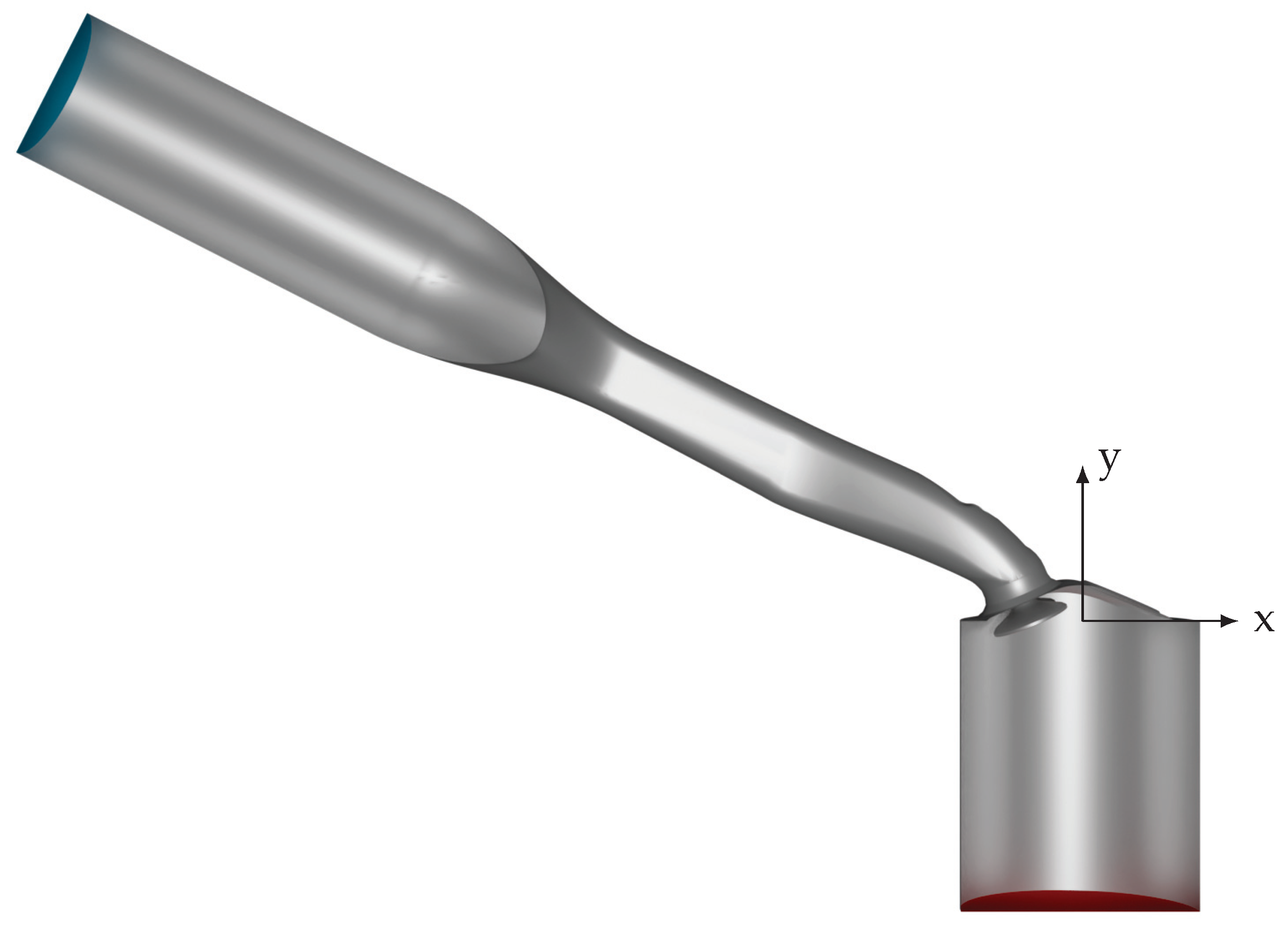
3.2. Numerical Setup

The fluid domain is depicted in Figure 4 in a clip representation. The inlet patch is colored in blue and the outlet patch in red. In contrast to the experimental setup, both the inflow and outflow regions are shortened in order to reduce the computational effort. The reduction of the inflow length to $2.62D$ is justified by the applied inlet boundary condition (see Section 3.3). For the estimation of the outflow length as $1.88D$, the tumble flow area and the integral time scale were considered to ensure that the influence of the flow upstream is negligible.

3.3. Boundary Conditions and Initial Conditions

The initial and boundary conditions play an important role in LES, because they mainly influence the time for statistically independent results. The inlet condition is especially challenging; the often used approaches that assume random fluctuations are not sufficient. The result is an energy signal, which equally distributes the energy in the wave number regime. Therefore, in the present study, we apply a digital filter-based operation proposed by Klein et al. [69]. This approach is able to reproduce prescribed Reynolds stresses. Considering the measured mass flow in the experiment and assuming a plug flow profile, the Dirichlet condition for the time-averaged inflow velocity is given by

$${\langle u\rangle }_{in}=\left(7.941,-4.047,0.0\right)\frac{\mathrm{m}}{\mathrm{s}}.$$

(31)

The superimposed fluctuations use an integral length of $L=0.25D$ according to the work of Ries et al. [42]. The calculation of the prescribed Reynolds stress tensor ${\langle u_{\alpha }^{\prime }{u}_{\beta }^{\prime }\rangle }_{in}$, taking the hypothesis of homogeneous isotropic turbulence into account, reads

$${\langle u_{\alpha }^{\prime }{u}_{\beta }^{\prime }\rangle }_{in}={\delta }_{\alpha \beta }\left|{\langle u\rangle }_{in}\right|I,$$

(32)

where $I=0.06$ is the turbulence intensity. The outlet condition is a free outflow condition, where the Dirichlet pressure condition is set to

$$p_{out}=0\mathrm{Pa}.$$

(33)

3.3.1. Finite Volume Method

In the case setup of OpenFOAM, no-slip conditions are utilized for the velocity and the zero Neumann condition is used for the kinematic pressure at the solid walls. Furthermore, the wall function approach is employed for the SGS viscosity at the walls. At the outlet, a velocity inlet/outlet boundary condition is used to allow back-flow of air from downstream. Thereby, the incoming fluid velocity is obtained by the internal cell value, while the zero Neumann condition is employed in the case of outflow. Finally, as mentioned above, synthetic turbulent inflow conditions are employed at the inflow based on the digital filter method of Klein et al. [69].

3.3.2. Lattice Boltzmann Method

As previously mentioned in Section 2.3.2, the boundary conditions in the LBM are a critical challenge, especially in turbulent flows, where both accuracy and stability are important. The inflow condition is realized by a non-local regularized approach (see boundary scheme BC4 in [70]). The used inflow velocity is obtained by the digital filter approach, which is bilinear interpolated and mapped to each cell position. The outflow condition uses a wet-node equilibrium condition. Every particle distribution in each boundary cell before the regular collision occurs is replaced by

$$f_i(x^{\mathrm{LB}},t^{\mathrm{LB}})=f_i^{eq}({\rho }_{out}^{\mathrm{LB}},u^{\mathrm{LB}}(x^{\mathrm{LB}}+c_n,t^{\mathrm{LB}})),$$

(34)

where ${\rho }_{out}^{\mathrm{LB}}$ is the prescribed lattice density and $u^{\mathrm{LB}}(x^{\mathrm{LB}}+c_n,t^{\mathrm{LB}})$ the velocity of the neighbor cell in the normal direction. It is noteworthy that boundary approaches that also reconstruct the non-equilibrium part (e.g., BC3 and BC4 in [70]) show stability issues for this flow configuration.

The flow field is initialized by the equilibrium distribution $f_i^{eq}({\rho }^{\mathrm{LB}},u^{\mathrm{LB}})$, where ${\rho }^{\mathrm{LB}}=1$ and $u^{\mathrm{LB}}=\mathbf{0}$. Then, the velocity at the inflow is increased at the inlet for $t=0.05\mathrm{s}$ and is updated until the considered mass flow is reached. This procedure results in non-equilibrium parts of the particle distribution function that are adjusted according to the velocity field.

3.4. Statistics

The flow field is assumed to be statistically stationary after $t_{ss}=0.5\mathrm{s}$. After this start-up time, sampling is started within the LBM and FVM frameworks. The statistics are used to calculate the time-averaged velocity $\langle u\rangle$ and the RMS velocity $u_{\mathrm{RMS}}$, which can be calculated by

$$u_{\alpha ,\mathrm{RMS}}=\sqrt{\langle {\left(u_{\alpha }^{\prime }\right)}^2\rangle }=\sqrt{\langle u_{\alpha }^2\rangle -{\langle u_{\alpha }\rangle }^2},$$

(35)

where $\langle u_{\alpha }^2\rangle$ is the time-averaged square of the velocity. The averaging time for $u_{\mathrm{RMS}}$ is calculated according to the engineering correlation proposed by Ries et al. [42] as

$$t_{av}=\frac{L}{\left|\langle u\rangle \right|{ϵ}_{\mathrm{RMS}}^2},$$

(36)

where ${ϵ}_{\mathrm{RMS}}$ is the desired maximum sampling error. Inserting a sampling error ${ϵ}_{\mathrm{RMS}}=0.025$, the averaging time is calculated as $t_{av}=2.524\mathrm{s}$.

3.4.1. Finite Volume Method

An adaptive time stepping technique is applied in the OpenFOAM setup in order to ensure a Courant–Friedrichs–Lewy (CFL) number smaller than one. Thereby, the time-averaged velocities are defined as

$$\langle u_{\alpha }\rangle =\frac{1}{t_{av}}\sum _{n=0}^{N_t}\left(u_{\alpha }^n\Delta t^n\right),$$

(37)

where $\Delta t^n$ is the time step at $t^n$ and $N_t$ the total number of time steps within $t_{av}$. Analogously, the time-averaged square of the velocity $\langle u_{\alpha }^2\rangle$ is given by

$$\langle u_{\alpha }^2\rangle =\frac{1}{t_{av}^2}\sum _{n=0}^{N_t}{\left(u_{\alpha }^n\Delta t^n\right)}^2.$$

(38)

3.4.2. Lattice Boltzmann Method

Due to the use of fixed time steps, ensemble averaging is applied. The time-averaged velocity $\langle u_{\alpha }\rangle$ is given as

$$\langle u_{\alpha }\rangle =\frac{1}{N_e}\sum _{t_{ss}}^{t_{ss}+t_{av}}\left(u_{\alpha }\left(t\right)\right),$$

(39)

where number $N_e$ is the number of independent ensembles. In the same way the time-averaged square of the velocity $\langle u_{\alpha }^2\rangle$ is evaluated as

$$\langle u_{\alpha }^2\rangle =\frac{1}{N_e^2}\sum _{t_{ss}}^{t_{ss}+t_{av}}{\left(u_{\alpha }\left(t\right)\right)}^2.$$

(40)

Assuming Taylor’s hypothesis of frozen turbulence and a spatial decorrelation distance of two integral length scales L, the number of independent ensembles $N_e$ is calculated by

$$N_e=\frac{t_{av}\left|{\langle u\rangle }_{in}\right|}{2L}.$$

(41)

This results in 800 independent ensembles.

3.5. Grid Configurations

Both OpenFOAM and OpenLB are evaluated with three different grids in this work. There are certain differences between the grid structures, see Figure 5.

OpenLB uses a uniform Cartesian mesh without grid refinement. The fluid cells are indicated by checking if each grid point is inside or outside the geometry. The resulting grid is not volume conservative. In contrast, body-fitted meshes are favored by OpenFOAM. Therefore, prisms and polyhedral mesh elements are applied to reconstruct the geometry shape and preserve the volume. Furthermore, refinement layers are used to resolve more scales, especially near the wall. A detailed comparison between the three grid configurations used: low resolution (LR), medium resolution (MR) and high resolution (HR) for both OpenFOAM and OpenLB can be found in

Table 2. Discretization parameters for the three grid configurations: low resolution (LR), medium resolution (MR) and high resolution (HR) for both OpenFOAM and OpenLB.

Solver	Identifier	${\mathit{N}}_{\mathit{grid}}$	$\Delta \mathit{x}$	$\Delta \mathit{t}$	${\mathbf{Ma}}^{\mathbf{LB}}$	$\mathbf{CFL}$
OpenFOAM	${\mathrm{LR}}_{\mathrm{FVM}}$	$1.153\times {10}^6$	$1.060\times {10}^{-3}$	$3.000\times {10}^{-6}$	−	1
OpenFOAM	${\mathrm{MR}}_{\mathrm{FVM}}$	$3.121\times {10}^6$	$7.610\times {10}^{-4}$	$2.250\times {10}^{-6}$	−	1
OpenFOAM	${\mathrm{HR}}_{\mathrm{FVM}}$	$8.712\times {10}^6$	$5.410\times {10}^{-4}$	$1.600\times {10}^{-6}$	−	1
OpenLB	${\mathrm{LR}}_{\mathrm{LBM}}$	$1.300\times {10}^6$	$1.061\times {10}^{-3}$	$1.786\times {10}^{-6}$	$0.026$	−
OpenLB	${\mathrm{MR}}_{\mathrm{LBM}}$	$3.846\times {10}^6$	$7.303\times {10}^{-4}$	$1.230\times {10}^{-6}$	$0.026$	−
OpenLB	${\mathrm{HR}}_{\mathrm{LBM}}$	$1.123\times {10}^7$	$5.066\times {10}^{-4}$	$8.526\times {10}^{-7}$	$0.026$	−

.

Acoustic scaling $\Delta t\propto \Delta x$ is used for the presented OpenLB configuration, which provides a constant compressibility error with respect to the incompressible Navier–Stokes equations but in return, requires less computational increase for smaller grid spacing than diffusive scaling. The application of acoustic scaling leads to a constant lattice Mach number ${\mathrm{Ma}}^{\mathrm{LB}}=0.026$ for the OpenLB setups. The resulting compressibility error is assumed to be sufficiently small. In terms of the inlet diameter D, Cartesian grid resolutions of $N=53,77$ and 111 are generated, approximately tripling the cell number in every configuration consisting of OpenFOAM meshes. Due to the adaptive time step and grid refinement in OpenFOAM, the size of the displayed grid spacing $\Delta x$ and time step $\Delta t$ is space- and time-averaged, respectively.

4. Results of the IC Engine Test Case

In this section, PIV and LES results of the in-cylinder fluid flow are analyzed. At first, the ability of LBM and FVM to predict characteristic features of engine flows is assessed. Then, predicted time-averaged and RMS velocity profiles at several locations downstream of the valve are compared with each other and with the high-speed PIV measurements. Subsequently, the prediction accuracy of both numerical techniques are evaluated based on error analysis. Finally, the computational cost of OpenLB and OpenFOAM is appraised in terms of meshing and simulation performance.

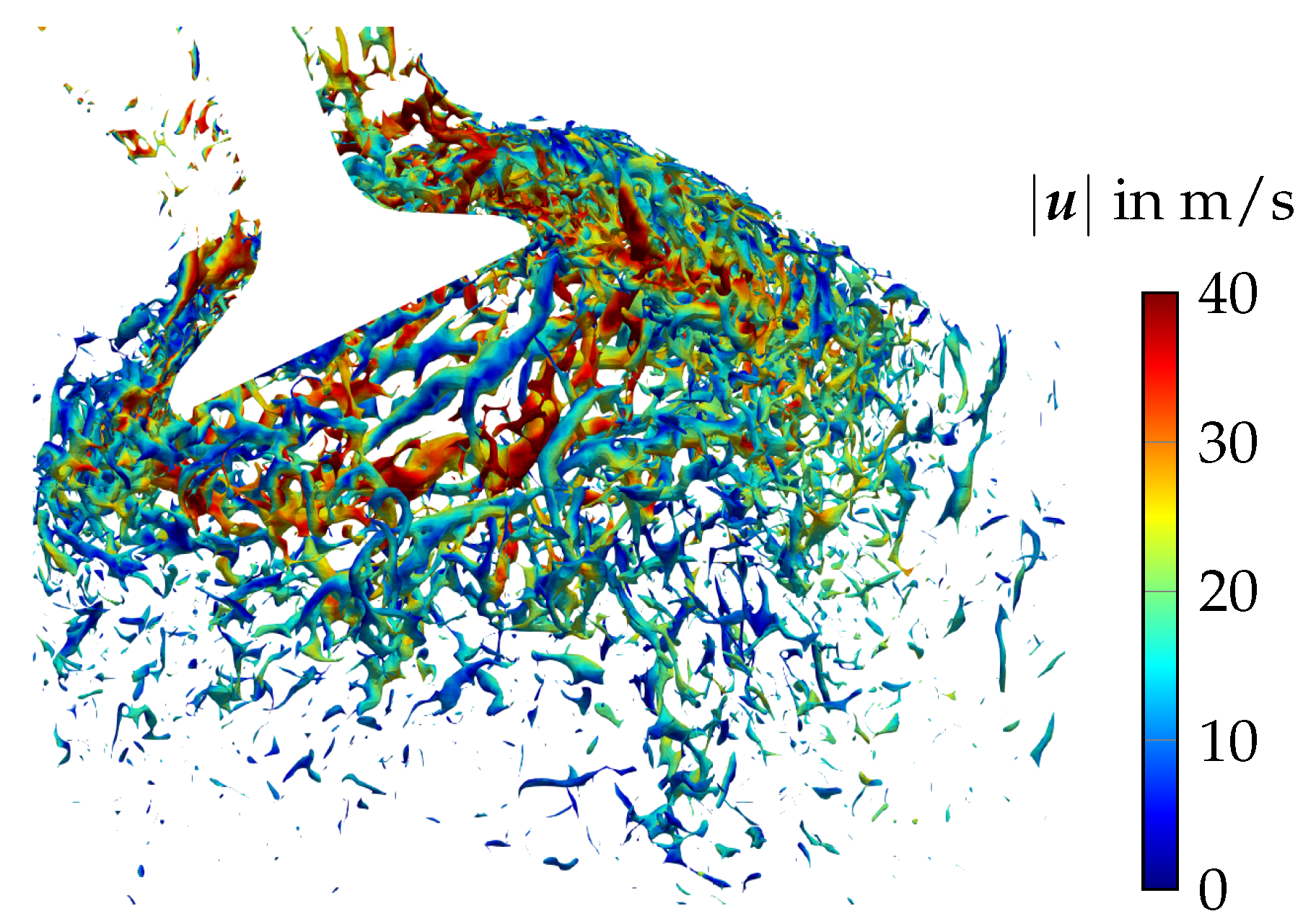
4.1. Characterization of the In-Cylinder Flow

Figure 6 depicts the magnitude of the two dimensional time-averaged velocity $\left|\langle U\rangle \right|$ at the VP section obtained from (a) PIV measurements, (b) OpenLB and (c) OpenFOAM. Whereby $\left|\langle U\rangle \right|$ is defined by means of the in-plane velocity components as

$$\left|\langle U\rangle \right|=\sqrt{{\langle u_x\rangle }^2+{\langle u_y\rangle }^2}.$$

(42)

The absence of the plane normal components is due to the two-dimensional PIV measurement data (see Section 3.1).

Characterized by strong flow/wall interaction processes, the turbulent flow inside IC engines features very complex flow and mixing dynamics. Considering Figure 6, some of the complex types of flow relevant to IC engines can also be found in the flow bench configuration; namely, (I) boundary layer flow, (II) impingement/stagnation, (III) wall-jets, (IV) flow separation/reattachment and (V) the so-called tumble flow. By comparing the LES results with the PIV measurements in Figure 6, it appears that LBM as well as FVM are able to properly predict such flow types. Furthermore, it can be clearly seen that predictions of LBM and FVM are quite similar to each other and also generally similar to the PIV measurements. This confirms the validity of LBM and FVM for such a fluid flow application.

The complex physics of engine flows are further analyzed and highlighted in Figure 7, which shows a snapshot of turbulent structures in the vicinity of the valve visualized by means of the Q-criterion [71]. Thereby, iso-surfaces of $Q=7\times {10}^{-7}$ are colored by the magnitude of the instantaneous velocity.

As is visible in Figure 7, a highly turbulent flow is generated around the intake valve. This gas stream separates from the valve and initiates large-scale turbulent structures, which cascade into smaller ones until they dissipate further downstream. Such a complex disintegration process is essential in the context of IC engine flows since it influences the mixing and subsequent flow pattern inside the combustion chamber. It is nearly impossible to capture these three dimensional turbulent scales experimentally. However, as seen in Figure 7, it can be well represented by means of LBM and FVM techniques.

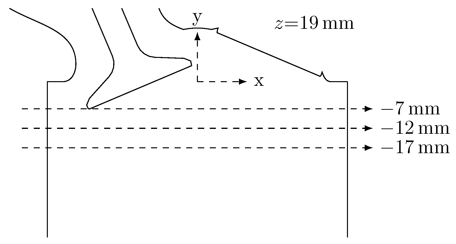
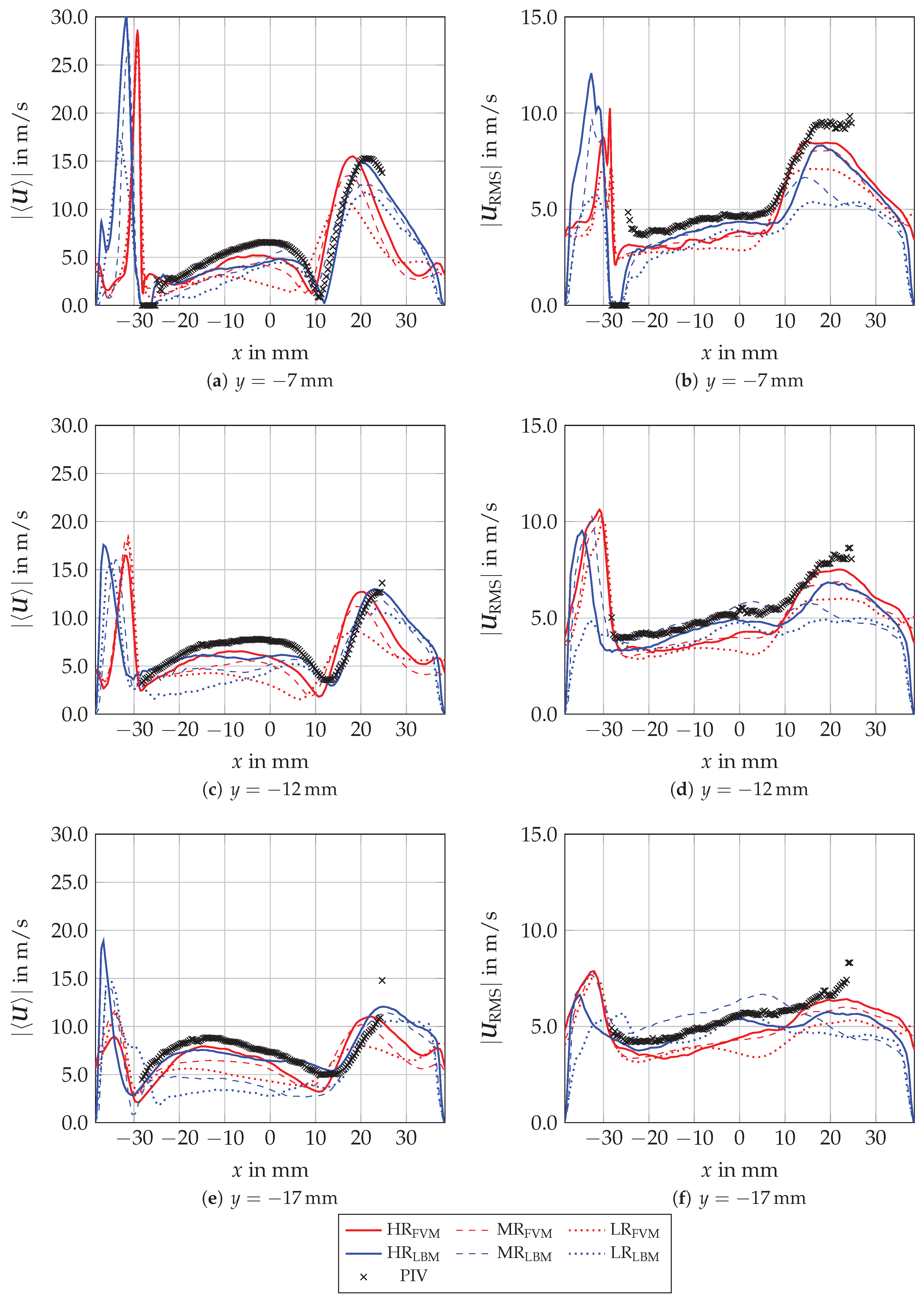
4.2. Validation of In-Cylinder Fluid Flow

For further comparison, the magnitudes for the two-dimensional time-averaged velocity $\left|\langle U\rangle \right|$ and RMS velocity $\left|U_{\mathrm{RMS}}\right|$ are plotted over three lines positioned at $y=-7\mathrm{mm}$, $-12\mathrm{mm}$ and $-17\mathrm{mm}$, see Figure 8.

The magnitude for the two-dimensional RMS velocity vector is again obtained from the two in-plane components

$$\left|U_{\mathrm{RMS}}\right|=\sqrt{u_{\mathrm{RMS},x}^2+u_{\mathrm{RMS},y}^2}.$$

(43)

For these three lines, each grid configuration of both solvers and the PIV results are presented in Figure 9.

It can be seen that the highest grid resolutions ${\mathrm{HR}}_{\mathrm{LBM}}$ and ${\mathrm{HR}}_{\mathrm{FVM}}$ agree well with the trends of the PIV results. Furthermore, the different convergence behaviors in the near-wall region are observable. Due to the used grid refinement, the wall jet can be described more precisely by ${\mathrm{LR}}_{\mathrm{FVM}}$ and ${\mathrm{MR}}_{\mathrm{FVM}}$ compared with ${\mathrm{LR}}_{\mathrm{LBM}}$ and ${\mathrm{MR}}_{\mathrm{LBM}}$. In contrast, OpenLB is able to predict the transition area of the tumble flow to the right-side wall jet more accurately than OpenFOAM, even with the lower resolutions ${\mathrm{LR}}_{\mathrm{LBM}}$ and ${\mathrm{MR}}_{\mathrm{LBM}}$.

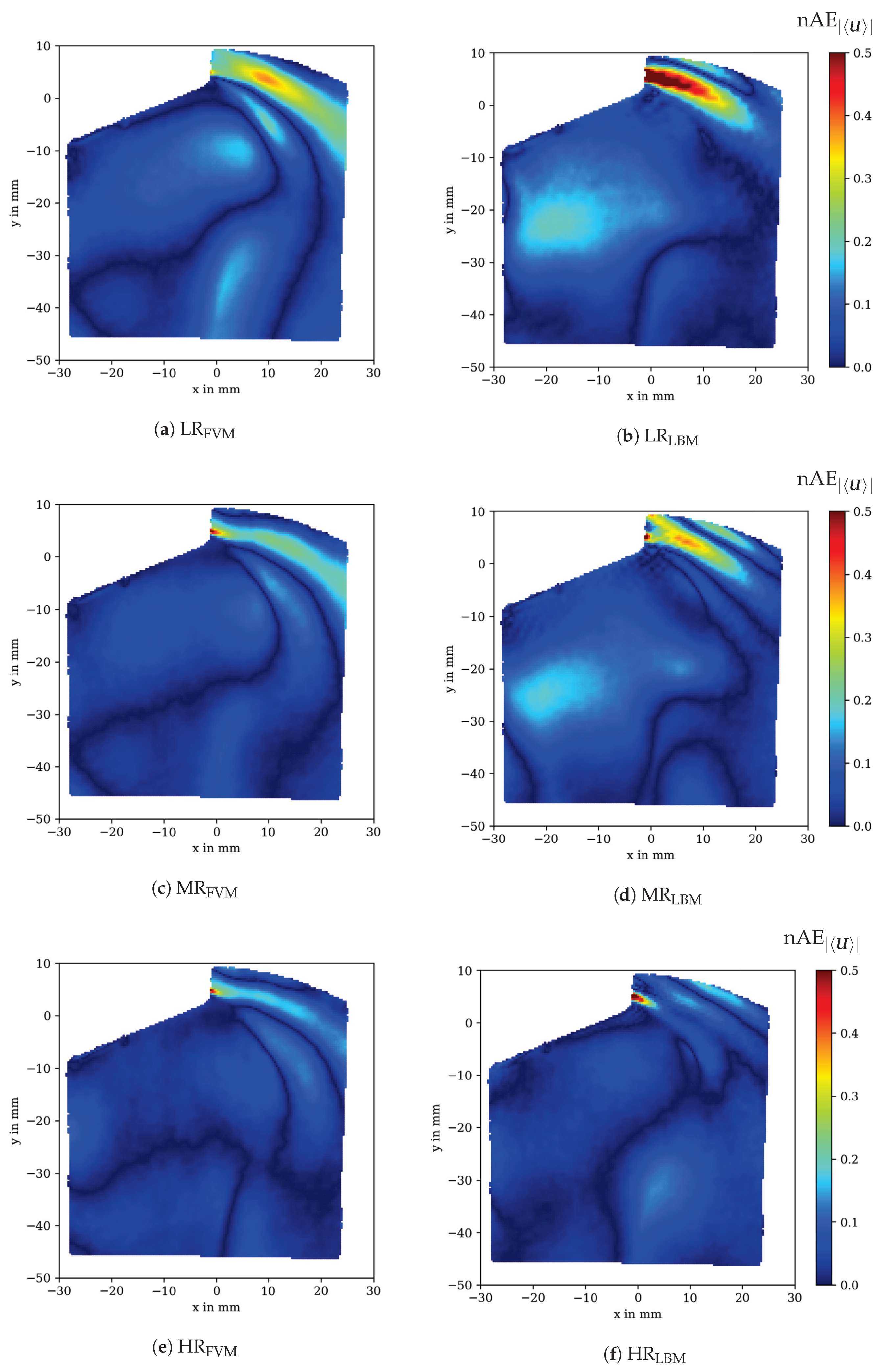
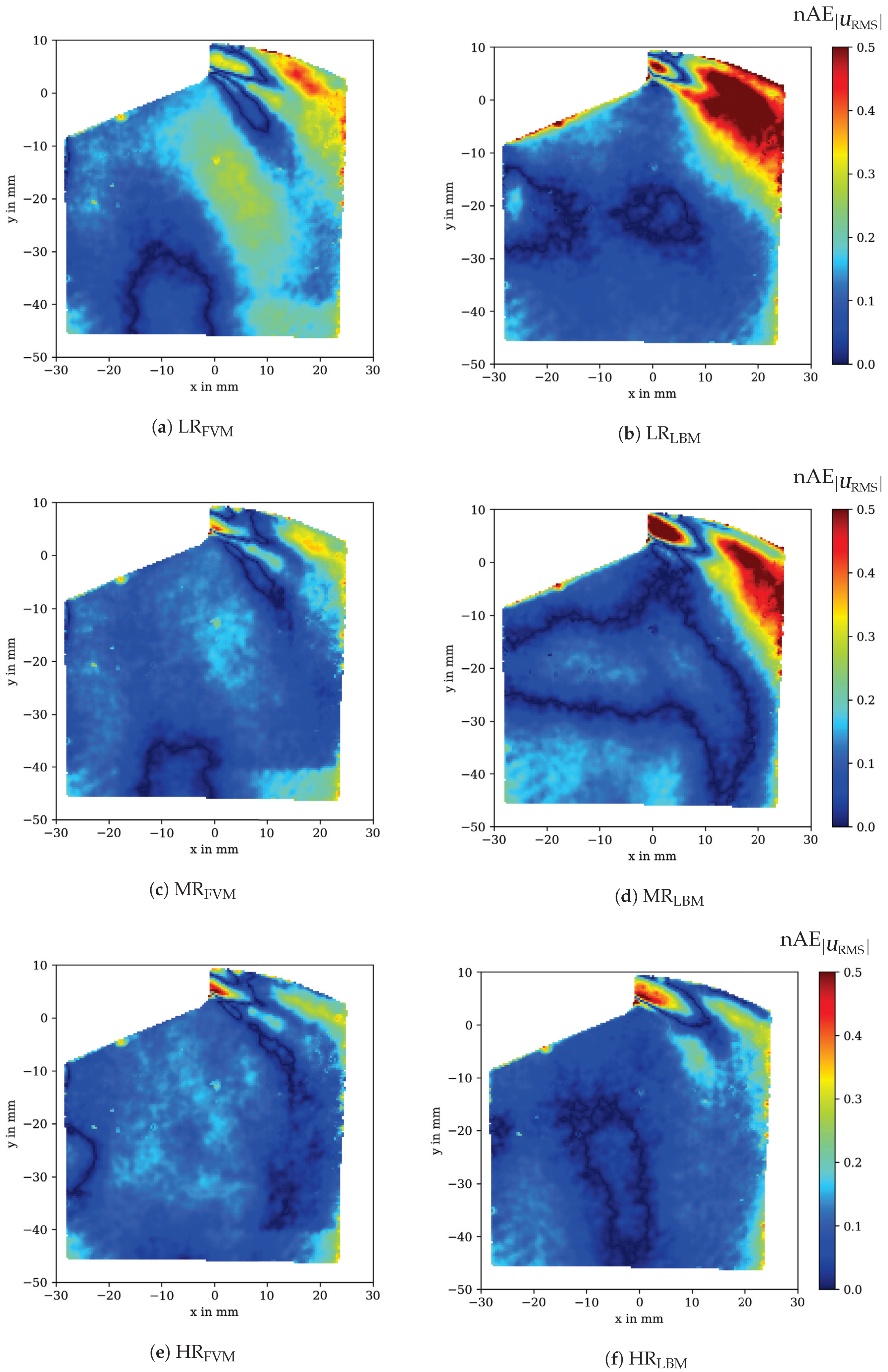
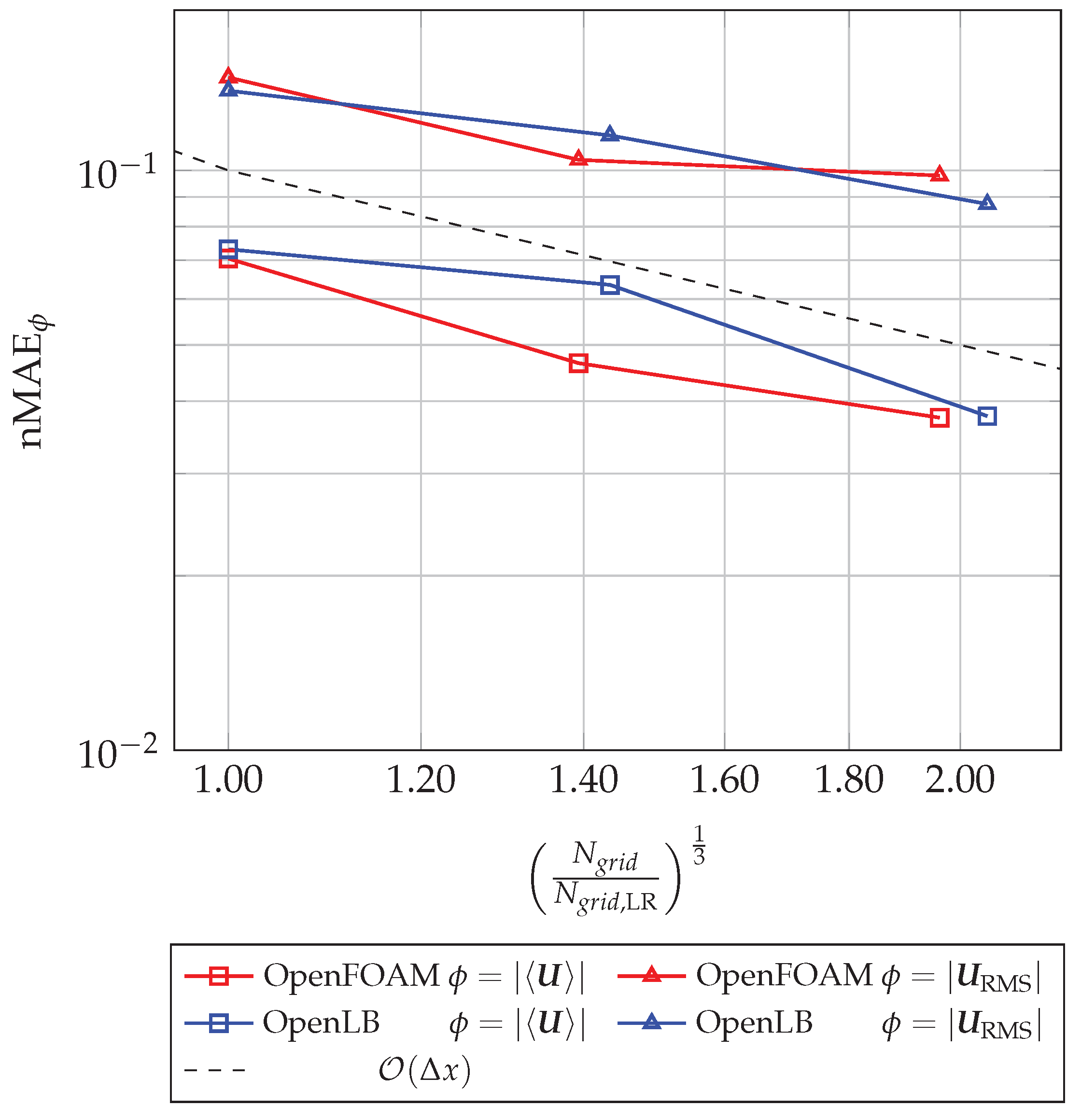
4.3. Prediction Accuracy

The prediction accuracy of the numerical results calculated by OpenLB and OpenFOAM is compared with each other by means of the PIV measurement data. Therefore, we introduce the normalized absolute error nAE as the error criterion. The nAE for variable $\varphi$ at position $x$ is defined as

$${\mathrm{nAE}}_{\varphi }\left(x\right)=\frac{|{\varphi }_{sim}\left(x\right)-{\varphi }_{\mathrm{PIV}}\left(x\right)|}{max\left({\varphi }_{\mathrm{PIV}}\left(x\right)\right)-min\left({\varphi }_{\mathrm{PIV}}\left(x\right)\right)},$$

(44)

where ${\varphi }_{sim}$ is the simulated data and ${\varphi }_{\mathrm{PIV}}$ is the PIV measurement data, which is used as the reference value. The normalization is obtained by the interval length of the experimental data. The ${\mathrm{nAE}}_{\left|\langle U\rangle \right|}$, concerning the time-averaged velocity $\left|\langle U\rangle \right|$, is depicted for the three different grid resolutions LR, MR and HR in Figure 10. The region of interest is in accordance with the experimental data (VP, see Figure 3 and Figure 8).

For the low grid resolution LR, both OpenFOAM and OpenLB show the largest errors in the jet region (see Figure 10a,b. Also, the tumble flow prediction accuracy is diminished in comparison with higher grid resolutions. It can be observed that especially the approximation of the jet region in ${\mathrm{LR}}_{\mathrm{LBM}}$ is worse than ${\mathrm{LR}}_{\mathrm{FVM}}$, due to the larger grid spacing in the near-wall region around the valve. In contrast, the medium grid resolution exhibits in both cases that the error in the jet region is reduced (see Figure 10c,d. The high deviation region at the starting point of the jet is related to a shifted separation point of the boundary layer on the valve surface. Overall, the flow field of ${\mathrm{MR}}_{\mathrm{FVM}}$ approximates the PIV measurement data better than ${\mathrm{MR}}_{\mathrm{LBM}}$, which is due to the higher accuracy in the jet and tumble flow range. In Figure 10e,f, the error maps for the highest grid resolution are presented. The error maps for ${\mathrm{HR}}_{\mathrm{LBM}}$ and ${\mathrm{HR}}_{\mathrm{FVM}}$ are in good agreement with each other and to the PIV measurement. Both the jet and the tumble flow region are well predicted. Again, it is noticeable that the highest deviation in the jet region is related to a shifted separation point.

For the RMS velocity $\left|U_{\mathrm{RMS}}\right|$, high errors are more spread over the jet region compared with the mean velocity $\left|\langle U\rangle \right|$ errors, reaching into the tumble region as the fluctuation due to turbulent kinetic energy is amplified by the velocity (see Figure 11). For both LR and MR, OpenFOAM is able to predict the turbulent velocity fluctuations in the jet region better than OpenLB as a result of the graded mesh (see Figure 11a–d). For the same reason, OpenLB shows much smaller errors in the tumble region, while OpenFOAM suffers from greater errors at ${\mathrm{MR}}_{\mathrm{FVM}}$ and ${\mathrm{LR}}_{\mathrm{FVM}}$ (see Figure 11a,c). Similar to the $\left|\langle U\rangle \right|$ error map, $\left|U_{\mathrm{RMS}}\right|$ is in good agreement with the PIV measurements for ${\mathrm{HR}}_{\mathrm{LBM}}$ and ${\mathrm{HR}}_{\mathrm{FVM}}$ given in Figure 11e,f.

A global error criterion can be defined by the arithmetic mean of the normalized error ${\mathrm{nAE}}_{\varphi }$. This normalized mean absolute error ${\mathrm{nMAE}}_{\varphi }$ is given by

$${\mathrm{nMAE}}_{\varphi }=\frac{1}{N_{\mathrm{PIV}}}\sum _{k=1}^{N_{\mathrm{PIV}}}{\mathrm{nAE}}_{\varphi }\left(x_k\right),$$

(45)

where $N_{\mathrm{PIV}}$ is the number of experimental data points in the plane. Figure 12 depicts the normalized mean absolute error of the mean velocity ${\mathrm{nMAE}}_{\left|\langle U\rangle \right|}$ and the RMS velocity ${\mathrm{nMAE}}_{\left|U_{\mathrm{RMS}}\right|}$.

It can be seen that the nMAE decreases with an increasing number of cells. Both errors for the time-averaged velocity and the RMS velocity are lower than ${\mathrm{nMAE}}_{\left|\langle U\rangle \right|}<0.08$ and ${\mathrm{nMAE}}_{\left|U_{\mathrm{RMS}}\right|}<0.15$, respectively, which is satisfactory for such coarse meshes. The errors for the highest resolution are very similar, which is also indicated by the corresponding error maps (see Figure 10e,f). The convergence order for the OpenLB and OpenFOAM configurations is lower than the first order. This diminished convergence order can be justified by the experimental reference data, where the estimated PIV measurement uncertainty is ${\mathrm{nMAE}}_{\left|\langle U\rangle \right|}=0.01$. Another source of error for the RMS velocity, besides the uncertainty of the PIV data, is the sampling error ${ϵ}_{\mathrm{RMS}}=0.025$. This may also affect the convergence order of ${\mathrm{nMAE}}_{\left|U_{\mathrm{RMS}}\right|}$.

4.4. Computational Cost

Besides the accuracy, the computational costs are a key factor to analyze the suitability of a numerical method. Therefore, the runtime of the mesh generation and the solver was evaluated on a single node which consists of two dodeca-core Intel Xeon processors E5-2680 v3 that support AVX2. The node provides 64 GB main memory. The use of a single node for estimating runtime performance was chosen because the parallel scalability is not in the scope of this study. The estimation of parallel scalability requires extensive testing due to the strong influence by the cells per core ratio, the load balancing method and the connection between the nodes of the cluster system. Comprehensive studies that deal with the parallel scalability of OpenFOAM and OpenLB can be found in [43,72,73].

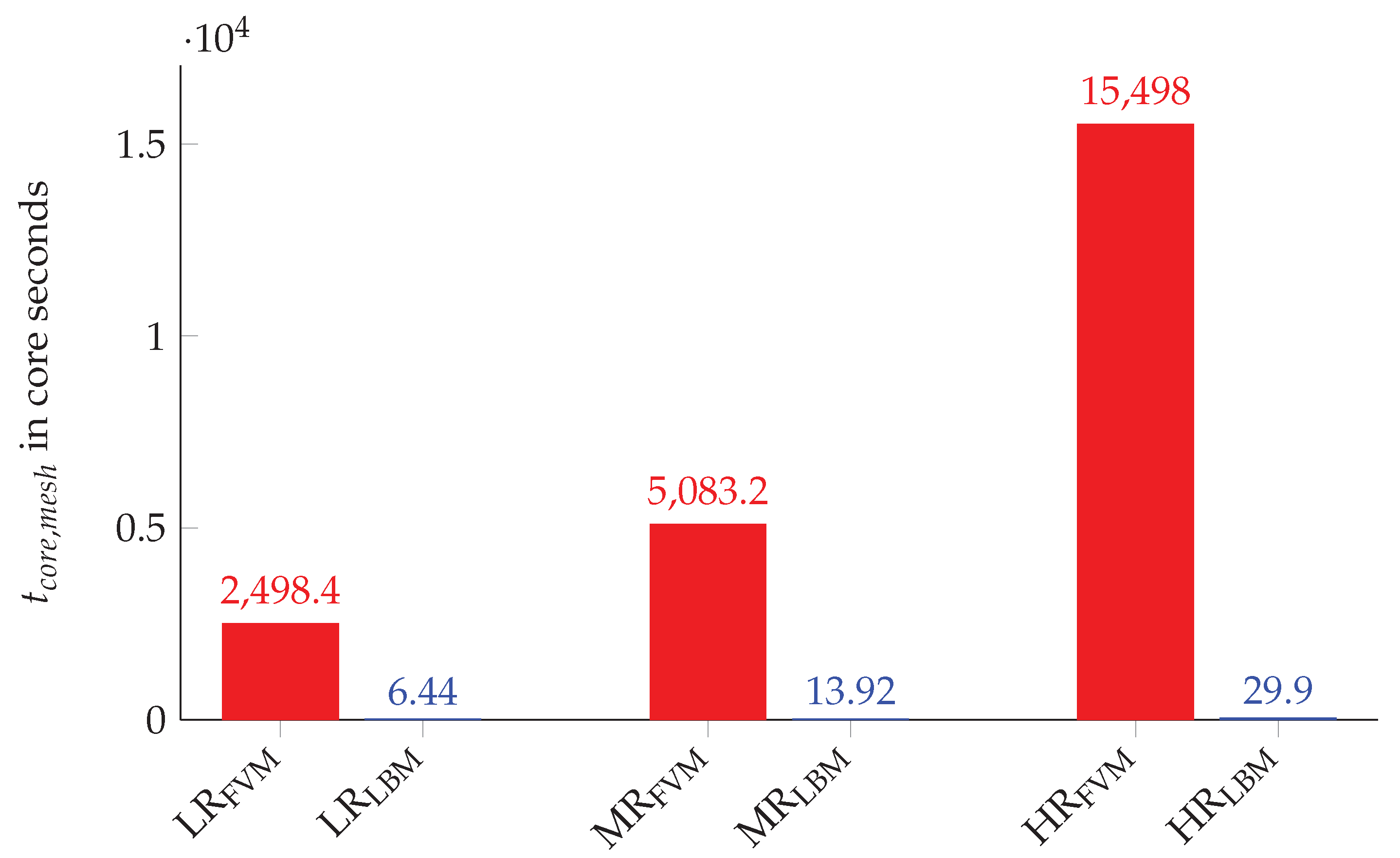
4.4.1. Meshing Performance

Due to the straightforward approach in the case of OpenLB, the grid generation is fully automatic and does not require any additional preparation steps. On the contrary, the meshing process for FVM is very time-consuming if the grid is manually obtained. Internal OpenFOAM tools can drastically reduce the effort, but require an experienced user. This study uses the built-in OpenFOAM meshing tool snappyHexMesh. Still, writing a script for grid generation for a complex geometry can take several days. Nevertheless, we only take the runtime for the mesh generation into account. The meshing time is estimated by

$$t_{core,mesh}=N_{core}{t}_{node,mesh},$$

(46)

where $t_{node,mesh}$ is the runtime on the node and $N_{core}$ the amount of used cores. The comparison of the meshing time for the three different resolutions is represented in Figure 13.

It can be observed that the meshing time in OpenLB is more than doubled each time the higher grid resolution is used. In contrast, the results of OpenFOAM show a certain overhead with the high resolution grid, i.e. The grid generation for OpenFOAM takes considerably more time with each increase in resolution. This can be justified by the complex meshing procedure, which consists of a castellation, snapping and adding layers step including several optimization cycles. Overall, the meshing time in OpenLB is on average 424 times shorter than in OpenFOAM. In the case of a static mesh, this performance benefit is not decisive. However, the use of a moving mesh, e.g., if piston motions are taken into account, requires several mesh updates in one cycle. Therefore, a fast grid creation process, such as that with OpenLB, can be essential in the context of engine relevant flows. The suitability of LBM for describing moving boundaries has been demonstrated in extensive comparisons for different moving boundary methods, e.g., in [74,75].

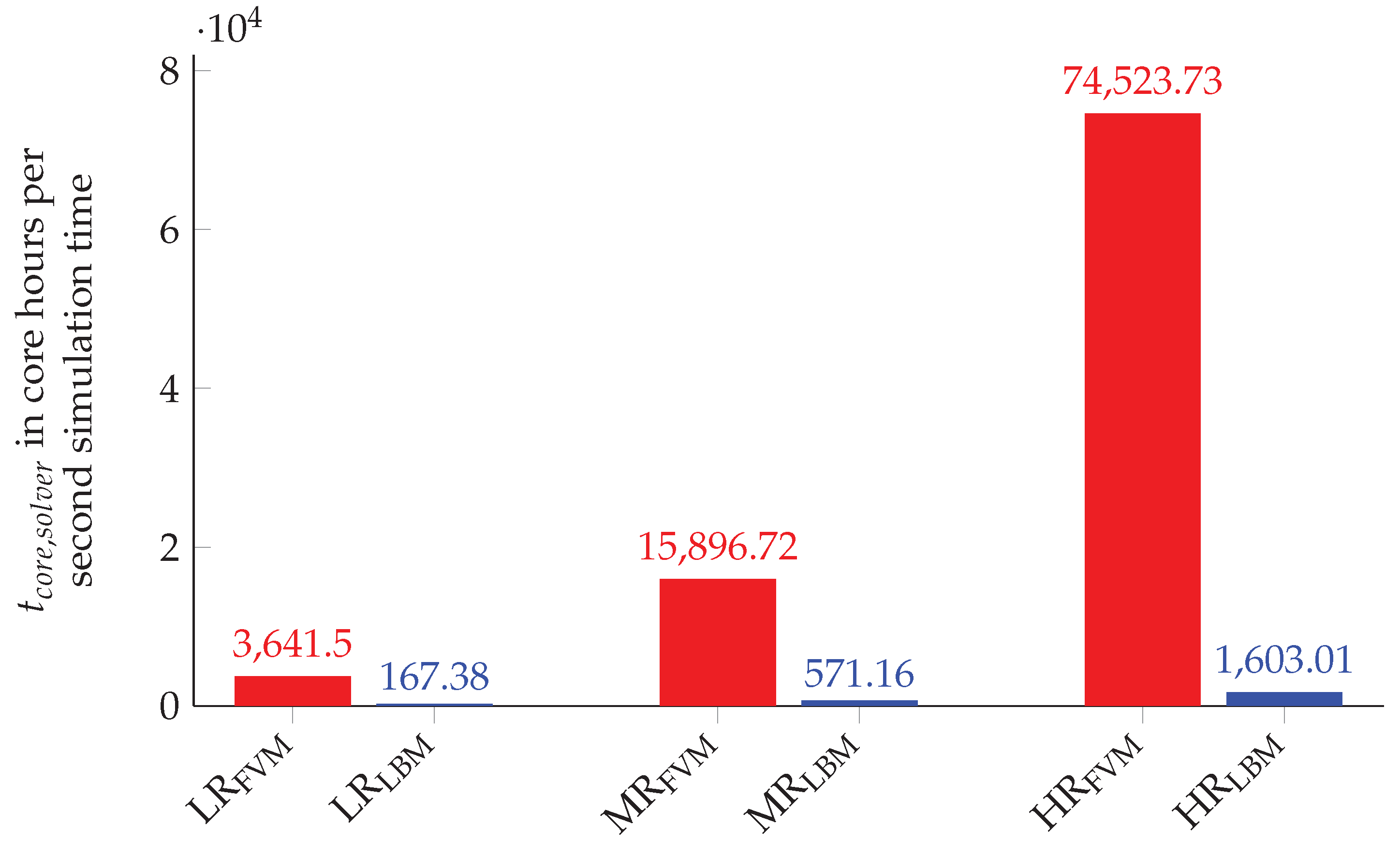
4.4.2. Simulation Performance

For the comparison of the simulation performance difference for each grid, a runtime metric is introduced. At $t_{ss}=0.5\mathrm{s}$, the beginning of the statistics computation, the runtime tracker is started. The tracked runtime $t_{node,solver}$ is divided by the according past simulation time $t_{sim,solver}$ and scaled with the number of cores $N_{core}$. This core time $t_{core,solver}$ is written as

$$t_{core,solver}=\frac{N_{core}{t}_{node,solver}}{t_{sim,solver}}.$$

(47)

This means that the runtime metric calculates the core hours for one second of simulation time including the additional time for processing the turbulence statistics. The direct comparison of each grid resolution is justified by the comparable accuracy, see Section 4.3. The performance results for the three different grid resolutions are presented in Figure 14.

The bar chart reveals that the simulations obtained by OpenLB are significantly faster than the OpenFOAM simulations. The resulting performance factor can be determined by dividing $t_{core,solver}$ for the corresponding grid resolutions. If each grid configuration is taken into account, the mean performance factor for OpenLB to OpenFOAM can be estimated as $32.03$. It is noteworthy that the performance factor varies greatly between the different grid resolutions, $21.76$ for LR and $46.49$ for HR. Additional quantities are introduced to further investigate the variance of the performance factor. The mean cells per core (MCPc) are given by

$$\mathrm{MCPc}=\frac{N_{grid}}{N_{core}}.$$

(48)

Another performance metric are the cell updates per core and second (CUPcs), which are defined as

$$\mathrm{CUPcs}=\frac{N_{grid}}{t_{core,solver}\Delta t}.$$

(49)

Both quantities MCPc and CUPcs are listed for the three grid configurations in

Table 3. Mean cells per core (MCPc) and cell updates per core and second (CUPcs) for the three grid configurations: low resolution (LR), medium resolution (MR) and high resolution (HR) for both OpenFOAM and OpenLB

Solver	Identifier	MCPc	CUPcs
OpenFOAM	${\mathrm{LR}}_{\mathrm{FVM}}$	$5.016\times {10}^4$	$2.934\times {10}^4$
OpenFOAM	${\mathrm{MR}}_{\mathrm{FVM}}$	$1.357\times {10}^5$	$2.424\times {10}^4$
OpenFOAM	${\mathrm{HR}}_{\mathrm{FVM}}$	$3.788\times {10}^5$	$2.023\times {10}^4$
OpenLB	${\mathrm{LR}}_{\mathrm{LBM}}$	$5.654\times {10}^4$	$1.208\times {10}^6$
OpenLB	${\mathrm{MR}}_{\mathrm{LBM}}$	$1.672\times {10}^5$	$1.521\times {10}^6$
OpenLB	${\mathrm{HR}}_{\mathrm{LBM}}$	$4.885\times {10}^5$	$2.283\times {10}^6$

.

The solvers show a contrary behavior, while OpenLB benefits from an increased MCPc and almost doubles the CUPcs from LR to HR, OpenFOAM has a decrease of about 45 percent. Consequently, OpenFOAM seems to be less affected by the used MCPc. The reasons for the different behavior can be manifold and range from the influence of the load balancing method to cache effects and communication effects. A detailed discussion of these influencing factors can be found in [72,76,77].

5. Conclusions and Outlook

The purpose of this paper is to evaluate NWM-LES for complex turbulent flows using LBM by comparison with FVM simulations and PIV experiments. Thereby, a van Driest damped Smagorinsky model coupled to the Musker equation was used to model the turbulent boundary layer. Both LBM and FVM NWM-LES approaches were outlined in detail. Three different grid resolutions were used to simulate an engine relevant in-cylinder flow with the open source frameworks OpenLB and OpenFOAM. Characteristic flow features of the in-cylinder flow were highlighted and compared side-by-side. In addition to the quantitative comparison, the errors of the tested grid configuration were calculated against a highly precise PIV measurement and analyzed in detail. It was shown that the matching grid configurations of both numerical methods had similar errors. Surprisingly, OpenLB requires only slightly more cells than OpenFOAM to produce the same accuracy, although no grid refinement was used. This can be justified by the chosen region of interest, which is remote from the wall, and also the incorporated near-wall treatment based on the wall function approach. The time-averaged and the RMS velocity at the highest grid resolution for OpenLB and OpenFOAM were in good agreement with the PIV measurement (${\mathrm{nMAE}}_{\left|\langle U\rangle \right|}<0.038$ and ${\mathrm{nMAE}}_{\left|U_{\mathrm{RMS}}\right|}<0.098$, respectively). The performance estimation revealed that the meshing process in OpenLB was 424 times faster and the simulation process approximately 32 times faster for the investigated setup. These significant performance differences in meshing and solver runtime indicate that LBM is a valuable and viable alternative to FVM in simulating IC engine relevant flows with NWM-LES. In particular, the fast grid generation process in OpenLB further reduces computational costs, if moving meshes are applied. The faster calculation speed for NWM-LES using LBM is advantageous to address industrial applications and to enable "overnight" calculations that previously took weeks. Therefore, faster design cycles and operating condition tests are feasible. The performance advantage can also be used to provide more precise results in the same time and finally paves the way for near-wall-resolved LES in the future [78].

Nevertheless, LBM still needs additional research to gain the maturity of NWM-LES with FVM. The applied equilibrium wall function approach based on Musker’s law of the wall is strictly speaking only valid in fully developed turbulent boundary layers. In contrast, turbulent boundary layers of complex turbulent flows deal with pressure gradients, separation and recirculation, variable physical properties, compressibility effects and many more. Therefore, a further step is to implement a generalized wall function such as [79,80,81] in OpenLB that is able to model these flow features. In addition, the simple SGS model employed in this study can be replaced by more advanced turbulent models, e.g., models based on dynamic procedures [82], the scale similarity hypothesis [83] or wall-adapted SGS models [52], which have shown an increased accuracy for IC engine flows [2,42]. If reactive turbulent flows are considered, further investigations have to be done. In this respect, a modeling approach based on detailed chemistry with a large number of species as well as tabulated chemistry is a challenging task, especially for LBM due to the high memory requirements [84]. However, given the benefits of the mesh generation and computation time reductions shown in this work, LBM is a promising alternative to FVM in IC engine and many other complex turbulent flow applications in the future.

References

1. Freudenhammer, D.; Baum, E.; Peterson, B.; Böhm, B.; Jung, B.; Grundmann, S. Volumetric intake flow measurements of an IC engine using magnetic resonance velocimetry. Exp. Fluids 2014, 55, 1724. [Google Scholar] [CrossRef]
2. Rutland, C. Large-eddy simulations for internal combustion engines—A review. Int. J. Eng. Res. 2011, 12, 421–451. [Google Scholar] [CrossRef] [Green Version]
3. Vermorel, O.; Richard, S.; Colin, O.; Angelberger, C.; Benkenida, A.; Veynante, D. Towards the understanding of cyclic variability in a spark ignited engine using multi-cycle LES. Combust. Flame 2007, 1525–1541. [Google Scholar] [CrossRef]
4. Goryntsev, D.; Sadiki, A.; Klein, M.; Janicka, J. Large eddy simulation based analysis of the effects of cycle-to-cycle variations on air-fuel mixing in realistic DISI engines. Proc. Combust. Inst. 2009, 2759–2766. [Google Scholar] [CrossRef]
5. Enaux, B.; Granet, V.; Vermorel, O.; Lacour, C.; Thobois, L.; Dugué, V.; Poinsot, T. Large eddy simulation of a motored single-cylinder piston engine: Numerical strategies and validation. Flow Turbul. Combust. 2010, 53–177. [Google Scholar] [CrossRef]
6. Granet, V.; Vermorel, O.; Lacour, C.; Enaux, B.; Dugué, V.; Poinsot, T. Large-Eddy Simulation and experimental study of cycle-to-cycle variations of stable and unstable operating points in a spark ignition engine. Combust. Flame 2012, 1562–11575. [Google Scholar] [CrossRef] [Green Version]
7. Goryntsev, D.; Nishad, K.; Sadiki, A.; Janicka, J. Application of LES for analysis of unsteady effects on combustion processes and misfires in DISI engine. Oil Gas Sci. Technol. Revue d’IFP Energies Nouvelles 2014, 129–140. [Google Scholar] [CrossRef] [Green Version]
8. Reuss, D.L.; Adrian, R.J.; Landreth, C.C.; French, D.T.; Fansler, T.D. Instantaneous planar measurements of velocity and large-scale vorticity and strain rate in an engine using particle-image velocimetry. SAE Trans. 1989, 1116–1141. [Google Scholar]
9. Peterson, B.; Sick, V. Simultaneous flow field and fuel concentration imaging at 4.8 kHz in an operating engine. Appl. Phys. B 2009, 97, 887. [Google Scholar] [CrossRef]
10. Baum, E.; Peterson, B.; Böhm, B.; Dreizler, A. On the validation of LES applied to internal combustion engine flows: Part 1: Comprehensive experimental database. Flow Turbul. Combust. 2014, 92, 269–297. [Google Scholar] [CrossRef]
11. Zentgraf, F.; Baum, E.; Böhm, B.; Dreizler, A.; Peterson, B. On the turbulent flow in piston engines: Coupling of statistical theory quantities and instantaneous turbulence. Phys. Fluids 2016, 28, 045108. [Google Scholar] [CrossRef] [Green Version]
12. Gale, N.F. Diesel engine cylinder head design: The compromises and the techniques. SAE Trans. 1990, 415–438. [Google Scholar] [CrossRef]
13. Agnew, D.D. What is Limiting your Engine Air Flow: Using Normalized Steady Air Flow Bench Data; Technical Report, SAE Technical Paper; SAE: Warrendale, PA, USA, 1994. [Google Scholar] [CrossRef]
14. Hartmann, F.; Buhl, S.; Gleiss, F.; Barth, P.; Schild, M.; Kaiser, S.A.; Hasse, C. Spatially resolved experimental and numerical investigation of the flow through the intake port of an internal combustion engine. Oil Gas Sci. Technol. Revue d’IFP Energies Nouvelles 2016, 71, 2. [Google Scholar] [CrossRef] [Green Version]
15. Falkenstein, T.; Bode, M.; Kang, S.; Pitsch, H.; Arima, T.; Taniguchi, H. Large-Eddy Simulation study on unsteady effects in a statistically stationary SI engie port flow. SAE Int. 2015. [Google Scholar] [CrossRef]
16. Buhl, S.; Hartmann, F.; Kaiser, S.A.; Hasse, C. Investigation of an IC engine intake flow based on highly resolved LES and PIV. Oil Gas Sci. Technol. Revue d’IFP Energies Nouvelles 2017, 72, 15. [Google Scholar] [CrossRef] [Green Version]
17. Falkenstein, T.; Kang, S.; Davidovic, M.; Bode, M.; Pitsch, H.; Kamatsuchi, T.; Nagao, J.; Arima, T. LES of Internal Combustion Engine Flows Using Cartesian Overset Grids. Oil Gas Sci. Technol.–Revue d’IFP Energies Nouvelles 2017, 72, 36. [Google Scholar] [CrossRef] [Green Version]
18. Nishad, K.; Ries, F.; Li, Y.; Sadiki, A. Numerical Investigation of Flow through a Valve during Charge Intake in a DISI-Engine using Large Eddy Simulation. Energies 2019, 12, 2620. [Google Scholar] [CrossRef] [Green Version]
19. Gaedtke, M.; Hoffmann, T.; Reinhardt, V.; Thäter, G.; Nirschl, H.; Krause, M.J. Flow and heat transfer simulation with a thermal large eddy lattice Boltzmann method in an annular gap with an inner rotating cylinder. Int. J. Modern Phys. C 2019, 30, 1950013. [Google Scholar] [CrossRef]
20. Gaedtke, M.; Wachter, S.; Kunkel, S.; Sonnick, S.; Rädle, M.; Nirschl, H.; Krause, M.J. Numerical study on the application of vacuum insulation panels and a latent heat storage for refrigerated vehicles with a large Eddy lattice Boltzmann method. Heat Mass Transf. 2020, 56, 1189–1201. [Google Scholar] [CrossRef]
21. Augusto, L.d.L.X.; Ross-Jones, J.; Lopes, G.C.; Tronville, P.; Gonçalves, J.A.S.; Rädle, M.; Krause, M.J. Microfiber filter performance prediction using a lattice Boltzmann method. Commun. Comput. Phys. 2018, 23, 910–931. [Google Scholar] [CrossRef]
22. Henn, T.; Heuveline, V.; Krause, M.J.; Ritterbusch, S. Aortic Coarctation Simulation Based on the Lattice Boltzmann Method: Benchmark Results. In Statistical Atlases and Computational Models of the Heart. Imaging and Modelling Challenges; Camara, O., Mansi, T., Pop, M., Rhode, K., Sermesant, M., Young, A., Eds.; Springer: Berlin/Heidelberg, Germany, 2013; pp. 34–43. [Google Scholar]
23. Heuveline, V.; Krause, M.J.; Latt, J. Towards a hybrid parallelization of lattice Boltzmann methods. Comput. Math. Appl. 2009, 58, 1071–1080. [Google Scholar] [CrossRef] [Green Version]
24. Heuveline, V.; Krause, M.J. OpenLB: Towards an efficient parallel open source library for lattice Boltzmann fluid flow simulations. In International Workshop on State-of-the-Art in Scientific and Parallel Computing; PARA: Trondheim, Norway, 2010; Volume 9. [Google Scholar]
25. Kajzer, A.; Pozorski, J.; Szewc, K. Large-eddy simulations of 3D Taylor-Green vortex: Comparison of smoothed particle hydrodynamics, lattice Boltzmann and finite volume methods. J. Phys. Conf. Ser. 2014, 530, 012019. [Google Scholar] [CrossRef] [Green Version]
26. Pasquali, A.; Schönherr, M.; Geier, M.; Krafczyk, M. Simulation of external aerodynamics of the DrivAer model with the LBM on GPGPUs. In Parallel Computing: On the Road to Exascale; IOS Press: Amsterdam, The Netherlands, 2016; Volume 27, pp. 391–400. [Google Scholar] [CrossRef]
27. Jin, Y.; Uth, M.; Herwig, H. Structure of a turbulent flow through plane channels with smooth and rough walls: An analysis based on high resolution DNS results. Comput. Fluids 2015, 107, 77–88. [Google Scholar] [CrossRef]
28. Barad, M.F.; Kocheemoolayil, J.G.; Kiris, C.C. Lattice Boltzmann and Navier-stokes cartesian cfd approaches for airframe noise predictions. In Proceedings of the 23rd AIAA Computational Fluid Dynamics Conference, Denver, CO, USA, 5–9 June 2017; p. 4404. [Google Scholar]
29. Montessori, A.; Falcucci, G. Lattice Boltzmann Modeling of Complex Flows for Engineering Applications; Morgan & Claypool Publishers: San Rafael, CA, USA, 2018. [Google Scholar]
30. Dorschner, B.; Bösch, F.; Chikatamarla, S.S.; Boulouchos, K.; Karlin, I.V. Entropic multi-relaxation time lattice Boltzmann model for complex flows. J. Fluid Mech. 2016, 801, 623–651. [Google Scholar] [CrossRef]
31. Krause, M.; Avis, S.; Dapalo, D.; Hafen, N.; Haußmann, M.; Gaedtke, M.; Klemens, F.; Kummerländer, A.; Maier, M.L.; Mink, A.; et al. OpenLB Release 1.3: Open Source Lattice Boltzmann Code. 2019. Available online: http://optilb.com/openlb/wp-content/uploads/2011/12/olb_ug-0.5r0.pdf (accessed on 30 April 2020).
32. Malaspinas, O.; Sagaut, P. Wall model for large-eddy simulation based on the lattice Boltzmann method. J. Comput. Phys. 2014, 275, 25–40. [Google Scholar] [CrossRef]
33. Haussmann, M.; Barreto, A.C.; Kouyi, G.L.; Rivière, N.; Nirschl, H.; Krause, M.J. Large-eddy simulation coupled with wall models for turbulent channel flows at high Reynolds numbers with a lattice Boltzmann method—Application to Coriolis mass flowmeter. Comput. Math. Appl. 2019, 78, 3285–3302. [Google Scholar] [CrossRef]
34. Leonard, A. Energy cascade in large-eddy simulations of turbulent fluid flows. Adv. Geophys. A 1974, 18, 237–248. [Google Scholar]
35. Hirsch, C. Numerical Computation of Internal & External Flows: Fundamentals of Computational Fluid Dynamics, 2nd ed.; John Wiley & Sons: Burlington, MA, USA, 2007. [Google Scholar]
36. Jasak, H. Error Analysis and Estimation for the Finite Volume Method with Applications to Fluid Flows. Ph.D. Thesis, University of London, London, UK, 1996. [Google Scholar]
37. Greenshields, C.J. OpenFOAM Programmer’s Guide Version 3.0.1; OpenFOAM Foundation Ltd.: England, UK, 13 December 2015. [Google Scholar]
38. Ferziger, J.; Perić, M. Computational Methods for Fluid Dynamics, 3rd ed.; Springer: Berlin/Heidelberg, Germany; New York, NY, USA, 2002. [Google Scholar]
39. Greenshields, C.; Weller, H.; Gasparini, L.; Reese, J. Implementation of semi-discrete, non-staggered central schemes in a colocated, polyhedral, finite volume framework, for high-speed viscous flows. Int. J. Numer. Meth. Fluids 2010, 63, 1–21. [Google Scholar] [CrossRef] [Green Version]
40. Issa, R. Solution of the implicitly discretised fluid flow equations by operator-splitting. J. Comput. Phys. 1985, 62, 40–65. [Google Scholar] [CrossRef]
41. Patankar, S.; Spalding, D. A calculation procedure for heat, mass and momentum transfer in three-dimensional parabolic flows. Int. J. Heat Mass Trans. 1972, 15, 1787–1806. [Google Scholar] [CrossRef]
42. Ries, F.; Nishad, K.; Dressler, L.; Janicka, J.; Sadiki, A. Evaluating large eddy simulation results based on error analysis. Theor. Comput. Fluid Dyn. 2018, 32, 733–752. [Google Scholar] [CrossRef] [Green Version]
43. Ries, F. Numerical Modeling and Prediction of Irreversibilities in Sub- and Supercritical Turbulent Near-Wall Flows. Ph.D. Thesis, Technische Universität Darmstadt, Darmstadt, Germany, 2019. [Google Scholar]
44. Kang, S.K.; Hassan, Y.A. The effect of lattice models within the lattice Boltzmann method in the simulation of wall-bounded turbulent flows. J. Comput. Phys. 2013, 232, 100–117. [Google Scholar] [CrossRef]
45. Bhatnagar, P.L.; Gross, E.P.; Krook, M. A Model for Collision Processes in Gases. I. Small Amplitude Processes in Charged and Neutral One-Component Systems. Phys. Rev. 1954, 94, 511–525. [Google Scholar] [CrossRef]
46. He, X.; Luo, L.S. Theory of the lattice Boltzmann method: From the Boltzmann equation to the lattice Boltzmann equation. Phys. Rev. E 1997, 56, 6811–6817. [Google Scholar] [CrossRef] [Green Version]
47. Shan, X.; Yuan, X.F.; Chen, H. Kinetic theory representation of hydrodynamics: A way beyond the Navier–Stokes equation. J. Fluid Mech. 2006, 550, 413–441. [Google Scholar] [CrossRef]
48. Smagorinsky, J. General circulation experiments with the primitive equations: I. The basic experiment. Mon. Weather Rev. 1963, 91, 99–164. [Google Scholar] [CrossRef]
49. Moin, P.; Kim, J. Numerical investigation of turbulent channel flow. J. Fluid Mech. 1982, 118, 341–377. [Google Scholar] [CrossRef] [Green Version]
50. Rogallo, R.S.; Moin, P. Numerical Simulation of Turbulent Flows. Annu. Rev. Fluid Mech. 1984, 16, 99–137. [Google Scholar] [CrossRef]
51. Fröhlich, J. Large Eddy Simulation Turbulenter Strömungen; Springer, B.G. Teubner Verlag/GWV Fachverlage GmbH: Wiesbaden, Gemany, 2006; Volume 1. [Google Scholar]
52. Nicoud, F.; Ducros, F. Subgrid-Scale Stress Modelling Based on the Square of the Velocity Gradient Tensor. Flow Turbul. Combust. 1999, 62, 183–200. [Google Scholar] [CrossRef]
53. Driest, E.V. On turbulent flow near a wall. J. Aeronaut. Sci. 1956, 23, 1007–1011. [Google Scholar] [CrossRef]
54. Nagib, H.M.; Chauhan, K.A. Variations of von Kármán coefficient in canonical flows. Phys. Fluids 2008, 20, 101518. [Google Scholar] [CrossRef]
55. de Villiers, E. The Potential of Large Eddy Simulation for the Modeling of Wall Bounded Flows. Ph.D Thesis, University of London, London, UK, 2006. [Google Scholar]
56. Hou, S.; Sterling, J.; Chen, S.; Doolen, G. A lattice Boltzmann subgrid model for high Reynolds number flows. arXiv 1998, arXiv:comp-gas/9401004. [Google Scholar]
57. Malaspinas, O.; Sagaut, P. Consistent subgrid scale modelling for lattice Boltzmann methods. J. Fluid Mech. 2012, 700, 514–542. [Google Scholar] [CrossRef]
58. Werner, H.; Wengle, H. Large-eddy simulation of turbulent flow over and around a cube in a plate channel. In Turbulent Shear Flows 8; Springer: Berlin/Heidelberg, Germany, 1993; pp. 155–168. [Google Scholar]
59. Musker, A. Explicit expression for the smooth wall velocity distribution in a turbulent boundary layer. AIAA J. 1979, 17, 655–657. [Google Scholar] [CrossRef]
60. Li, Y.; Ries, F.; Nishad, K.; Sadiki, A. Near-wall modeling of LES for non-equilibrium turbulent flows in an inclined impinging jet with moderate Re-number. In Proceedings of the 6th European Conference on Computational Mechanics (ECCM 6), Glasgow, UK, 11–15 June 2018. [Google Scholar]
61. Bouzidi, M.; Firdaouss, M.; Lallemand, P. Momentum transfer of a Boltzmann-lattice fluid with boundaries. Phys. Fluids 2001, 13, 3452–3459. [Google Scholar] [CrossRef]
62. Stich, G.D.; Housman, J.A.; Kocheemoolayil, J.G.; Barad, M.F.; Kiris, C.C. Application of Lattice Boltzmann and Navier-Stokes Methods to NASA’s Wall Mounted Hump. In Proceedings of the 2018 AIAA AVIATION Forum, Atlanta, GA, USA, 25–29 June 2018. [Google Scholar]
63. Freudenhammer, D.; Peterson, B.; Ding, C.P.; Boehm, B.; Grundmann, S. The influence of cylinder head geometry variations on the volumetric intake flow captured by magnetic resonance velocimetry. SAE Int. J. Engines 2015, 8, 1826–1836. [Google Scholar] [CrossRef]
64. Raffel, M.; Willert, C.E.; Wereley, S.T.; Kompenhans, J. Particle Image Velocimetry; Springer: Berlin/Heidelberg, Germany, 2007. [Google Scholar] [CrossRef]
65. Charonko, J.J.; Vlachos, P.P. Estimation of uncertainty bounds for individual particle image velocimetry measurements from cross-correlation peak ratio. Meas. Sci. Technol. 2013, 24, 065301. [Google Scholar] [CrossRef]
66. Sciacchitano, A.; Wieneke, B.; Scarano, F. PIV uncertainty quantification by image matching. Meas. Sci. Technol. 2013, 24, 045302. [Google Scholar] [CrossRef]
67. Wieneke, B. PIV uncertainty quantification from correlation statistics. Meas. Sci. Technol. 2015, 26, 074002. [Google Scholar] [CrossRef]
68. Sciacchitano, A.; Neal, D.R.; Smith, B.L.; Warner, S.O.; Vlachos, P.P.; Wieneke, B.; Scarano, F. Collaborative framework for PIV uncertainty quantification: Comparative assessment of methods. Meas. Sci. Technol. 2015, 26, 074004. [Google Scholar] [CrossRef] [Green Version]
69. Klein, M.; Sadiki, A.; Janicka, J. A digital filter based generation of inflow data for spatially developing direct numerical or large eddy simulations. J. Comput. Phys. 2003, 186, 652–665. [Google Scholar] [CrossRef]
70. Latt, J.; Chopard, B.; Malaspinas, O.; Deville, M.; Michler, A. Straight velocity boundaries in the lattice Boltzmann method. Phys. Rev. E 2008, 77, 056703. [Google Scholar] [CrossRef] [PubMed]
71. Kida, S.; Mirua, H. Identification and Analysis of Vortical Structures. Eur. J. Mech. B/Fluids 1998, 17, 471–488. [Google Scholar] [CrossRef]
72. Axtmann, G.; Rist, U. Scalability of OpenFOAM with Large Eddy Simulations and DNS on High-Performance Systems. In High Perfromance Computing in Science and Engineering; Springer: Cham, Switzerland, 2016; Volume 16, pp. 413–424. [Google Scholar] [CrossRef]
73. Krause, M.; Kummerländer, A.; Avis, S.; Kusumaatmaja, H.; Dapelo, D.; Klemens, F.; Gaedtke, M.; Hafen, N.; Mink, A.; Trunk, R.; et al. OpenLB–Open Source Lattice Boltzmann Code. 2020; submitted. [Google Scholar]
74. Chen, L.; Yu, Y.; Lu, J.; Hou, G. A comparative study of lattice Boltzmann methods using bounce-back schemes and immersed boundary ones for flow acoustic problems. Int. J. Numer. Methods Fluids 2014, 74, 439–467. [Google Scholar] [CrossRef]
75. Peng, C.; Ayala, O.M.; de Motta], J.C.B.; Wang, L.P. A comparative study of immersed boundary method and interpolated bounce-back scheme for no-slip boundary treatment in the lattice Boltzmann method: Part II, turbulent flows. Comput. Fluids 2019, 192, 104251. [Google Scholar] [CrossRef] [Green Version]
76. Pohl, T.; Kowarschik, M.; Wilke, J.; Iglberger, K.; Rüde, U. Optimization and profiling of the cache performance of parallel lattice Boltzmann codes. Parallel Process. Lett. 2003, 13, 549–560. [Google Scholar] [CrossRef]
77. Fietz, J.; Krause, M.J.; Schulz, C.; Sanders, P.; Heuveline, V. Optimized hybrid parallel lattice Boltzmann fluid flow simulations on complex geometries. In European Conference on Parallel Processing; Springer: Cham, Switzerland, 2012; pp. 818–829. [Google Scholar]
78. Slotnick, J.; Khodadoust, A.; Alonso, J.; Darmofal, D.; Gropp, W.; Lurie, E.; Mavriplis, D. CFD Vision 2030 Study: A Path to Revolutionary Computational Aerosciences; NASA Center for AeroSpace Information: Hanover, MD, USA, 2014. [Google Scholar]
79. Shih, T.H.; Povinelli, L.A.; Liu, N.S.; Chen, K.H. Generalized wall function for complex turbulent flows. In Proceedings of the 38th Aerospace Sciences, Reno, NV, USA, 10–13 January 2000. [Google Scholar]
80. Craft, T.; Gerasimov, A.; Iacovides, H.; Launder, B. Progress in the generalization of wall-function treatments. Int. J. Heat Fluid 2002, 23, 148–160. [Google Scholar] [CrossRef]
81. Popvac, M.; Hanjalic, K. Compound Wall Treatment for RANS Computation of Complex Turbulent Flows and Heat Transfer. Flow Turhul. Combust. 2007, 78, 177–202. [Google Scholar] [CrossRef] [Green Version]
82. Germano, M. A dynamic subgrid-scale eddy viscosity model. Phys. Fluids 1991, 3, 1760–1765. [Google Scholar] [CrossRef] [Green Version]
83. Bardina, J.; Ferziger, J.; Reynolds, W. Improved subgrid-scale models for large-eddy simulation. In Proceedings of the 3th Fluid and Plasmadynamics Conference, Los Angeles, CA, USA, 29 June–1 July 1970; p. 1357. [Google Scholar]
84. Frouzakis, C.E. Lattice boltzmann methods for reactive and other flows. In Turbulent Combustion Modeling; Springer: Cham, Switzerland, 2011; pp. 461–486. [Google Scholar]
Figure 1. Illustration of the indexing convention for the curved wall function approach applied in this work.
Computation 08 00043 g001
Figure 2. Flow bench and intake system overview. The inner diameter of the intake pipes D is 56.3 mm. Experimental sections include the standard engine- (I), the Flow bench- (II) and the Outlet duct optical access (III).
Computation 08 00043 g002
Figure 3. Arrangement of particle image velocimetry (PIV) measurement system.
Computation 08 00043 g003
Figure 4. Clip representation of the simulation geometry with (x,y)-plane coordinate system. The boundary contains inlet (blue), outlet (red) and wall patches (metallic).
Computation 08 00043 g004
Figure 5. Slice representation of the Finite Volume and Lattice Boltzmann computational meshes. For OpenFOAM (a) an unstructured graded mesh and for OpenLB (b) a uniform Cartesian mesh is used.
Computation 08 00043 g005
Figure 6. Line integral convolution visualization of the averaged velocity field with local characteristic flow patterns (I-V) of the PIV measurements (a), along with the OpenLB (b) and OpenFOAM (c) numerical results.
Computation 08 00043 g006
Figure 7. Turbulent structures as smoothed iso-surfaces of Q-criterion with Q = 7 × 10 7 and magnitude of velocity from HR LBM .
Computation 08 00043 g007
Figure 8. Positions of the three considered lines at y = 7 mm , 12 mm and 17 mm in the mid valve plane at z = 19 mm .
Computation 08 00043 g008
Figure 9. Magnitude of the two dimensional time-averaged velocity U and root mean square (RMS) velocity U RMS at y = 7 mm , y = 12 mm and y = 17 mm in low, medium and high resolution grids for Lattice Boltzmann Method (LBM) and finite volume method (FVM) in comparison with PIV data.
Computation 08 00043 g009
Figure 10. Normalized absolute error (nAE) map representation of the time-averaged velocity nAE U for in-cylinder flow against PIV data for OpenFOAM (left) and OpenLB (right) at different grid resolutions.
Computation 08 00043 g010
Figure 11. Normalized absolute error (nAE) map representation of the RMS velocity nAE U RMS for in-cylinder flow against PIV data for OpenFOAM (left) and OpenLB (right) at different grid resolutions.
Computation 08 00043 g011
Figure 12. Normalized mean absolute error of the time-averaged velocity nMAE U and the RMS velocity nMAE U RMS for three different grids: low resolution (LR), median resolution (MR) and high resolution (HR). The number of cells are normalized by the coarse grid LR.
Computation 08 00043 g012
Figure 13. Meshing runtime t c o r e , m e s h comparison between OpenFOAM and OpenLB for the three grid configurations: LR, MR and HR.
Computation 08 00043 g013
Figure 14. Solver runtime t c o r e , s o l v e r comparison between OpenFOAM and OpenLB for the three grid configurations: LR, MR and HR.
Computation 08 00043 g014