Large Eddy Simulation of Wind Flow over A Realistic Urban Area

Abstract

A high-resolution large eddy simulation (LES) of wind flow over the Oklahoma City downtown area was performed to explain the effect of the building height on wind flow over the city. Wind flow over cities is vital for pedestrian and traffic comfort as well as urban heat effects. The average southerly wind speed of eight meters per second was used in the inflow section. It was found that heights and distribution of the buildings have the greatest impact on the wind flow patterns. The complexity of the flow field mainly depended on the location of buildings relative to each other and their heights. A strong up and downflows in the wake of tall buildings as well as large-scale coherent eddies between the low-rise buildings were observed. It was found out that high-rise buildings had the highest impact on the urban wind patterns. Other characteristics of urban canopy flows, such as wind shadows and channeling effects, are also successfully captured by the LES. The LES solver was shown to be a powerful tool for understanding urban canopy flows; therefore, it can be used in similar studies (e.g., other cities, dispersion studies, etc.) in the future.

1. Introduction

Wind flow over single buildings, a group of buildings or cities, is named as urban canopy flow. Growing interest in urban canopy flows is mainly due to air pollution and pedestrian/traffic comfort concerns in big cities. Urban studies recently included dispersion models to estimate chemical concentration fields in the case of chemical and biologic attacks to big cities, which is essential for national security. The region of interest in urban studies usually changes from 100 m to 100–200 km. In [1], the region of interest in urban studies was classified as regional, city, neighborhood and street scales, reporting their approximate spatial sizes as 100–200 km, 10–20 km, 1–2 km and 100–200 m, respectively.

Various computational fluid dynamics (CFD) models are available for urban canopy studies. One of the most widely used models is the FAST3D-CT code of Naval Research Lab [2], which was successfully applied to two big cities, Washington DC and Chicago. The model was run in large eddy simulation (LES) mode, and model grids had a resolution of one meter in both cases. Another widely used simulation model is the Lawrence Livermore National Lab’s FEM3MP code [3], which is based on a finite element flow solver and used to perform RANS simulations of the flow around a complex building using FEM3MP. Three million mesh points are used in the simulation. The finest grid spacing near the building is one meter. Measured velocity vectors around the building are in good agreement with the simulation results. The same group performed LES simulations for the same geometry [4]. The number of grid points used in the LES simulation was the same as the RANS simulation. The finest grid resolution around the building was around 40 cm. LES simulation better captured the turbulence levels observed in the experiment, especially the type of anisotropy and spectral characteristics. A RANS code was used to simulate wind flow and dispersion in a commercialized area of Houston [5]. The minimum grid spacing was two meters in both horizontal and vertical directions. Complex wind patterns were captured in the simulation. In [6], an LES was used to compute wind flow and heat (passive scalar) transfer around buildings in downtown Tokyo. The size of the computational domain was one kilometer by one-and-a-half kilometers. Vertical profiles of the wind direction and horizontal velocity were compared with experiments. Below the maximum building height, significant differences were observed. LES of flow around buildings in downtown Baltimore was performed by [7]. They used an in-house LES code with three different subgrid-scale models as well as an immersed boundary method to account for complex building geometries. Wall functions were used near solid boundaries. Neutrally buoyant scalar was released at several points to observe pollutants spread in the city. A total of 6–8 grid points were used to resolve one building. The code was validated with experiments for flow around a single square cube and an array of square cubes. Several subgrid-scale models, namely constant Smagorinsky, dynamic Smagorinsky, and scale-dependent Lagrangian dynamic models, were tested. Roughness height was 0.1 m. The typical building height was around 50 m. LES was used to calculate wind flow patterns around the cluster of buildings [8]. Streamline patterns, velocity and turbulent kinetic energy (TKE) distributions were calculated in horizontal planes. Five different CFD models (Four RANS and one LES) were used to model wind flow around a group of buildings in the New York City metropolitan area [9]. Fast turbulence decay in the wake of the buildings was captured in this study. The study found that the tallest buildings in the computational domain brought down the momentum aloft on their windward sides. The upward chimney effect was observed on their leeward sides. Overall, results from all five models were in good agreement with each other.

Urban field studies, on the other hand, mainly concentrated on measuring meteorological and tracer data. Typical scale-of-motion in these studies ranges from a single building to several buildings in downtown areas. Joint Urban 2003 study, for example, focused on measurements inside the Central Business District (CBD) of Oklahoma City over three days [10]. The measured data were used in four-dimensional data assimilation studies [11], as well as for benchmarking in numerical studies. RANS simulations of wind flow around CBD of Oklahoma City using FLUENT were performed by [12]. The results were compared with Joint Urban 2003 data along a vertical profile located downstream of the city. Different wind directions were analyzed in the simulations. In all cases, wind speed and turbulent kinetic energy were underestimated near the surface. The RANS version of FEM3MP was used to compute wind flow and tracer dispersion in the CBD of Oklahoma City [13]. Simulation results were compared with observed wind and tracer data in the downtown area and observed wind and TKE profiles immediately downwind of CBD. Model predictions of winds, tracer concentrations, profiles of wind speed, wind direction and friction velocity were generally consistent with field observations. As a result of TKE budget calculations, it was found that buoyancy effects may be neglected in favor of advection, shear production and dissipation. Several RANS simulations of the flow around buildings were performed by [14] in the CBD of Oklahoma City. Their model, RUSTIC, agreed well with the wind velocity and TKE measurements, especially downwind of the city and downwind of the tallest building. However, model predictions were poor in street canyons and at street intersection areas near the ground within the downtown area.

As a part of the Joint Urban 2003 experiment, a team of researchers instrumented Oklahoma City’s Park Avenue (PA) with densely placed wind sensors. This particular east–west running street canyon is frequently subject to southerly winds, which creates complex flow patterns. It showed that vertical corner vortices were formed at street ends when wind vectors had strongly southerly component [15]. Later, the same group analyzed vertical profiles of wind and found the existence of regions of horizontal convergence within the canopy, which was likely caused by taller buildings diverting winds aloft down into canopy [16].

The mean flow and the turbulence within obstacle array configurations consisting of simple cubical elements were simulated by [17]. They only reported mean flow and turbulence profiles. The impact of urban street layout on the local atmospheric environment was further analyzed by [18], which found out that the vortex structure in the canyon influences the wind field and the pollutant dispersion in the street canyon. In both studies, spatial information of the flow structures in urban canopies was not discussed in detail. Wind pressure distributions on and around various single square-shaped tall buildings were investigated by [19].

In this study, an LES model with wall functions is used to investigate complex flow patterns in the CBD of Oklahoma City. The effect of building heights on flow patterns and the turbulence intensity is studied in detail. The measurement data from Joint Urban 2003 are used for comparison whenever possible. The main research questions to be answered are the following. What is the effect of high-rise buildings inside a business district on urban wind flow? How are along-the-canyon wind flows formed? What are the flow structures in a street canyon formed by similar height low-rise buildings?

2. Description of the Numerical Model and Computational Setup

A general description of the LES solver used in this study is given in [20]. The solver adopts implicit characteristic Galerkin and fractional four-step finite element method (FEM). The implicit characteristic Galerkin method utilizes optimal approximation along characteristics. The fractional four-step method is adopted to enforce mass continuity. The method is of second-order accuracy in time and space. Since the inherent geometric flexibility of FEM permits easy use of simple Cartesian variables on unstructured meshes for arbitrary complex geometries, there is no need for global mapping and transformation of equations to covariant or contravariant components. Vreman SGS model [21], is used to calculate SGS viscosity, which is shown to be successful in simulating complex airflow in lung airways by [22]. To reduce the number of grid points in the wall–normal direction and therefore the computational cost, wall functions are applied to compute wall shear stress. The wall shear stress is calculated from [23]:

$${\tau }_w(x,y)=-{\left[\frac{\kappa }{\ln \left[dz/z_o\right]}\right]}^2({\left[\overline{u_1}(x,y,dz)\right]}^2+{\left[\overline{u_2}(x,y,dz)\right]}^2)$$

(1)

which is written here for a Cartesian structured mesh for simplicity. x and y are wall parallel directions; z is the wall–normal direction. dz indicates that the shear stress is calculated at the first point off the wall, κ is von Karman constant. u₁ and u₂ are velocities in x- and y-directions. Overbar indicates a filtered variable. z_o is the aerodynamic roughness height.

Model validation was performed by [20] for flow around wall-mounted single circular cylinders at high Reynolds numbers by comparing results with experimental results of [24]. The width and height of the computational domain were 20D and 5D, where D was the diameter of the cylinder. The upstream boundary is located at x/D = −10, where a constant velocity profile was specified. The outflow boundary is located at x/D = 10, where a convective boundary condition was imposed. A total of 490,000 grid points were used. The minimum grid spacing at the cylinder wall was 30 wall units. It was shown that flow structures in front of and behind the cylinder can be successfully resolved by the solver. The streamwise and spanwise mean velocity profiles and $\overline{u\prime u\prime }$ were in good agreement with the experiments.

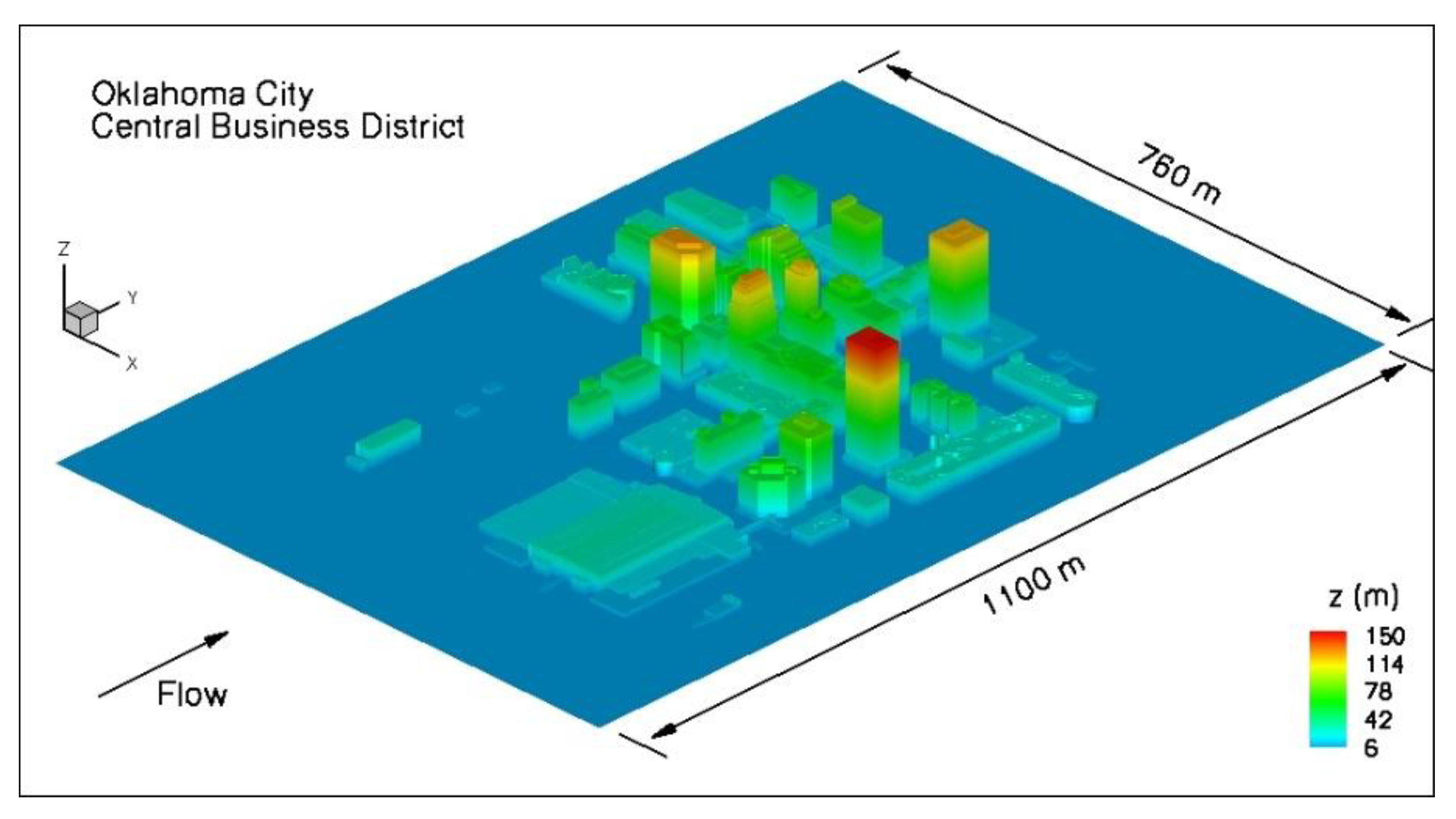
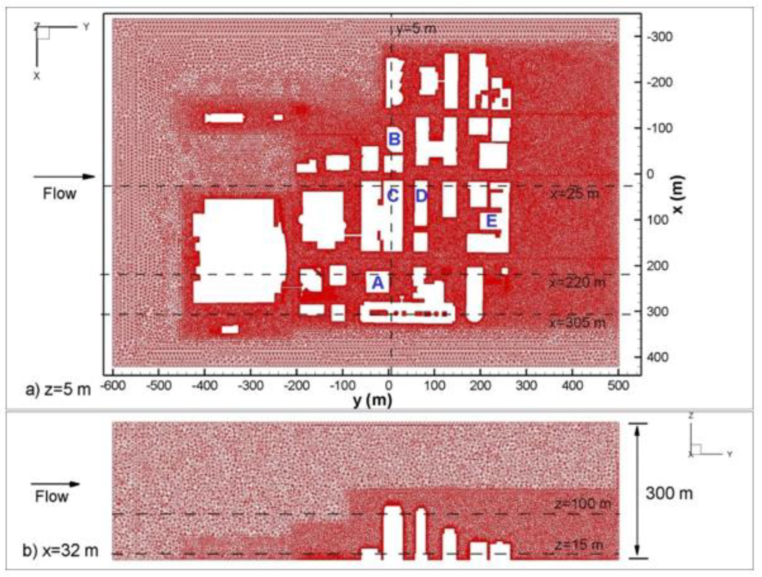
The computational domain used in this study (Figure 1) covers a cluster of buildings in the CBD of Oklahoma City on a neighborhood scale. The average building height is around 50 m (H_a). The tallest building in the domain is 150 m. Following the best practice guidelines for the CFD simulation of flows in the urban environment [25], top of the computational domain is placed at 300 m (6H_a). Lateral boundaries of the computational domain are placed at 100 m (2H_a) to the built area. The distance between the inflow boundary and the built area is 150 m (3H_a). The distance between the outflow boundary and the built area was 250 m (5H_a). This distance was essential to capture physically important flow features in the wake of the building area. A logarithmic velocity profile with 8 m/s average velocity is specified at the inflow section, which was the most commonly tested southerly wind velocity value in the Joint Urban 2003 field campaign. Random fluctuations from a precursor simulation added on the logarithmic profile to generate some turbulence before the building cluster. The turbulent velocity profile is ensured upstream of the first row of buildings. This case also corresponds to the Intensive Observation Period-9 (IOP-9) of the Joint Urban 2003 field campaign. At solid walls, the no-slip boundary conditions are used for the velocities. The hydrodynamic roughness length, z_o, in Equation (1), is chosen as 0.01 m [26]. The free rigid lid boundary condition is assumed on top and lateral boundaries. Constant static pressure is specified at the outlet. The computational domain contained 8.5 million elements. Details of the mesh are shown in a horizontal plane (z = 5 m) and in a vertical plane perpendicular to the streamwise direction (x = 32 m) in Figure 2. Mesh refinement was performed especially in the wake of buildings, to capture physically important scales in the flow (Figure 2). This was achieved by dividing computational mesh into smaller regions. The first point off the wall was located at 1 m, which corresponds to 300 wall units. The time step used in the simulations was 0.025 sec. Results did not change when a higher resolution grid with 10 million elements was tested for grid convergence.

Assuming that the largest eddy will form in the wake of the tallest building (150 m), time series of streamwise velocity is collected inside the separated shear layer from the top of the building. The eddy turnover time for the largest eddy in the domain was found as 10 sec from the power spectrum analysis of this time series. After the fully developed solution is obtained, instantaneous solutions at every 0.2 eddy-turnover time (2 s) were saved over 200 s. to calculate first and second-order statistics. This corresponds to 20 eddy turnover time. The statistics calculated over a longer time span were not so different than the one calculated over 20 eddy turnover time.

Dispersion modeling and the effects of temperature, humidity and other compounds on air density were not considered in the current simulations.

3. Results

The distribution of the buildings has the greatest impact on wind flow patterns. The complexity of the flow field mainly depends on the location of buildings relative to each other and their individual heights.

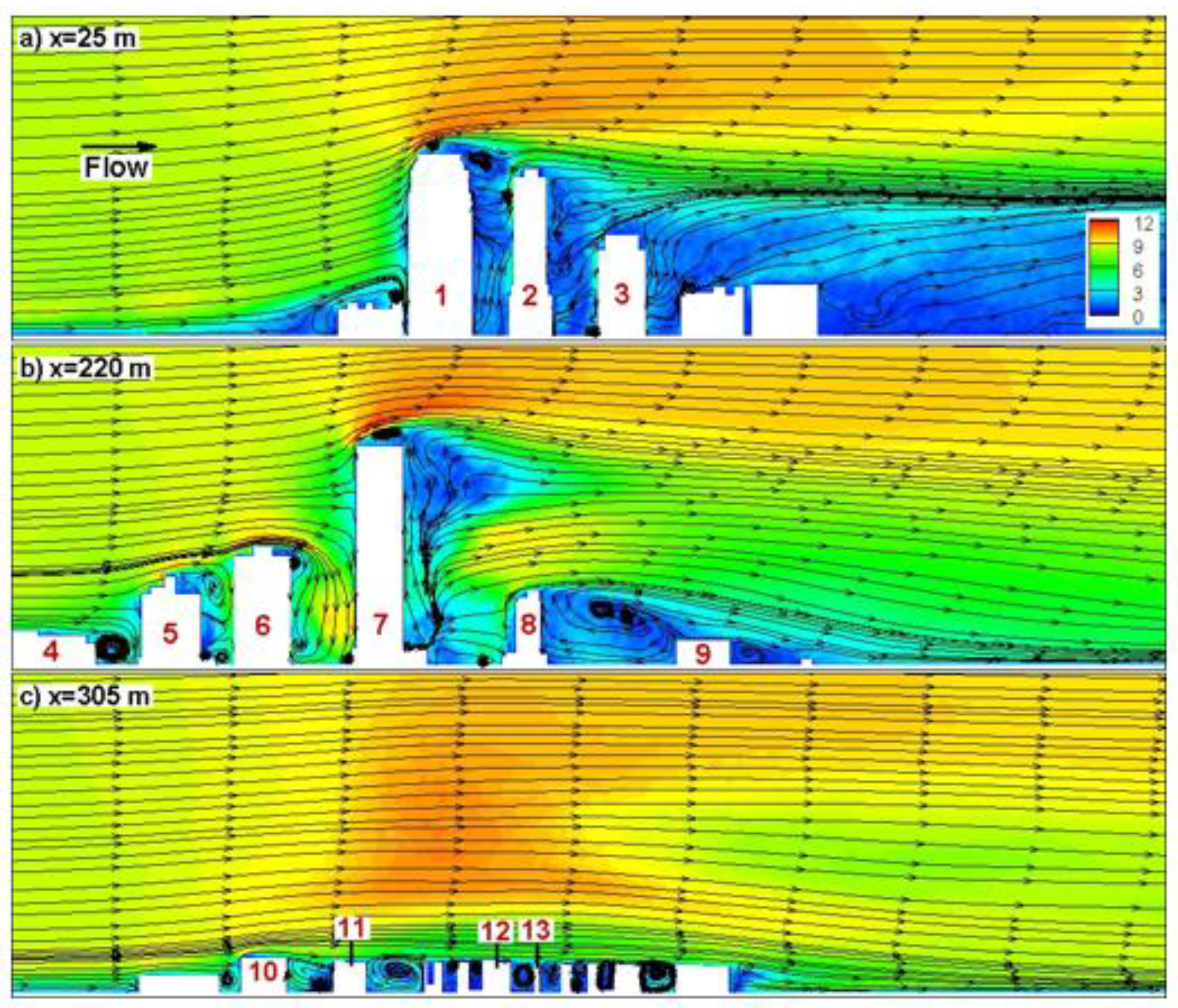
Figure 3 shows the contours of mean velocity magnitude and 2D streamline in x = constant planes. The flow is in the positive y-direction (southerly wind). Three different building configurations are investigated in this figure. In Figure 3a, the buildings are positioned from the taller one to the shorter one in the flow direction. H/D ratios (H is the height, D is the equivalent diameter of the building) for Buildings 1 and 3 are 2.5 and 2, respectively. Stagnation is strongest in the face of building 1. Buildings 2 and 3 are protected from the wind in the wake of Building 1. Since the distances between these three buildings are small, wake regions are not fully developed. A weak updraft is observed between Buildings 1–2 and Buildings 2–3. Figure 3b is an example of reversely sorted buildings (from a shorter one to taller one). H/D ratios for Buildings 5 and 7 are 1.3 and 4.2, respectively. A rear vortex whose axis is in the x-direction is formed in the wake of Buildings 4, 5 and 6. The location of this vortex strongly depends on the height of the building. Since building 4 is the shortest building, the vortex is well developed between Buildings 4 and 5. As building height increases, the axis of this vortex is elevated toward the rear tip of buildings (see Buildings 5, 6 and 7 in Figure 3b). This is consistent with the streamline patterns observed in the wake of single cylinders in [20]. For example, flow around Building 7 (H/D = 4.2) is very similar to the one around the long cylinder (H/D = 10) in [20], where a saddle point forms in the wake of the building.

Another example is the flow around building 5 (H/D = 1.3), which is similar to the one around the short cylinder (H/D = 2.5) in [20], where a strong rear vortex forms in the wake of the cylinder. The rear vortex behind building 5 is weaker compared with [20], due to the existence of building 6, which prevents it from gaining more vorticity and, therefore, more strength. Strong uplift in the wake of Buildings 1, 2, 3 and 7 (chimney effect) was also observed in the simulations of [9]. The rear vortices formed in the wake of Buildings 8 and 9 are similar to the one formed in the wake of building 4. It is also observed that the velocity deficit is stronger in the wake of Buildings 1, 2 and 3 compared with Buildings 4, 5, 6, 7, 8 and 9 (compare Figure 3a,b). Finally, Figure 3c shows a case where the buildings with similar heights (~H/D = 1) are sorted one after another. The flow is like skimming flow over a series of roughness elements [1]. Depending on the distance between buildings, single or multiple cavity vortices are formed. These vortices are commonly named as along-canyon vortices in urban canopy flow studies. The effect of buildings on the outer flow is minimal in this case.

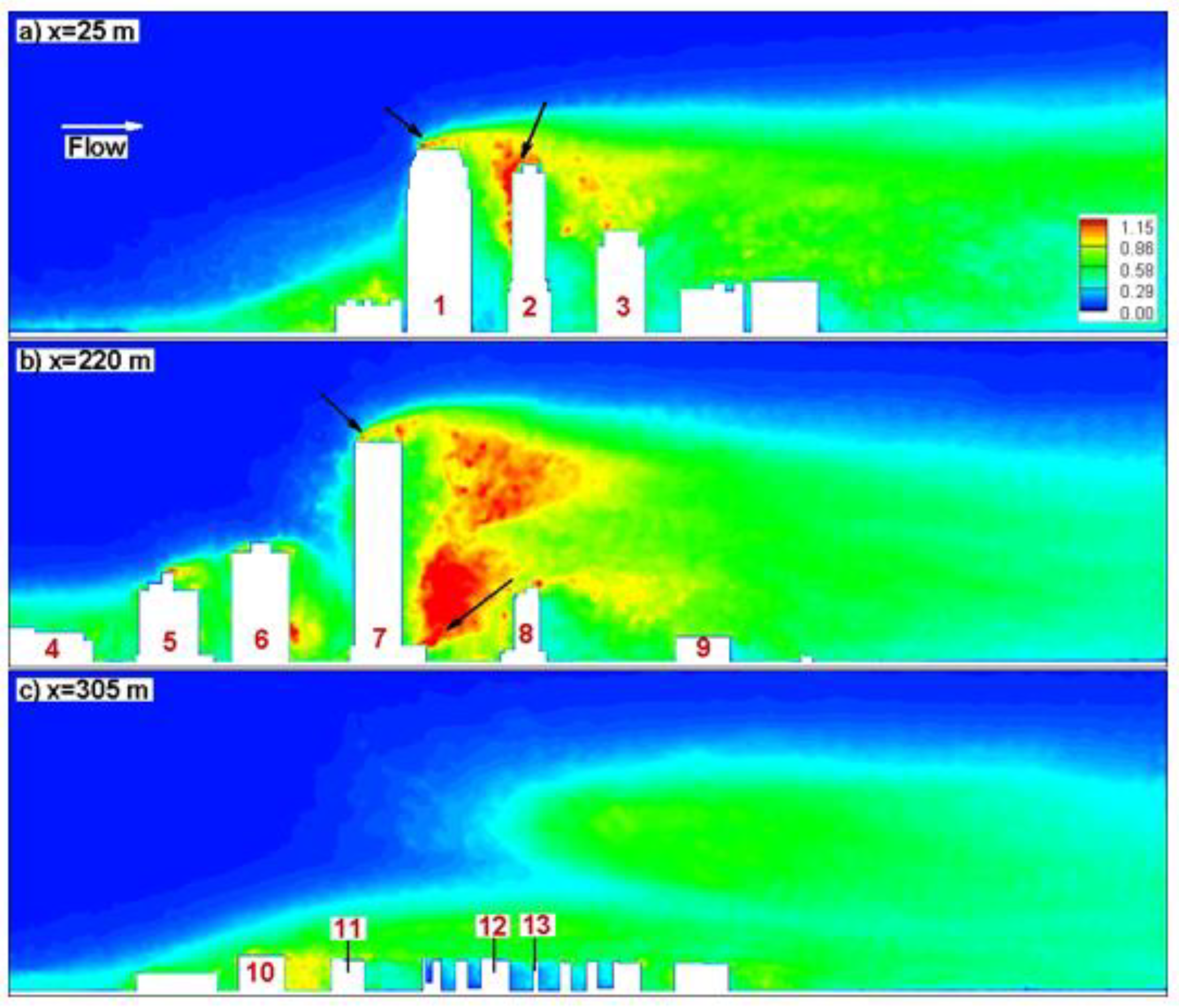
Contours of turbulence intensities are shown in the same x = constant planes in Figure 4. Here, the turbulence intensity is defined as the turbulent kinetic energy normalized by the mean flow kinetic energy. The highest turbulence levels are observed in the separated shear layers at the roof level. The taller building creates a stronger shear layer due to the approaching velocity profile. Strong turbulence generation is observed in the wake of Building 7 because of a strong updraft. Interaction of separated shear layer from Building 1 with Building 2 wall also causes amplification of turbulence (see arrows in Figure 4a). Due to a small distance between Building 1 and Building 2, a strong updraft could not develop. Another observation is that the turbulence intensity amplified between Buildings 10–11, but it is reduced in between Buildings 12–13 (Figure 4c). This is because the distance between Buildings 12–13 is smaller than the one between Buildings 10–11, which prevented any occurrence of the updraft.

As it was stated above, turbulence generation is strongest in the separated shear layers around the buildings. This is more clearly seen in Figure 5, where the turbulence intensities are shown in a plane perpendicular to the flow direction. Separated shear layers around Buildings-B and C are indicated with dashed lines in the figure (Figure 5). Although this plane did not cut through Building A, amplification of turbulence intensity is clear in its wake. Due to the close distance between buildings, the separated shear layers strongly interact with each other, and the region of high turbulence intensity gets wider in the wake of buildings.

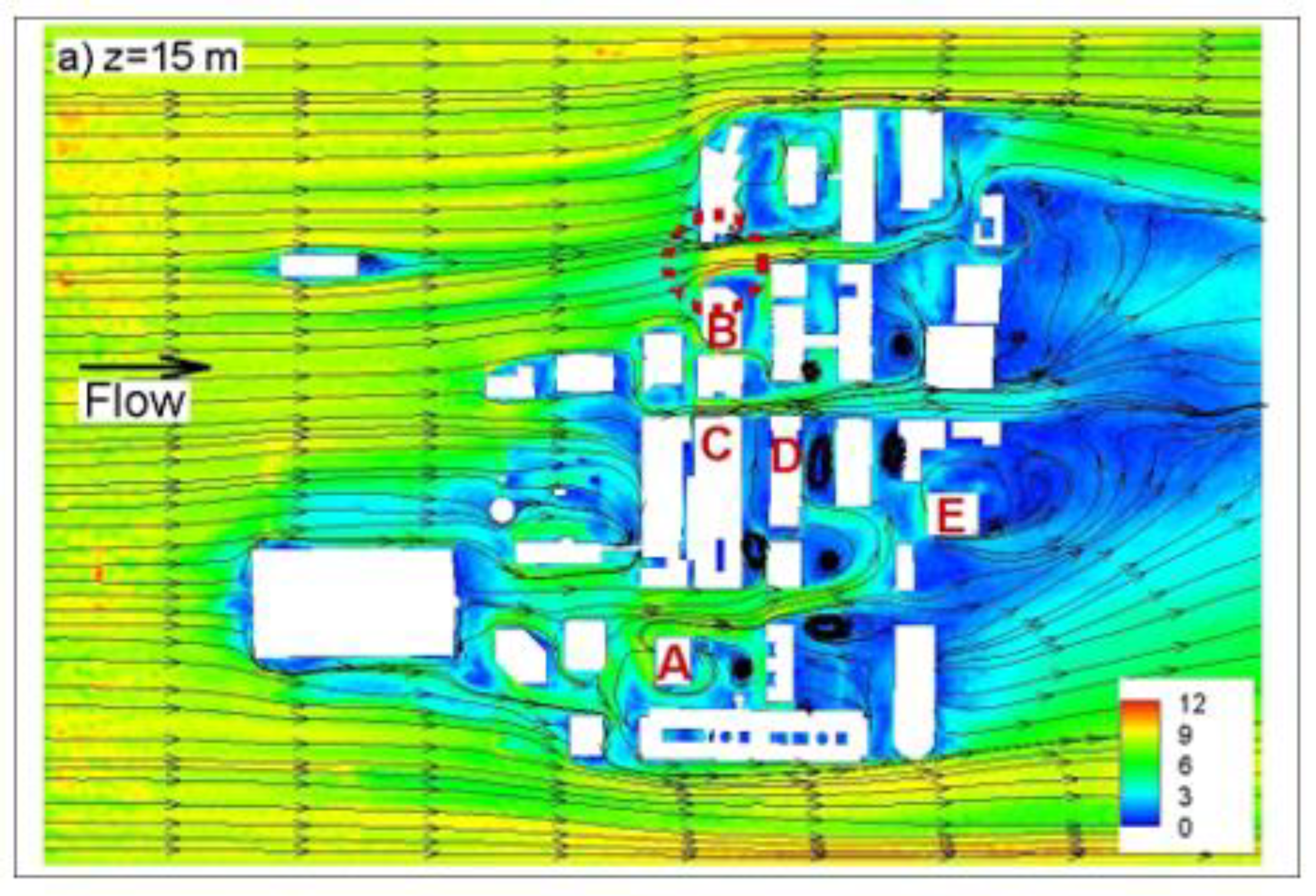
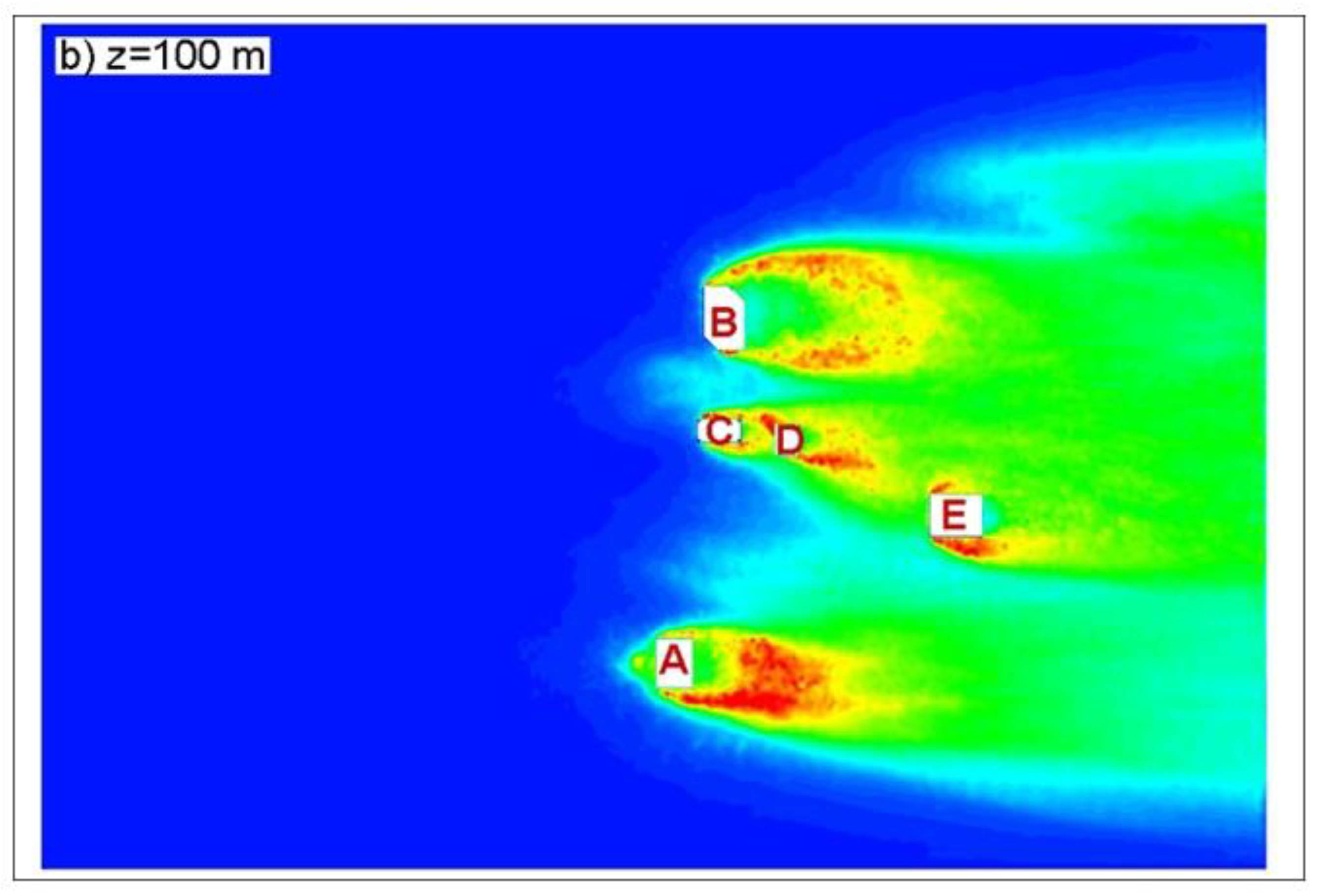
Velocity magnitude contours and 2D streamlines are shown in two horizontal planes in Figure 6. Wind shadows (regions of low velocities) are observed due to blockage of the buildings. Local amplification of velocity magnitude is observed at street level inside the city (see the red dashed circle in Figure 6a). This is mainly because the flow goes through a narrower area due to the high density of the buildings. This is called channeling effect [8]. A similar channeling effect is also observed between Buildings B & C and A & C with a lower intensity, due to flow disturbance caused by low-rise buildings upstream. At this level, highly chaotic flow in time is observed from instantaneous frames. Complex wind patterns are observed as vortices are continuously formed and reshaped (Figure 7). However, at a higher level, z = 100 m (Figure 6b), building density is quite low; this is why double-vortex circulation can be observed in the wake of individual buildings, which is in good agreement with the flow around infinitely long cylinders.

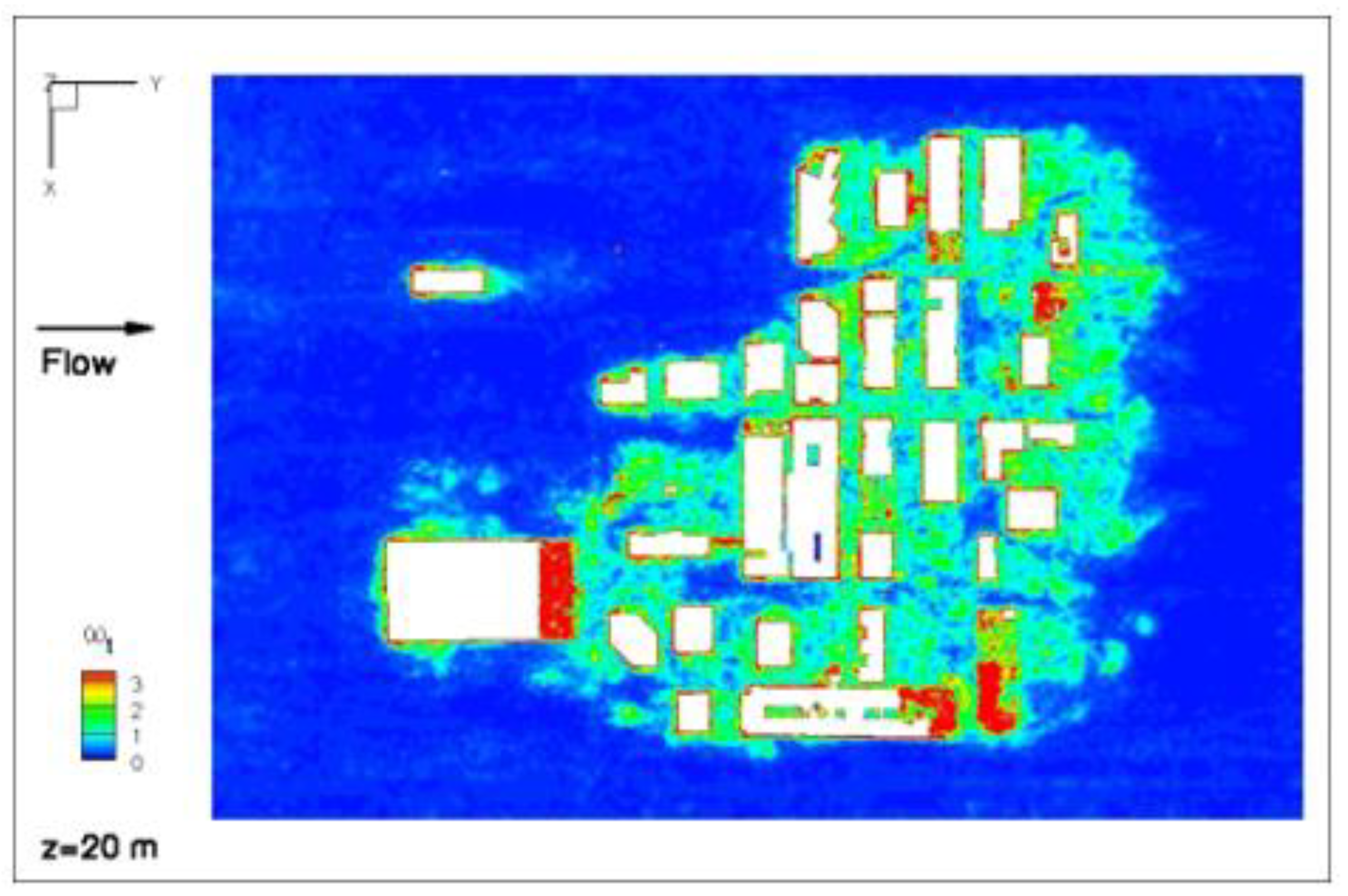
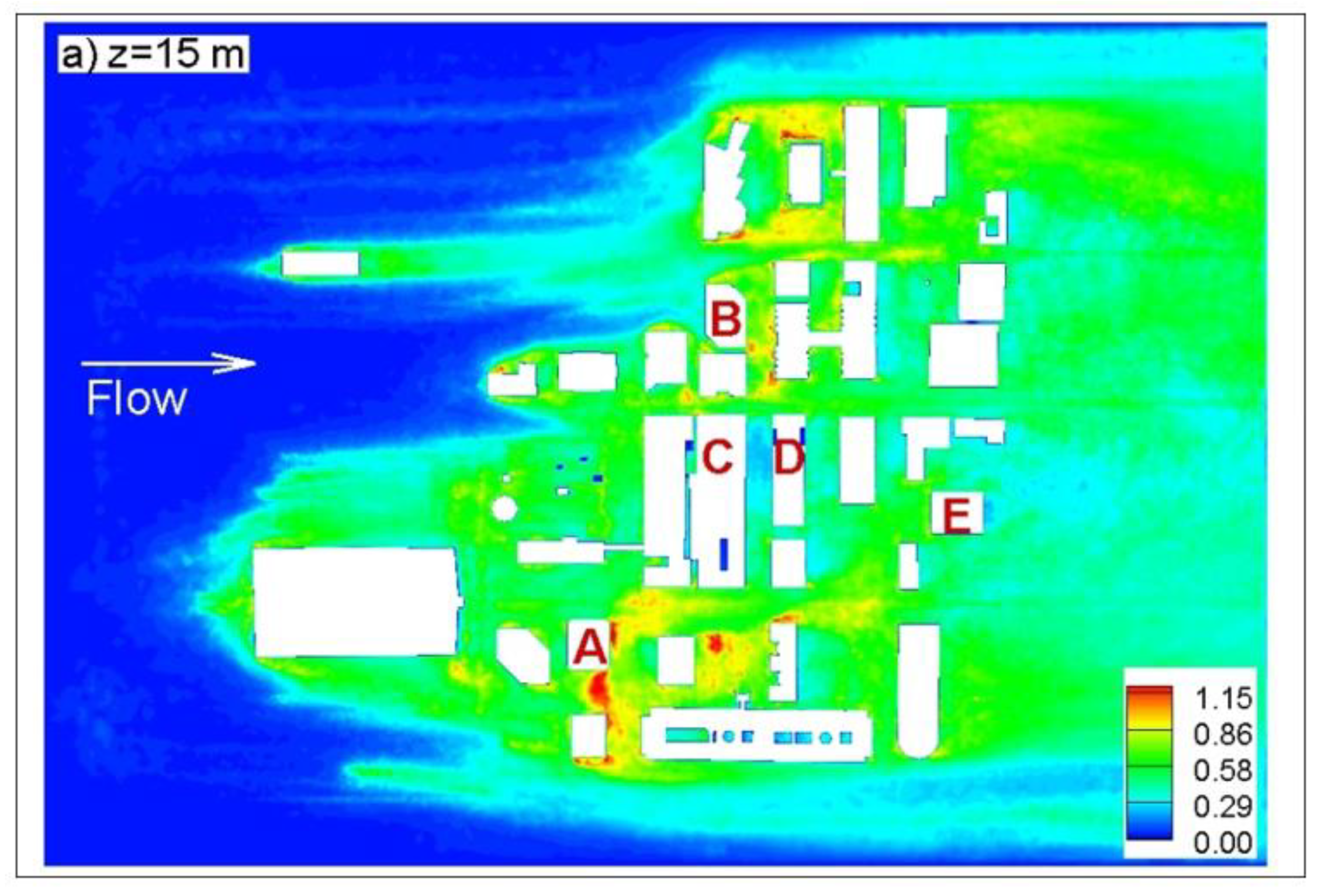
Turbulent intensity contours at the same horizontal planes are shown in Figure 8. Some peak values are observed at the upwind corners of some buildings at street level (Figure 8a), together with a more pronounced boundary layer turbulence. At a higher level (Figure 8b), the turbulence generation is mainly because of separated shear layers. The effect of individual buildings is more pronounced, and wake interference among buildings significantly drops.

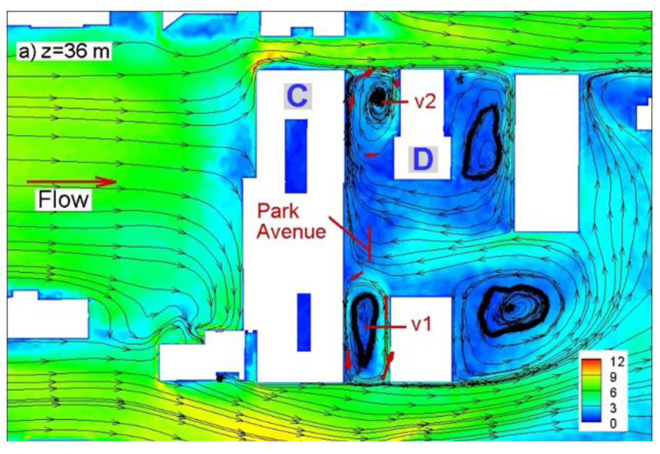
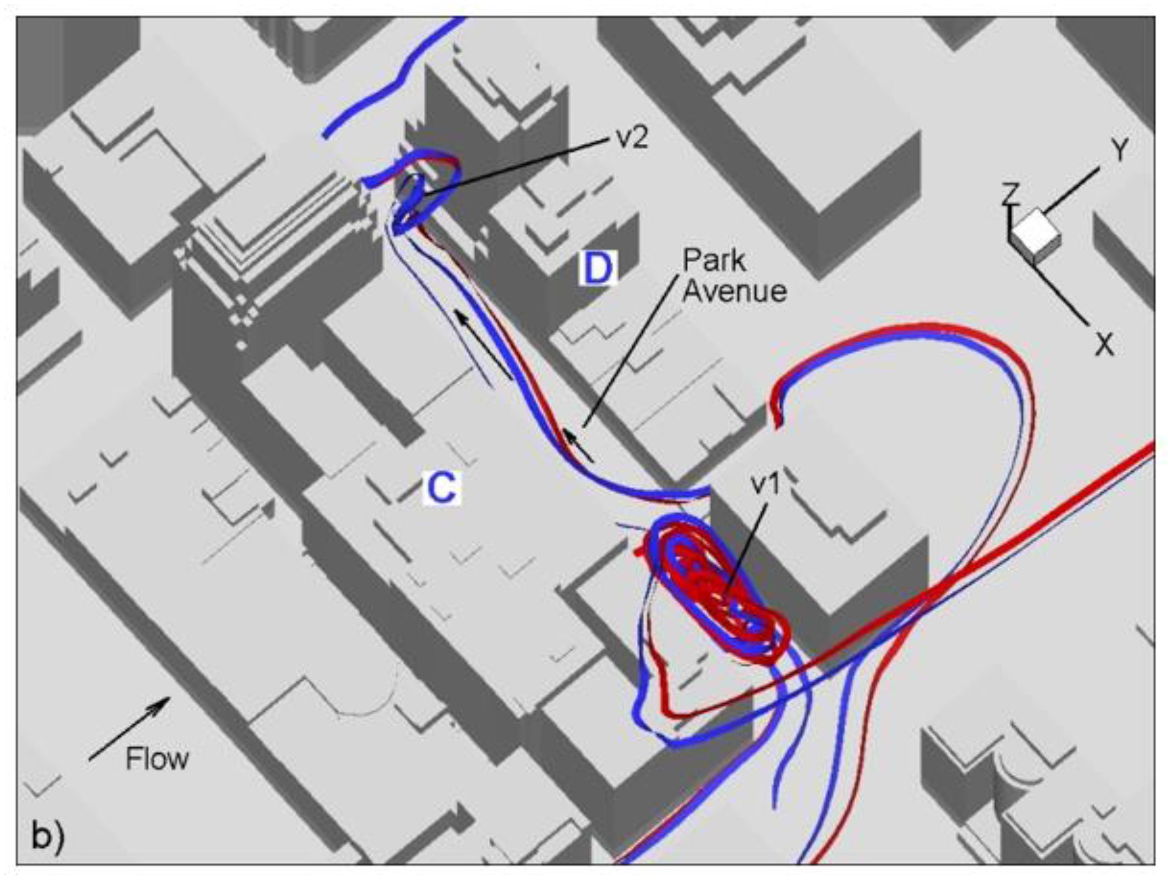
Next, flow structures in Park Avenue, which was densely instrumented during the Joint Urban 2003 experiment are analyzed. Figure 9a shows velocity magnitude contours and 2D streamlines in a horizontal plane near Park Avenue, whereas Figure 9b shows a 3D view of Park Avenue along with 3D streamlines. Westerly channeling together with two end vortices are in very good agreement with observations of [15], and [16]. The corner vortices rotate in opposite directions (Figure 9a). The east corner vortex (v1) is a result of the intermittent injection of momentum from strong southerly wind channeled into the north–south running street next to it (Figure 9b). West corner vortex (v2), on the other hand, is a result of a high–momentum jet coming into the Park Avenue from the north (Figure 9b). This jet first impinges on the south building (building C) and creates westerly channeling towards the west end of the street (Figure 9b). There, the jet creates a strong updraft that rolls into the tornado-like vortex (v2) (Figure 9b). Measured averaged wind vectors (shown as red arrows in Figure 9) during IOP-9 [27], are in good agreement with the result of LES simulation. Consistent with field observations, along-canyon vortex (which is typical to European cities) is not observed along Park Avenue (Figure 9b).

4. Conclusions and Discussions

In this study, a high-resolution LES was used to investigate complex turbulent flow around the buildings located in the Central Business District of Oklahoma City. It was found that the distribution of buildings and their height have the greatest effects on flow patterns. Overall, flow patterns were found to have some similarities with the flow around single submerged cylinders, flow inside cavities and flow over distributed roughness (i.e., ribs). It was found that separated shear layers were the primary reason for turbulence generation in the wake of the buildings. These shear layers strongly interact with each other and cause a wider region to be affected by high turbulence levels. High wind velocities were observed in some regions at the street level due to channeling. Although turbulence generation was due to the boundary layer at lower elevations, it was mainly because of separated shear layers at higher elevations. Strong channeling, updraft–downdraft motions, and end vortices were observed in east–west running streets with heterogeneous building heights when they were subject to southerly winds. East–west running streets were populated with along canyon vortices (cavity vortices) when building heights were homogenous.

LES simulation of wind flows in an urban canopy has the advantage of providing details of 3D complex flow structures around buildings, which are important for heat, contaminant transport and pedestrian comfort in urban areas. The complexity of the flow field mainly depends on the location of buildings relative to each other and their heights. We observed that tall buildings had the greatest impact on wind flow patterns in an urban area. This was due to the fact that separated flow structures in the wake of tall buildings keep their coherence long distances in the streamwise direction and interact with other buildings. Most of the turbulence (therefore mixing) and up and downflows were observed in the wake region of these tall buildings. At lower heights, cavity (or along-canyon) vortices whose axes were perpendicular to the wind direction were observed. In some of the streets, channeling effect in the flow direction cause a significant increase in the mean wind velocity.

The high-resolution LES model was shown to be a useful tool for understanding urban canopy flows. LES has the advantage that the 3D flow field is available everywhere in the domain, which is impossible to obtain during urban field campaigns. Many flow features were resolved successfully, even at the street scale, with the help of a high-resolution computational grid. LES models can be used in similar studies (e.g., other cities, dispersion studies, etc.) in the future.

As a future study, we are planning to solve for contaminant transport equation along with the 3D wind velocity field on the same computational domain. This will give us more detailed information about the urban climate. Another plan is to provide realistic boundary conditions to our LES domain from regional meteorological models.

References

- Britter, R.E.; Hanna, S.R. Flow and Dispersion in Urban Areas. Ann. Rev. Fluid Mech. 2003, 35, 469–496. [Google Scholar] [CrossRef]
- Pullen, J.; Boris, J.P.; Young, T.; Patnaik, G.; Iselin, J. A comparison of contaminant plume statistics from a Gaussian puff and urban CFD model for two large cities. Atmos. Environ. 2005, 39, 1049–1068. [Google Scholar] [CrossRef]
- Calhoun, R.; Gouveia, F.; Shinn, J.; Chan, S.; Stevens, D.; Lee, R.; Leone, J. Flow around a Complex Building: Comparisons between Experiments and a Reynolds-Averaged Navier–Stokes Approach. J. Appl. Meteorol. 2004, 43, 696–710. [Google Scholar] [CrossRef] [Green Version]
- Calhoun, R.; Gouveia, F.; Shinn, J.; Chan, S.; Stevens, D.; Lee, R.; Leone, J. Flow around a Complex Building: Experimental and Large-Eddy Simulation Comparisons. J. Appl. Meteorol. 2005, 44, 571–590. [Google Scholar] [CrossRef] [Green Version]
- Lee, S.-M.; Fernando, H.J.S.; Byun, D.W. CFD Modeling of Fine Scale Flow and Transport in the Houston Metropolitan Area. In Proceedings of the Proc. 5th Symposium on the Urban Environment, Vancouver, BC, Canada, 23–27 August 2004. American Meteorological Society. [Google Scholar]
- Tamura, T.; Nagayama, J.; Ohta, K.; Takemi, T.; Okuda, Y. LES Estimation of Environmental Degredation at the Heat Island due to Densely-Arrayed Tall Buildings. In Proceedings of the Proc. 17th Symposium on Boundary Layers and Turbulence, San Diego, CA, USA, 22–26 May 2006. American Meteorological Society. [Google Scholar]
- Tseng, Y.; Meneveau, C.; Parlange, M. Modeling Flow around Bluff Bodies and Predicting Urban Dispersion Using Large Eddy Simulation. Environ. Sci. Technol. 2006, 40, 2653–2662. [Google Scholar] [CrossRef] [PubMed] [Green Version]
- Zhang, N.; Jiang, W.; Miao, S. A large eddy simulation on the effect of buildings on urban flows. Wind. Struct. Int. J. 2006, 9, 23–35. [Google Scholar] [CrossRef]
- Hanna, S.R.; Brown, M.J.; Camelli, F.E.; Chan, S.T.; Coirier, J.; Hansen, O.R.; Huber, A.H.; Kim, S.; Reynolds, R.M. Detailed Simulations of Atmospheric Flow and Dispersion in Urban Downtown Areas by Computational Fluid Dynamics Models – An Application to Five CFD Models to Manhattan; Report No. UCRL-JRNL-219591; Lawrence Livermore National Lab: Livermore, CA, USA, 2006. [Google Scholar]
- Allwine, K.J.; Flaherty, J.E. Joint Urban 2003: Study Overview and Instrument Locations; Report No. PNNL-15967; Pacific Northwest National Laboratory: Richland, WA, USA, 2006. [Google Scholar]
- Lin, C.-L.; Xia, Q.; Calhoun, R. Retrieval of Urban Boundary Layer Structures from Doppler Lidar Data. Part II: Proper Orthogonal Decomposition. J. Atmos. Sci. 2008, 65, 21–42. [Google Scholar] [CrossRef]
- Flaherty, J.E.; Stock, D.; Lamb, B. Computational Fluid Dynamic Simulations of Plume Dispersion in Urban Oklahoma City. J. Appl. Meteorol. Clim. 2007, 46, 2110–2126. [Google Scholar] [CrossRef]
- Lundquist, J.K.; Chan, S.T. Consequences of Urban Stability Conditions for Computational Fluid Dynamics Simulations of Urban Dispersion. J. Appl. Meteorol. Clim. 2007, 46, 1080–1097. [Google Scholar] [CrossRef] [Green Version]
- Burrows, D.A.; Hendricks, E.A.; Diehl, S.R.; Keith, R. Modeling Turbulent Flow in an Urban Central Business District. J. Appl. Meteorol. Clim. 2007, 46, 2147–2164. [Google Scholar] [CrossRef]
- Brown, M.; Khalsa, H.; Nelson, M.; Boswell, D. Street Canyon Flow Patterns in a Horizontal Plane: Measurements from Joint Urban 2003 Field Experiment. In Proceedings of the Proc. Fifth Symp. on the Urban Environment, Vancouver, BC, Canada, 23–26 August 2004. American Meteor. Soc., CD-ROM, 3.1. [Google Scholar]
- Nelson, M.A.; Pardyjak, E.R.; Klewicki, J.; Pol, S.U.; Brown, M.J. Properties of the Wind Field within the Oklahoma City Park Avenue Street Canyon. Part I: Mean Flow and Turbulence Statistics. J. Appl. Meteorol. Clim. 2007, 46, 2038–2054. [Google Scholar] [CrossRef]
- Hanna, S.R.; Tehranian, S.; Carissimo, B.; Macdonald, R.W.; Lohner, R. Comparisons of model simulations with observations of mean flow and turbulence within simple obstacle arrays Atmospheric Environment. Atmos. Environ. 2002, 36, 5067–5079. [Google Scholar] [CrossRef]
- Xiaomin, X.; Zhen, H.; Jiasong, W. The impact of urban street layout on local atmospheric environment. Build. Environ. 2006, 41, 1352–1363. [Google Scholar] [CrossRef]
- Mou, B.; He, B.-J.; Zhao, D.; Chau, K.-W. Numerical simulation of the effects of building dimensional variation on wind pressure distribution. Eng. Appl. Comput. Fluid Mech. 2017, 11, 293–309. [Google Scholar] [CrossRef]
- Lee, T.; Lin, C.-L.; Friehe, C.A. Large-eddy simulation of air flow around a wall-mounted circular cylinder and a tripod tower. J. Turbul. 2007, 8, N29. [Google Scholar] [CrossRef]
- Vreman, A.W. An eddy-viscosity subgrid-scale model for turbulent shear flow: Algebraic theory and applications. Phys. Fluids 2004, 16, 3670. [Google Scholar] [CrossRef]
- Lin, C.-L.; Tawhai, M.H.; McLennan, G.; A Hoffman, E. Characteristics of the turbulent laryngeal jet and its effect on airflow in the human intra-thoracic airways. Respir. Physiol. Neurobiol. 2007, 157, 295–309. [Google Scholar] [CrossRef] [PubMed] [Green Version]
- Bou-Zeid, E.; Meneveau, C.; Parlange, M. A scale-dependent Lagrangian dynamic model for large eddy simulation of complex turbulent flows. Phys. Fluids 2005, 17, 025105. [Google Scholar] [CrossRef] [Green Version]
- Kappler, M. Experimentelle Untersuchung der Umstro¨ mung von Kreiszylindern mit ausgepra¨gt dreidimen- sionalen Effekten. Ph.D. Thesis, Institute for Hydromechanics, University of Karlsruhe, Kalsruhe, Germany, 2002. [Google Scholar]
- Franke, J.; Hellsten, A.; Schlunzen, H.; Carissimo, B. Best Practice Guideline for the CFD Simulation of Flows in the Urban Environment; COST Action 732 Report; European Science Foundation: Strasbourg, France, 2007. [Google Scholar]
- Stull, R.B. An Introduction to Boundary Layer Meteorology; Kluwer Academic Publishers: Dordrecht, Netherlands, 1998. [Google Scholar]
- Neophytou, M.K.-A.; Gowardhan, A.; Brown, M.J. An inter-comparison of three urban wind models using Oklahoma City Joint Urban 2003 wind field measurements. J. Wind. Eng. Ind. Aerodyn. 2011, 99, 357–368. [Google Scholar] [CrossRef]
Figure 1.
Sketch showing the computational domain: central business district of Oklahoma City.
Figure 2.
Computational mesh (a) in a horizontal plane, z = 5 m; (b) in a vertical plane, x = 32 m. Dashed lines show the location of x- and z- sections used in the analysis.
Figure 3.
2D streamlines and velocity magnitude contours at (a) x = 25 m; (b) x = 220 m; (c) x = 305 m planes (see the location of planes in Figure 2).
Figure 4.
Turbulent intensity contours at (a) x = 25 m; (b) x = 220 m; (c) x = 305 m planes (see the location of planes in Figure 2).
Figure 5.
Turbulent intensity contours at the y = 5 m plane (see the location of the plane in Figure 2).
Figure 6.
2D streamlines and velocity magnitude contours at (a) z = 15 m; (b) z = 100 m planes (see the location of planes in Figure 2).
Figure 7.
Total vorticity magnitude contours at z = 20 m (see the location of planes in Figure 2).
Figure 8.
Turbulent intensity contours at (a) z = 15 m; (b) z = 100 m planes (see the location of planes in Figure 2).
Figure 9.
Flow patterns in Park Avenue; (a) 2D streamlines and velocity magnitude contours; (b) 3D streamlines (see the location of Buildings B and C in Figure 2).
© 2020 by the authors. Licensee MDPI, Basel, Switzerland. This article is an open access article distributed under the terms and conditions of the Creative Commons Attribution (CC BY) license (http://creativecommons.org/licenses/by/4.0/).
Share and Cite
MDPI and ACS Style
Kirkil, G.; Lin, C.-L. Large Eddy Simulation of Wind Flow over A Realistic Urban Area. Computation 2020, 8, 47. https://0-doi-org.brum.beds.ac.uk/10.3390/computation8020047
AMA Style
Kirkil G, Lin C-L. Large Eddy Simulation of Wind Flow over A Realistic Urban Area. Computation. 2020; 8(2):47. https://0-doi-org.brum.beds.ac.uk/10.3390/computation8020047
Chicago/Turabian StyleKirkil, Gokhan, and Ching-Long Lin. 2020. "Large Eddy Simulation of Wind Flow over A Realistic Urban Area" Computation 8, no. 2: 47. https://0-doi-org.brum.beds.ac.uk/10.3390/computation8020047
Note that from the first issue of 2016, this journal uses article numbers instead of page numbers. See further details here.