Simulation of Fire with a Gas Kinetic Scheme on Distributed GPGPU Architectures


Institute for Computational Modeling in Civil Engineering, TU Braunschweig, Pockelsstr. 3, 38106 Braunschweig, Germany
*
Author to whom correspondence should be addressed.
Computation 2020, 8(2), 50; https://0-doi-org.brum.beds.ac.uk/10.3390/computation8020050
Submission received: 24 March 2020
/
Revised: 8 May 2020
/
Accepted: 13 May 2020
/
Published: 26 May 2020
(This article belongs to the Section Computational Engineering)
Abstract
:The simulation of fire is a challenging task due to its occurrence on multiple space-time scales and the non-linear interaction of multiple physical processes. Current state-of-the-art software such as the Fire Dynamics Simulator (FDS) implements most of the required physics, yet a significant drawback of this implementation is its limited scalability on modern massively parallel hardware. The current paper presents a massively parallel implementation of a Gas Kinetic Scheme (GKS) on General Purpose Graphics Processing Units (GPGPUs) as a potential alternative modeling and simulation approach. The implementation is validated for turbulent natural convection against experimental data. Subsequently, it is validated for two simulations of fire plumes, including a small-scale table top setup and a fire on the scale of a few meters. We show that the present GKS achieves comparable accuracy to the results obtained by FDS. Yet, due to the parallel efficiency on dedicated hardware, our GKS implementation delivers a reduction of wall-clock times of more than an order of magnitude. This paper demonstrates the potential of explicit local schemes in massively parallel environments for the simulation of fire.
1. Introduction
Fire is typically associated with a form of combustion that emits sufficient amounts of light and energy to be perceptible and self-sustaining on a macroscopic scale [1]. It has been known to mankind for ages, and for a million years, it has been used for different practical purposes [2]. Still, fire poses a great danger to the lives and well-being of humans. Building fires, such as the Grenfell tower disaster of 2017 in London, U.K., that caused the death of 72 people [3], show that fire safety is an important topic in building design, e.g., [4,5,6]. Fire simulation can be used in multiple ways to improve fire safety especially in the building design phase and in modeling based prediction of catastrophe scenarios. In the example of the Grenfell tower disaster, fire simulation was used a posteriori to investigate the cause of the catastrophe [7]. Other examples of a posteriori fire investigations can be found for example in [8,9,10,11].
The current standard in fire simulation is the Fire Dynamics Simulator (FDS), which is freely accessible and well documented [12,13,14,15]. It is based on a thermal compressible flow solver utilizing a low Mach number approximation. By this approximation, pressure perturbations travel infinitely fast, such that sound waves need not be resolved in the time domain, potentially permitting larger time steps. On the numerical side, this requires the solution of an elliptic pressure equation in every time step. Yet, the elliptic nature of this problem potentially impedes massive parallelization for most solvers available for this problem class. Another CFD code for the simulation of fire is the OpenFOAM [16] extension FireFOAM [17]. In the civil engineering community, also simpler zone models for the prediction of compartment fires are commonly used [18,19]. These models do not resolve the actual flame, but model the time evolution of integral variables in multiple zones and in multiple compartments.
Modern high performance kinetic flow solvers, such as the Lattice Boltzmann Method (LBM) [20,21,22,23], are utilized to compute approximate solutions of the compressible or weakly compressible Navier–Stokes equations. Such explicit schemes tend to require a relatively small time step as compared to implicit methods, but usually require less operations per time step and allow for straight forward parallelization, resulting in near to optimal scaling beyond tens of thousands of compute cores [24,25,26]. A drawback of the LBM is that the full and efficient inclusion of temperature for modeling of thermal compressibility for non-Boussinesq flows is not straight forward. Gas Kinetic Schemes (GKS) are another class of kinetic solvers for computational fluid dynamics. They were originally developed as flow solvers for high Mach number flows with shocks on structured [27,28,29] and unstructured [30,31,32,33] grids with a high order of accuracy [34,35,36,37,38]. GKS for smooth flow fields at low speeds, i.e., without shocks, were investigated in [39,40,41,42,43,44,45,46]. This is the flow regime considered in this work. Additionally, the gas kinetic nature of GKS allows extensions towards rarefied flows and micro fluid dynamics at finite Knudsen numbers in the frameworks of unified GKS [47,48,49,50,51] and discrete unified GKS [52,53,54,55,56,57].
In this work, we present the application of GKS for low speed flows for the simulation of three-dimensional turbulent natural convection and two fire plumes on two different spatial scales under the framework of Large Eddy Simulation (LES). All three tests were validated against experimental data and compared to reference simulations. For high performance computing, massively parallel hardware in the sense of multi-GPGPU was utilized.
2. Gas Kinetic Scheme Solver
In classical fluid mechanics, the flow evolution is described in terms of the Navier–Stokes equations coupled to a continuity and energy equation. This set of non-linear partial differential equations models the conservation of mass, momentum, and energy. Over the last few years, kinetic methods for fluid mechanics gained substantial popularity. Being typically implemented as explicit schemes, such methods show excellent parallel scaling properties. Kinetic methods are based on gas kinetic theory, rather than continuum mechanics. Therein, the fluid state is encoded as a statistical description of (fictitious) particle ensembles. The particle distribution function is the probability to find a particle with velocity at location at time t. Hence, the probability is distributed not only in physical space, but also in velocity space. By considering actual particle motion and interactions, gas kinetic theory covers a more detailed physics than the macroscopic Navier–Stokes equations. The Navier–Stokes equations are in fact a limit of the gas kinetic theory in the case of a very small mean free path, i.e., vanishing Knudsen numbers and for the incompressible case of vanishing Mach numbers. The governing equation in gas kinetics is the Boltzmann equation (here with the Bhatnagar–Gross–Krook (BGK) collision operator [58]):
where is the equilibrium distribution and a relaxation time. Inserting the first-order Chapman–Enskog expansion:
and computing moments in velocity space yield the compressible Navier–Stokes equations.
In order to formulate a numerical scheme for the simulation of macroscopic fluid dynamics, a formal solution of the BGK-Boltzmann equation along particle trajectories is employed [27]. The solution along particle trajectories is approximated by Taylor expansion in space and time, and the initial non-equilibrium distribution is approximated as described in detail in Equation (2). Utilizing the first-order Chapman–Enskog expansion limits the validity of the resulting numerical method to physics described by the Navier–Stokes equations. Fluxes are then computed from the approximated time dependent solution for f.
In the present paper, we consider a simplification for smooth low-Mach number flows of the original GKS [39,45,46]. This simplified scheme has been validated in two dimensions for thermal compressible flows in the setting of natural convection on structured and unstructured grids [45]. Furthermore, a two-dimensional refinement algorithm for quad-tree-type non-uniform Cartesian grids was proposed for efficient grid generation and massively parallel implementation [46]. Therein, the GKS was implemented for GPGPUs utilizing the NVIDIA CUDA frame work [59], and high computational performance was shown. On GPGPUs with thousands of cores accessing the same memory, computational performance is often limited by memory access rather than by floating point operations [60]. The limiting factor in memory access can either be bandwidth or latency. The observation that the two-dimensional GKS utilizes up to 80% of the sustainable bandwidth [46] implies that the GKS algorithm is mostly memory-bound.
The code used in the present paper is a three-dimensional extension of the code used in [46]. The numerical kernel is essentially a straight forward extension to three dimensions, such that the reader is referred to [46] for further details. The same holds for the non-uniform grid implementation, where the procedure from [46] is implemented in three dimensions. The interface ghost cell interpolation coefficients for the second-order accurate interpolation are the same in 3D as in 2D. Additionally, the present code features an explicit sub-grid scale model for LES in terms of a static Smagorinsky eddy viscosity model [61].
A reduced version of the code is available online (with registration) under an open source license [62]. This preliminary version contains no spatial refinement and no combustion model, yet.
3. Performance of the Single GPGPU Implementation
All simulations in this work were run in single precision. The present implementation achieved update rates of up to 300 million cell updates per second for simulation of non-reacting flows on an NVIDIA Tesla P100 GPGPU in single precision. Including the fire module reduced the performance to about 215 million cell updates per second.
The utilization of the hardware for GPGPUs can be measured in terms of bandwidth utilization, because GPGPU computations are often memory limited, i.e., the time to read the data from the memory has a larger effect on the performance than the number of floating point operations. The theoretical peak bandwidth of the NVIDIA Tesla P100 is 732 GB/s. The maximal sustainable bandwidth was measured by the GPU-Stream tool [63]. For the NVIDIA Tesla P100 GPGPUs, the maximal sustainable bandwidth was found to be 543 GB/s. In order to estimate the memory traffic of the algorithm, we counted the number of bytes moved for a single cell update. For non-reacting flow, this was 1041 B. Our code had a net memory traffic of 312 GB/s, which was 57% of the sustainable bandwidth. The actual data traffic was reduced by the utilization of the cache of the GPGPU, which cannot be controlled directly. To gain an estimate, we omitted all computations from the code and performed only read and write operations. With this, we obtained an update rate of 825 GB/s, which was 152% of the sustainable bandwidth. We assumed here that the B B was the actual number of bytes moved for one cell update and that the remaining 356 B were read from the cache. The corrected memory traffic accounted for 206 GB/s, which was 38% of the sustainable bandwidth. An ideal memory bound algorithm would hide all computations with memory traffic. However, for this to be possible, much more threads than cores have to be activated at the same time in the GPGPU. These threads have to allocate their own registers, such that their state persists even though the thread is currently not being processed. This allows for the GPGPU to switch between computation contexts, while threads have to wait for data due to memory latency. This mechanism is called latency hiding. A limiting factor for the number of active threads is the number of registers required per thread. The ratio of the actual number of active threads and the maximum number of active threads supported by the hardware is called occupancy. The occupancy is hence a metric for how well the GPGPU can hide the memory latency. The streaming multi-processors of the P100 support up to 64 warps of 32 threads and provide 65,536 registers. The flux computation kernel in the present GKS required 246 registers. Hence, eight warps could be active at the same time, which resulted in an occupancy of . The actual achieved occupancy for the present implementation was measured with the CUDA profiling tools. The nvprof tool reported a measured occupancy of for the present implementation. This value indicates that latency hiding could not be utilized to its full extent.
4. Multi-GPGPU Implementation
Even though GPGPUs allow high performances for moderate system sizes, their memory is limited. The present paper features multi-GPGPU communication to overcome this limitation. The GKS algorithm is comprised of only local support, i.e., the flux computation requires only the next neighbor information. For multi-GPGPU, the flow domain is split into box-shaped sub-domains, where each sub-domain is processed by one GPGPU. For complete communication, it is sufficient to exchange a single layer of cells between neighboring sub-domains. The last layer of cells in the sub-domain is sent to the neighboring process, and one layer of communication ghost cells outside the sub-domain is received from the same neighboring process.
The communication procedure is shown in Figure 1. The flow state data of the exchanged cells is not continuous in memory. Therefore, as a first step, the flow state data of the sending cells is collected in a send buffer by a kernel. This send buffer is then sent to the neighboring process via Message Passing Interface (MPI) library calls. There, the data are received in a receive buffer and subsequently distributed to the communication ghost cells. These ghost cells are located at the same location as the corresponding send cells in the physical space of the simulation domain, but are directly outside the receiving sub-domain. Furthermore, the send and receive buffers must be downloaded and uploaded, respectively, because MPI can only access host memory. The host is the computer containing the GPGPU. Some modern MPI implementations feature CUDA support, where the network adapter can directly access GPGPU memory to improve communication performance. This procedure was implemented, but not used for the results in this work.
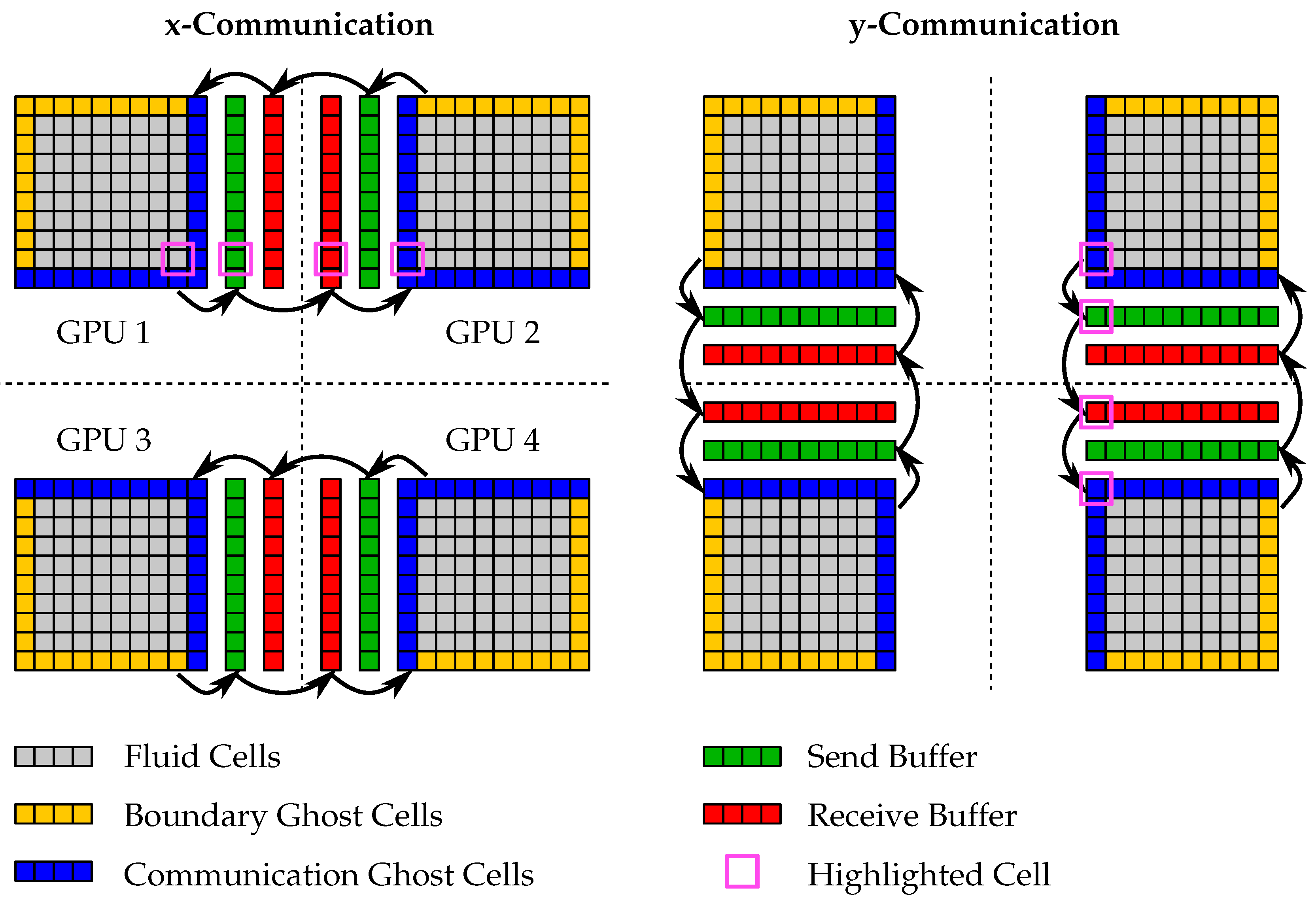
In three dimensions, one sub-domain can have a total of 26 neighboring sub-domains, connected via faces (6), edges (12), and corners (8). In order to reduce the number of communication neighbors, sequential communication along the coordinate axes is used; see Figure 1. This effectively reduces the number of communication neighbors to the six face neighbors. Sequential communication means that all communication in x-direction is completed on one process, before communication in the y-direction is started on this process. Similarly, the z-communication must only start after the y-communication is finished. In this way, information is also passed over edges and corners; see the highlighted cell in Figure 1.
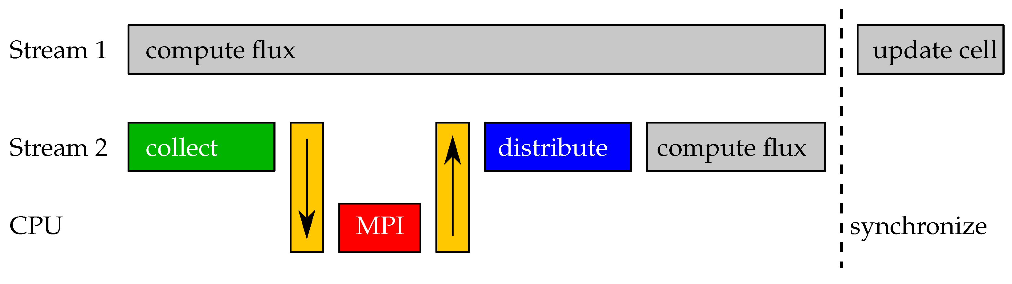
Communication is a severe bottleneck in distributed computations. For GPGPUs, this effect is not as prominent as for distributed CPU communications, because the problem size per sub-domain is usually large compared to the message length of the communication. Nevertheless, communication invokes performance losses. The CUDA framework offers remedies for this. On CUDA-enabled GPGPUs, the compute hardware and the memory management hardware are mostly independent. The compute hardware can process data while memory is transferred between GPGPU and host memory. Further, compute kernel invocations are non-blocking with respect to the host, such that the host side communication (invocation of MPI routines) can also be done while the GPGPU processes data. This allows for communication hiding, which aims at performing computation and communication concurrently. Communication hiding is state-of-the-art in distributed GPU computing. Examples for communication hiding in LBM can be found, e.g., in [64,65,66].
The flux computation on cell faces in the vicinity of the sub-domain boundaries depends on the received cells. In order to keep the code logically consistent, the set of cell faces is divided into two sub-sets. The first contains all cell faces that were independent of the communication and the second faces that depend on the communication. The second set can only be processed after the communication is complete. Communication hiding is implemented in terms of CUDA streams. CUDA streams are independent queues, where each queue processes its tasks sequentially. One stream is used for the evaluation of the first sub-set of cell faces; see Stream 1 in Figure 2. This kernel is invoked first. The second stream handles all communication and interacts with the CPU; see Stream 2 in Figure 2. It finally computes the fluxes of the second sub-set of cell faces. The independent execution of the two streams is synchronized after the flux computation, and finally, all cells are updated. Figure 2 accounts for a single time step with communication in only one direction.
The algorithm for a single time step with communication hiding is given in Algorithm 1. This algorithm is an extension of the nested time stepping algorithm for GKS on a single GPU published in [46]. We utilize recursive time stepping to implement the nested time steps. The time step function is called with a level and a time step length. Each time step starts with the fine to coarse interpolation, if the current level is not the finest one. Subsequently, boundary ghost cells are set to fulfill the boundary conditions. Then, all faces that do not depend on communication on this level are processed. This is invoked in a non-blocking manner on the compute stream (Stream 1). Concurrently, the communication is performed on the communication stream (Stream 2). Here, we see the sequential communication per coordinate direction. When the communication is finished, the remaining faces are processed also on the communication stream (Stream 2). Afterwards, the streams are joined, by synchronizing the device, i.e., waiting for all streams to finish. If this level is not the finest, the coarse to fine interpolation is performed, and the nested time step function itself is called twice for the next finer level with half the time step length. This is the essence of nested time stepping. Performing two shorter time steps on the finer level saves time step evaluations on coarser levels by satisfying a local stability criterion instead of a global one. At the end of each time step, the cells are updated, i.e., the fluxes that were collected in an update variable are added to the current flow state. This function is repeated for the length of the simulation.
| Algorithm 1 Recursive nested time stepping for multi-GPU. |
|
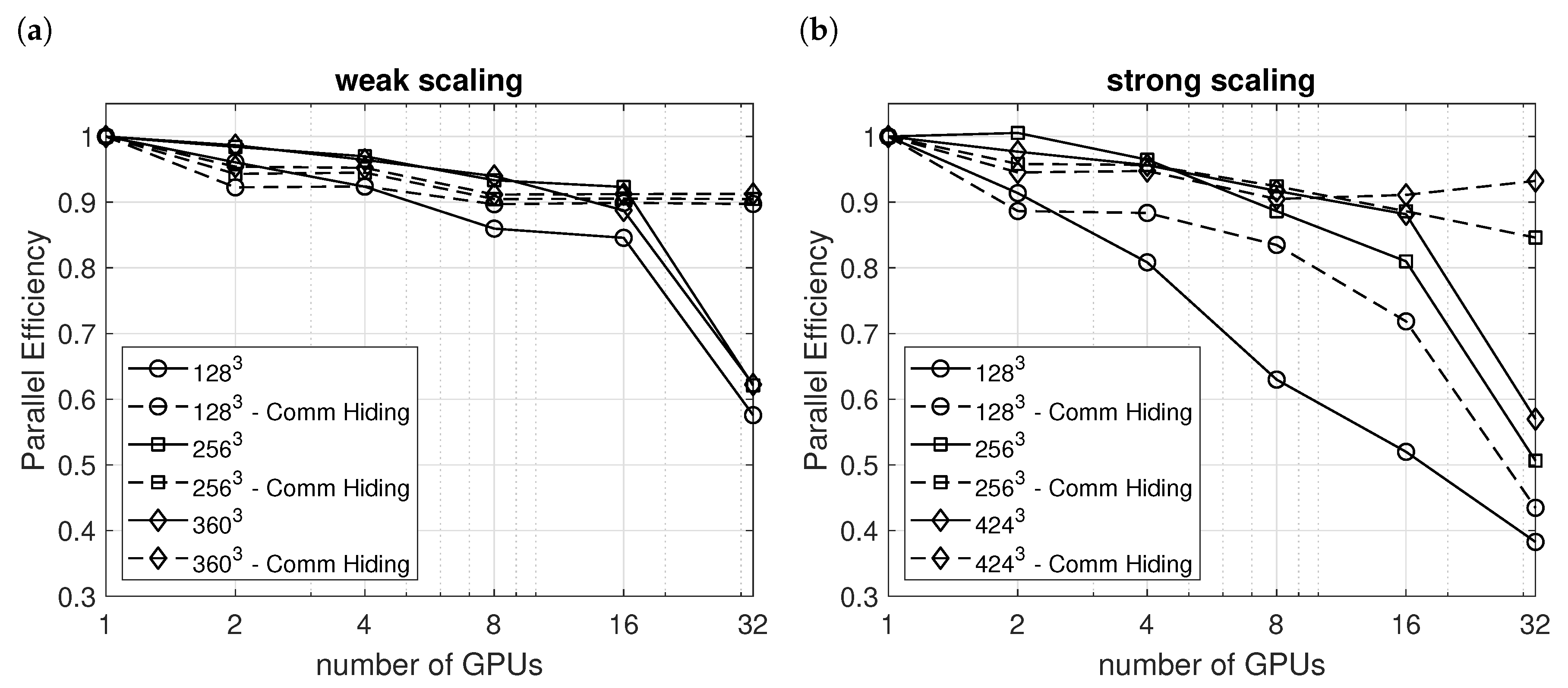
The performance of the multi-GPGPU implementation was measured in terms of parallel efficiency. The parallel efficiency is the ratio of the run times of coupled and independent sub-domains, i.e., with and without communication. The scaling was observed from a single GPGPU (as baseline) up to 32 GPGPUs. The baseline grid was a cube with uniform resolution. Under weak scaling, the workload per GPGPU is kept constant, such that the base cube was multiplied by the number of GPGPUs. Under strong scaling, the total workload is kept constant, such that the base cube was split into as many parts as there were GPGPUs. The decomposition with two GPGPUs was one-dimensional (), with four GPGPUs two-dimensional (), and with eight and more GPGPUs three-dimensional (, , and ). All tests were performed on the PHOENIX (https://www.tu-braunschweig.de/en/it/dienste/21/phoenix) compute cluster at TU Braunschweig, Germany. The cluster provides eight GPU nodes. Each is equipped with two INTEL Xeon E5-2640v4 CPUs, 64 GB of RAM, and four NVIDIA Tesla P100 GPUs with 16 GB HBM2 memory each. The nodes are connected by an Intel Omni-Path high speed network.
For weak scaling, the communication hiding was able to keep the parallel efficiency above for all tested problem sizes; see Figure 3a. Without communication hiding, the performance deteriorated at 32 GPGPUs, which was related to the hierarchical network topology in the HPC-system utilized for these benchmarks. The first 20 GPGPUs were connected to the same switch, while the remaining 12 GPGPUs were connected to another switch, such that the communication had to go an additional step. The good performance under weak scaling was due to the constant favorable ratio of computation per communication. For strong scaling, this ratio successively deteriorated, which can be seen in Figure 3b. For the larger problems, the communication hiding was able to keep the efficiency above . For the smallest problem size, parallel efficiency deteriorated also when communication hiding was utilized. This was due to the small number of cells () per GPGPU, such that the GPGPUs could not utilize their full potential due to reduced latency hiding.
This section shows that the present implementation can efficiently distribute the workload to multiple GPGPUs, given that the total problem size is large enough.
5. Combustion Model
The GKS flow solver is augmented with a simple combustion model to demonstrate its applicability to simulate fire. The basic GKS tracks a single component fluid. For the simulation of fire, the local composition of this fluid is required. In GKS, multiple components can be implemented by tracking partial densities [67]. As an alternative, the single density can be split into multiple components based on transported scalars. In this paper, we follow the second approach. We use the scalar transport scheme for GKS proposed by Li et al. [68].
The fluid in the present model is composed of the three components, fresh air, gaseous fuel, and combustion products with mass fractions , , and , respectively. The two mass fractions of fuel and products are tracked explicitly in the simulation as scalar quantities, and the mass fraction of air is given implicitly by requiring that the sum of mass fractions is one. These three components are a simplification of the five species actually present in the reaction under consideration. Fresh air is comprised of a fixed mixture of oxygen, , and nitrogen, . The fuel is assumed to be pure methane, . The reaction products are a fixed mixture of carbon dioxide, , water, , and nitrogen, . The nitrogen is assumed to be inert. The stoichiometry of the one-step reaction is described by:
where all chemical symbols are to be interpreted as one of the species and is a stoichiometric factor of nitrogen that passively accompanies the reaction. The combustion of methane is an exothermic reaction with the molar heat of combustion . In reduced species, the reaction is:
where , , and are the mole fractions of air, fuel, and products, respectively, and denotes that only parts of the present amounts react. For the conversion of mole and mass fractions, see Appendix A. The reaction can similarly be written in terms of mass fractions with being the mass specific heat of combustion, such that:
From the stoichiometry in the full reaction Equation (3), we see that . In terms of mass fractions, the exact reaction mixture is given by the ratio:
where denotes molar masses. Finally, the reacting mass of fuel is defined by the minimum amount of fuel and oxygen as:
The mass of oxygen is computed from the mass of air by:
where is the mole fraction of oxygen in fresh air.
In more advanced models, the rate of the reaction is given by an Arrhenius-type reaction rate. In LES simulations such as discussed in this work, the reaction time scale is much shorter than a time step of the flow solver. In addition, a reaction can only take place where both fresh air and fuel are present, i.e., where they are mixed. Real mixing can only happen by molecular diffusion, which is usually slow. Turbulence can increase the diffusion by increasing the gradients and contact areas of the diffusing species. In LES, the small-scale turbulence is not resolved. Hence, the reaction is mixing limited, because reaction is fast and mixing is slow. In order to capture this behavior and the influence of the turbulence on the combustion, a model similar to the default model of Version 5 of FDS [69] is implemented.
The task of the combustion model is to predict the mass of reacting fuel . For this, the “mixed is burned” assumption is used [13]. In LES, the flow structures are usually not fully resolved, such that the flame-air interface thickness is much smaller than the cell size. Hence, a cell in the vicinity of the flame front will contain fuel, air, reacting fuel air mixture, and products. In this way, cells can be partially mixed. Thus, the assumption of instantaneous reaction in the mixed part of the cell is justified and adopted. The mixing time scale in the FDS 5 combustion model [69] used here is:
where is the eddy diffusivity predicted by the sub-grid scale turbulence model. The mixed fraction of a cell is , where is the time step of the flow simulation. The local heat release rate is then given by:
The amounts of consumed fuel, oxygen, and air over one time step are:
and
respectively. Finally, the updates of mass fractions and energy due to the reaction are implemented as:
Including this reactive model into the GKS solver induced additional stability issues. Accordingly, suitable limiters are designed to stabilize the simulations. At the leading fronts of flame plumes, excessive temperatures are observed. Thus, thermal diffusivity is locally increased in the presence of large temperature gradients as:
where is the increased thermal diffusivity, is an upper bound, and is an adjustable constant. This limiter smears out severe temperature peaks.
The scalar transport equations are subject to dispersion errors that produce negative and excessive mass fractions. Increased diffusivities are again used to repair this defects in a conservative fashion. The increased diffusivity for the generic passive scalar is:
where is an adjustable constant. In this work, is chosen for all simulations.
Finally, the maximal local heat release is limited by an upper bound, i.e.:
where is the limited heat release rate and a maximal allowed heat release rate. Such a limiter is also used in Version 5 of FDS [69].
6. Validation
This section features three validation cases for the present flow solver. First, a simple setup of turbulent natural convection at a high Rayleigh number was simulated and compared to experimental data. Then, a small-scale and a large-scale fire were simulated and compared to experimental data to validate the combustion model. These results were also compared to the results obtained with Version 6 of FDS.
6.1. Turbulent Natural Convection
In our prior work on the development of GKS, we extensively validated GKS in two dimensions for various natural convection-related simulations, featuring validation based on reference simulations [45,46]. These included simulations of moderate Rayleigh numbers at high temperature differences and high Rayleigh numbers at small temperature differences due to the limited availability of reference data. In the present study, we present three-dimensional validation against experimental data. The availability of experimental data is, to the best of our knowledge, scarce. Ideally, we would seek a reference with a large temperature difference and a high Rayleigh number. The setup we feature here was investigated experimentally by Tian and Karayiannis [70,71] and numerically by Salinas-Vázquez et al. [72]. The setup includes a target Raleigh number of:
and a dimensionless temperature difference of:
where is the mean temperature. These parameters can be qualified as a high Rayleigh number, but at a small temperature difference compared to the we used in the previous two-dimensional tests [45,46].
The experiment was performed in a square cavity with dimensions = 0.75 × 1.5 × 0.75 [70]. The x-normal walls were kept at hot and cold temperatures, respectively. In the experiment, the wall temperatures were and . Top and bottom walls, normal to the z-axis, were highly conducting, such that the experiment produced non-uniform temperature profiles along these walls. This is contrary to synthetic cavity flows with differentially heated sides, such as the benchmarks by de Vahl Davis [73] and Vierendeels et al. [74], where top and bottom walls were not insulated. In the simulations, a cubic fit of the measured data in the experiment was used. The fitted profiles are:
and
with for top and bottom temperatures and , respectively.
Further parameters for the simulation were a barometric number of (see [45] for the definition), a Prandtl number , and internal degrees of freedom for the fluid molecules. The barometric number was set by the reference temperature and the Rayleigh number by viscosity. All remaining parameters were chosen as unity. The temperature dependent viscosity was modeled by Sutherland’s law; see, e.g., [75]. All velocity related results were normalized by a reference velocity [70]:
The gravitational acceleration g is implemented based on the so-called well-balanced scheme of Tian et al. [76].
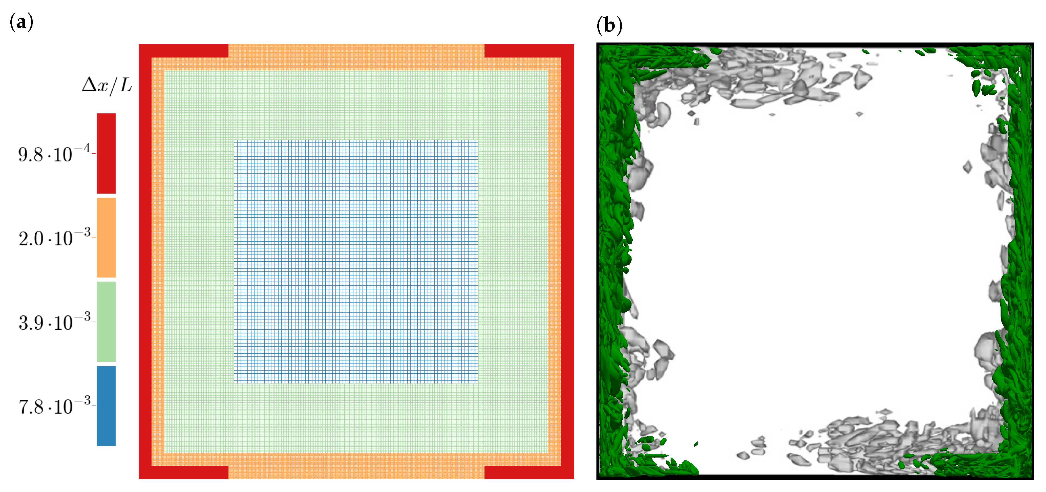
The flow domain for the present simulation was a cube with dimension and with periodic boundary conditions in the y-direction to resemble the larger extent of the experimental cavity. The flow domain was discretized by a non-uniform grid with four grid levels and refinement towards the walls; see Figure 4a. The background grid had a resolution of such that the third refinement level had a wall resolution of . This wall resolution was slightly coarser than the wall normal resolution in the reference simulation of Salinas-Vázquez et al. [72] where a stretched grid with at the wall was used. The grid was distributed to eight GPGPUs with a layout of subdomains.
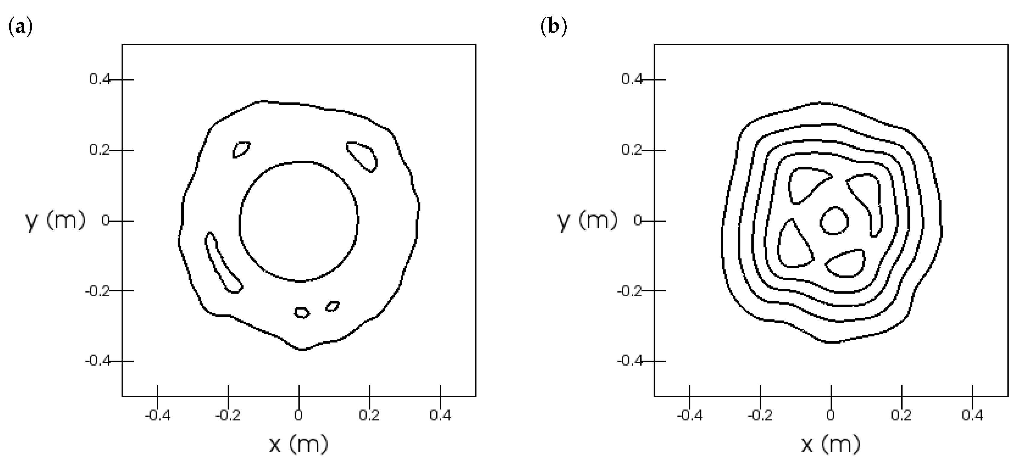
As a first result, we show instantaneous turbulent structures as iso-surfaces of the Q-criterion [77]. It is apparent that the present simulation and the results of Salinas-Vázquez et al. [72] did not match in detail as the latter showed increased levels of turbulence on top and bottom walls.
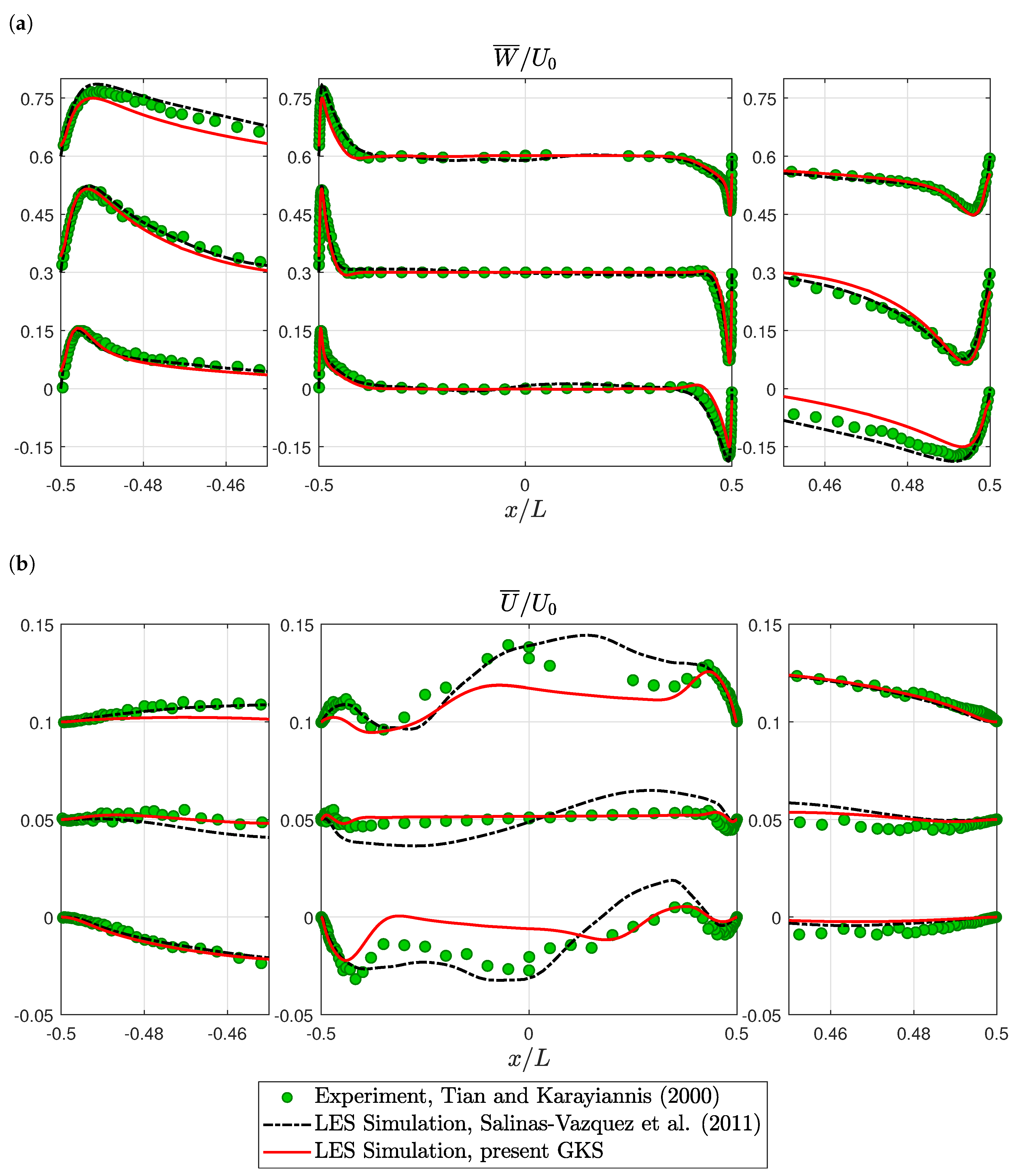
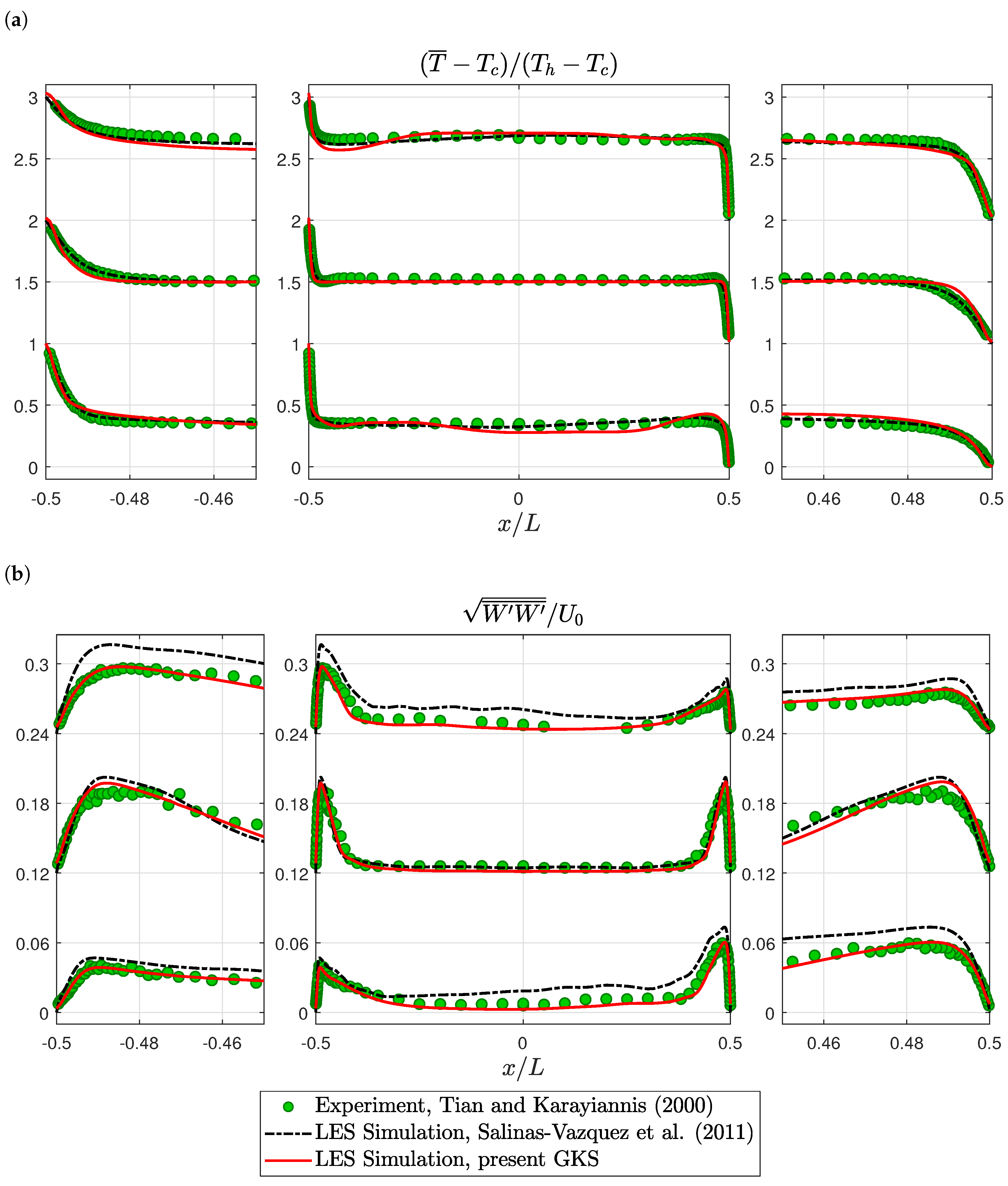
For a more detailed validation, time averaged velocity profiles are compared. Vertical velocity profiles matched the experimental data well; see Figure 5a. The GKS slightly under-predicted the peak velocities on the top left and bottom right, while the reference simulation over-estimated these velocities. The horizontal velocities showed large discrepancies between all three datasets, such that no clear result could be gained; see Figure 5b. In the temperature profiles, the present GKS results showed deviations from the experimental data that were not present in the reference simulations; see Figure 6a. The GKS results were non-monotonic, i.e., they under-estimated temperature just outside the heated boundary layer and over-estimated temperature just outside the cooled boundary layer. Overall, the temperature field was captured well. The thermal boundary layer thicknesses were correctly estimated. Finally, the turbulence was measured as the root-mean-squared vertical velocity fluctuation. The reference simulation substantially over-estimated the turbulence on top left and bottom right, while the GKS essentially correctly predicted the strength and profile of the turbulence; see Figure 6b. This finding is consistent with the discrepancy in turbulent structures, observed in Figure 4b. It supports the interpretation that the present GKS results resembled the experiment better in that region than the reference simulation.
Overall, this simulation validates the usage of the present GKS for convection-driven turbulence.
6.2. Purdue Flame
The reference software for fire simulation FDS in its current Version 6 [12] has been validated for hundreds of test cases; see [15]. Two of these test cases are considered here. The first example is a table top experiment performed at Purdue University, USA, and published by Xin et al. [78]. The experiment featured a methane flame over a cm diffuser burner with an outlet velocity of , a mass flow rate of , and hence, a density of . With the specific heat of combustion for methane of , the total heat release rate of the flame is given by .
This setup was computed with both FDS Version 6 and with the present GKS. The FDS input file for this test case is available in the FDS repository on GitHub [79]. The computational domain for GKS spaned with uniform spatial resolutions of cm and cm for a coarse and fine simulation, respectively. The lateral sides of the domain featured an open boundary condition that allowed inflow at ambient conditions if the internal pressure is below the ambient pressure and prohibits outflow. The top of the domain was a pressure outflow boundary that explicitly prohibits inflow. The bottom was an insulated wall, and the burner was modeled as a Neumann boundary for mass flux and a symmetry boundary for velocity and temperature.
The simulation was performed at physical parameters with density of air , gravitational acceleration , viscosity , , and . In order to accelerate the simulation, ambient temperature and heat of combustion were scaled down by a factor of 100. This substantially increased the Mach number and reduced the discrepancy between the time scales of the hydrodynamic and the acoustic modes.
The gravitational acceleration was implemented in a different way than in the previous example for these fire simulations. The acceleration only changed momentum in the cell while temperature was kept constant. The energy was then computed from the new momentum and the old temperature. The temperature and heat release rate limiters were effectively turned off for this test case by setting a low value for and a very large value for .
In this work, we aim at comparing two completely different numerical methods and implementations, which are, to a certain degree, able to simulate similar physical setups. The main difference between the present GKS and FDS is the basic flow solver. Apart from that, the present GKS utilizes a static Smagorinsky turbulence model, while FDS implementes a local version of Deardorff’s turbulence model [13,80]. Further, the present GKS employes a simple combustion model with a single reaction time scale that modeles the turbulent mixing. In FDS, this model is refined by taking into account multiple physical mixing processes that play a role in the computation of the mixing time scale. Therein, mixing on coarse scales is based on buoyant mixing, while the turbulent mixing time scale comes into play at intermediate scales. On small scales, diffusive mixing is modeled. Hence, this refined model takes into account the mixing mechanism present on the scale of the grid cells.
A detailed comparison between FDS and GKS was not possible because many aspects are implemented differently. Hence, we aim at a comparison of the final results, only. These are compiled as time averaged profiles of flow properties in addition to the absolute wall-clock time required for the simulation. The quality of these results can be assessed independently of how they were produced. This comparison does not give any insight into which part of the software triggered certain deviations between the results of both simulations, though.
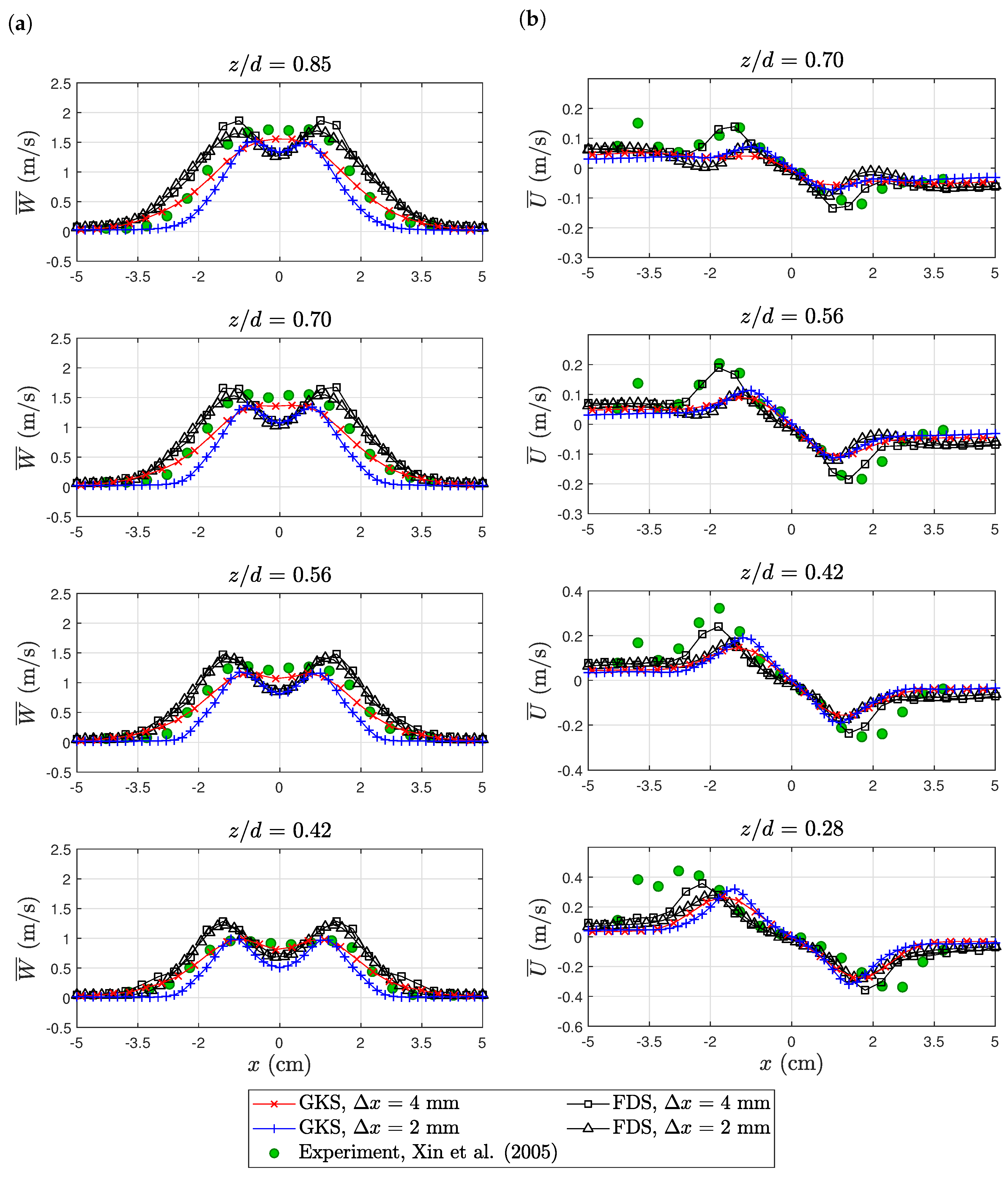
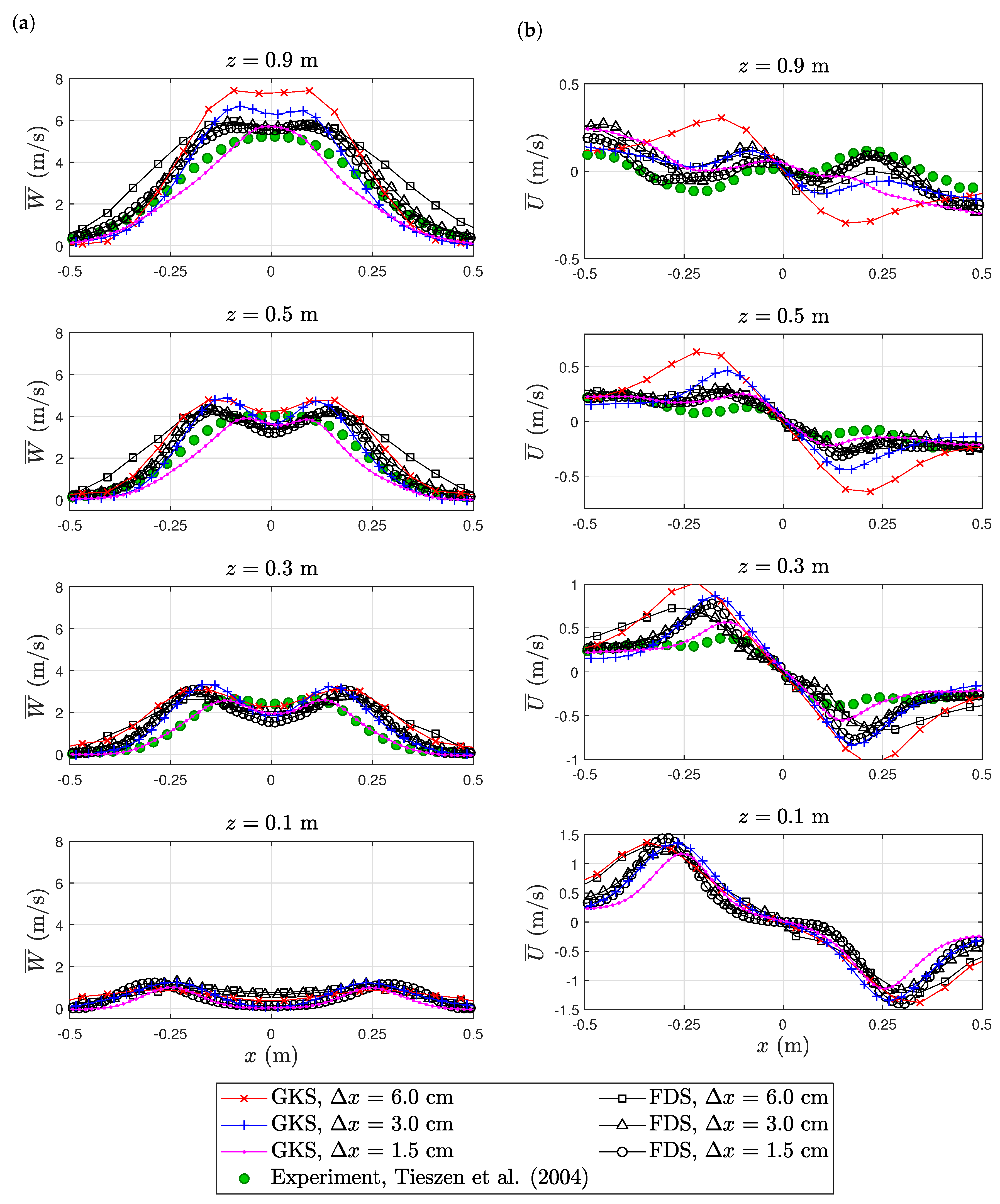
For the sake of validation, time averaged profiles through the flame were collected at different heights as given in [78]. Two velocity components were considered here. The vertical velocity component along the vector of gravitational acceleration is called axial velocity W, because the flame should in theory show a rotational symmetry. The second component is the radial velocity. For profiles along the x-axis, the radial velocity corresponds to the horizontal velocity U (except of the sign). The circumferential velocity component was not considered here, because the flames were not rotating, and consequently, this velocity component was not measured during the experiment. Any present circumferential velocities in the simulations would be due to insufficient averaging.
During the initial comparison of the measured and simulated data, it became obvious that the experimental data were not centered properly. In order to correct for this, we shifted all experimental results for this test case by in the negative x-direction. This value was obtained by computing the normalized first moment of the vertical velocity distribution, i.e.,
for all available data points in the experimental dataset. This procedure centered the experimental data and made comparison with the centered simulations consistent.
The axial velocities of both simulations show a reasonable agreement to the experimental data for both FDS and GKS; see Figure 7a. FDS tended to over-estimate the plume width, while GKS tended to underpredict the width, especially at higher resolution. Both simulations featured a velocity drop in the center of the flame that was not present in the experimental data. In terms of maximal velocity magnitude, FDS tended to over-estimate and GKS to under-estimate. The radial velocity profiles of both simulations showed the measured flow from the inside to the outside; see Figure 7b. The experimental data featured a strong peak in radial velocity at about cm. The strength of this peak was only captured by the coarse FDS simulation. Both the fine grid FDS and GKS simulation did not show such a strong peak.
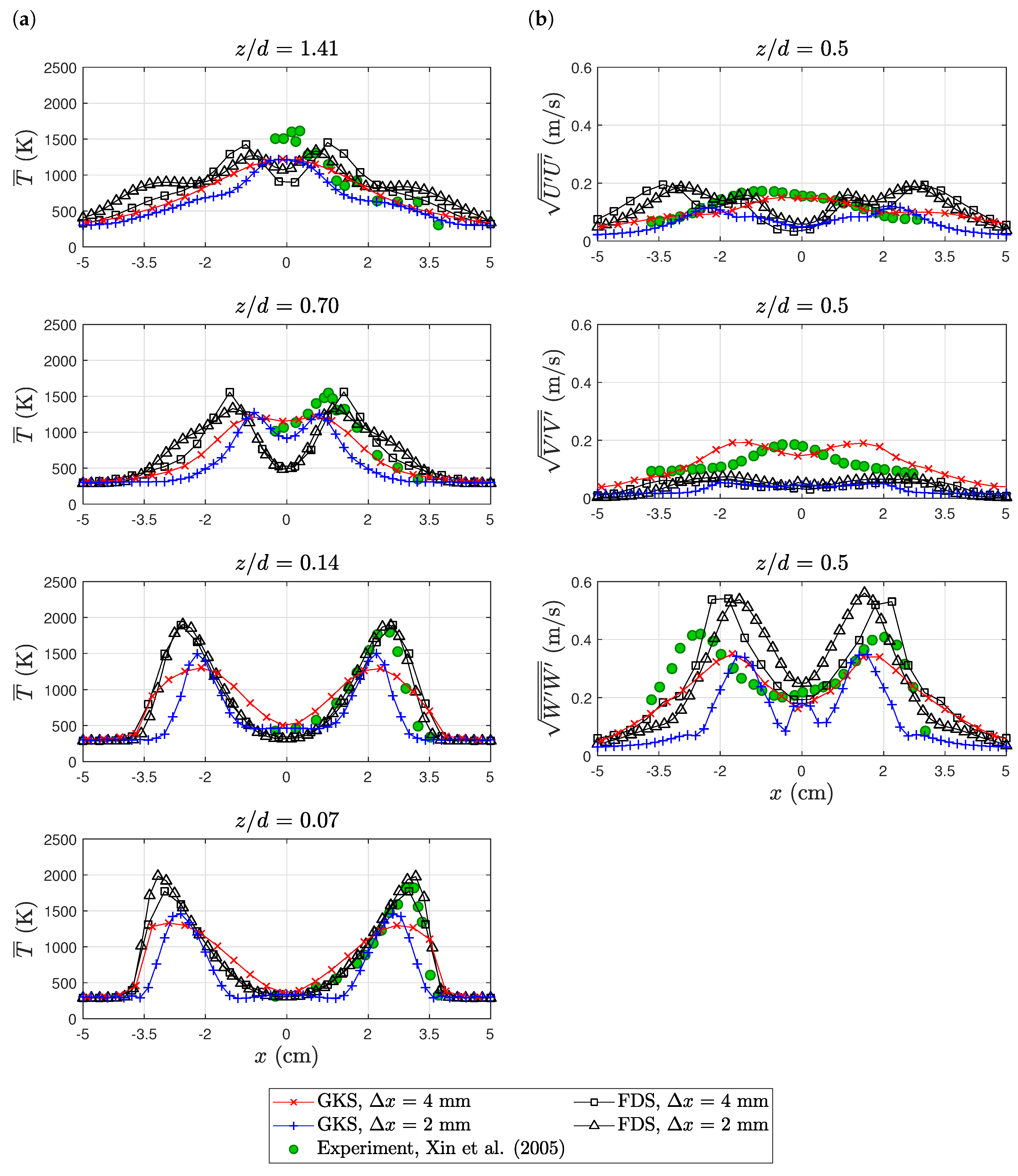
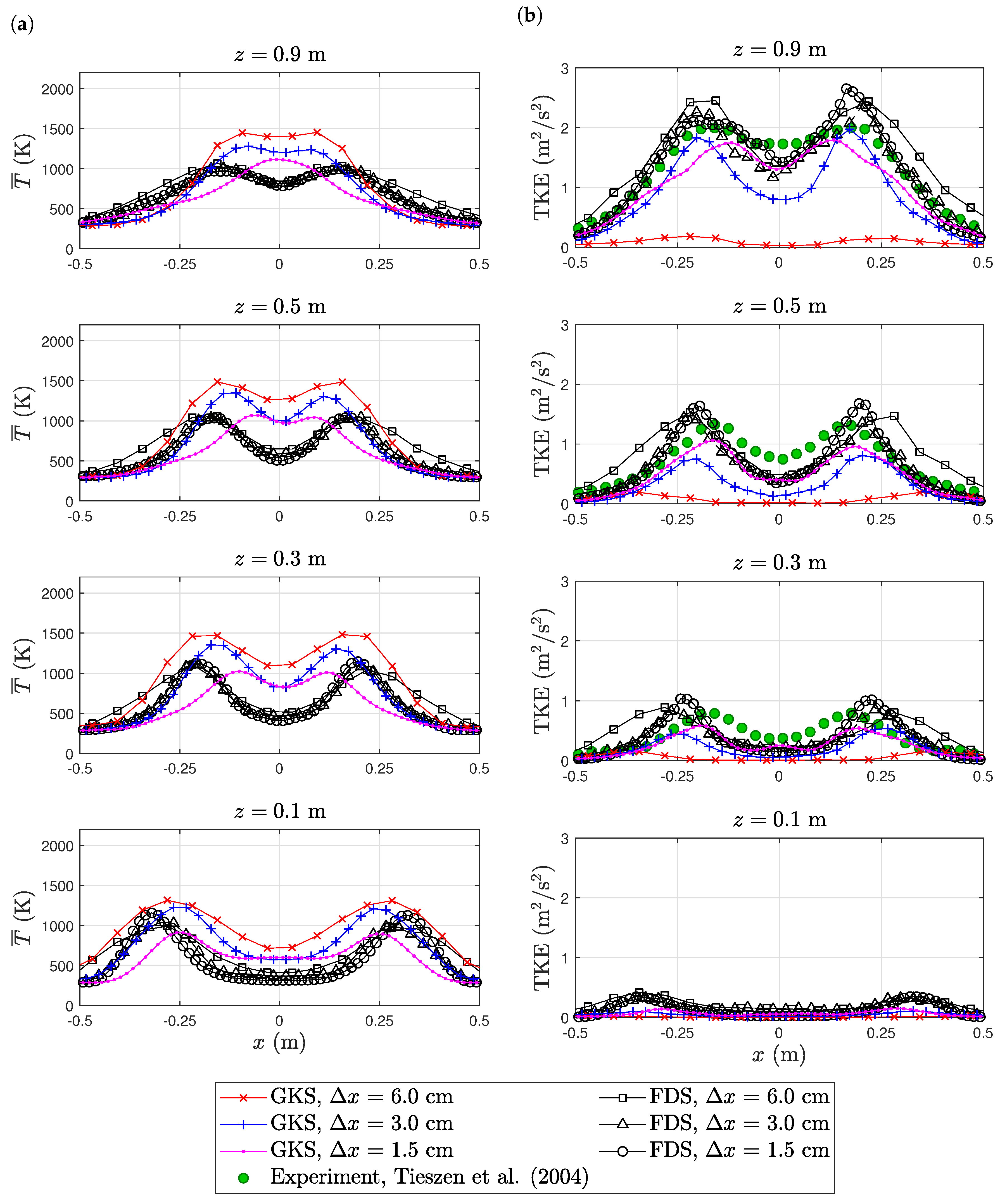
The experimental temperature profiles are only reported for the positive x-axis. The absolute temperature magnitude was under-predicted by GKS, while FDS obtained a good agreement; see Figure 8a. In accordance with the axial velocity profiles, the fine GKS simulation under-predicted the flame width. FDS on the other hand captured nearly the correct flame width with a slight tendency to over-predict. The magnitude of the root-mean-squared vertical (axial) velocity fluctuations was captured with acceptable accuracy; see Figure 8b. The shape of the profiles deviated substantially from the experiment for all simulations. GKS showed less turbulence than FDS.
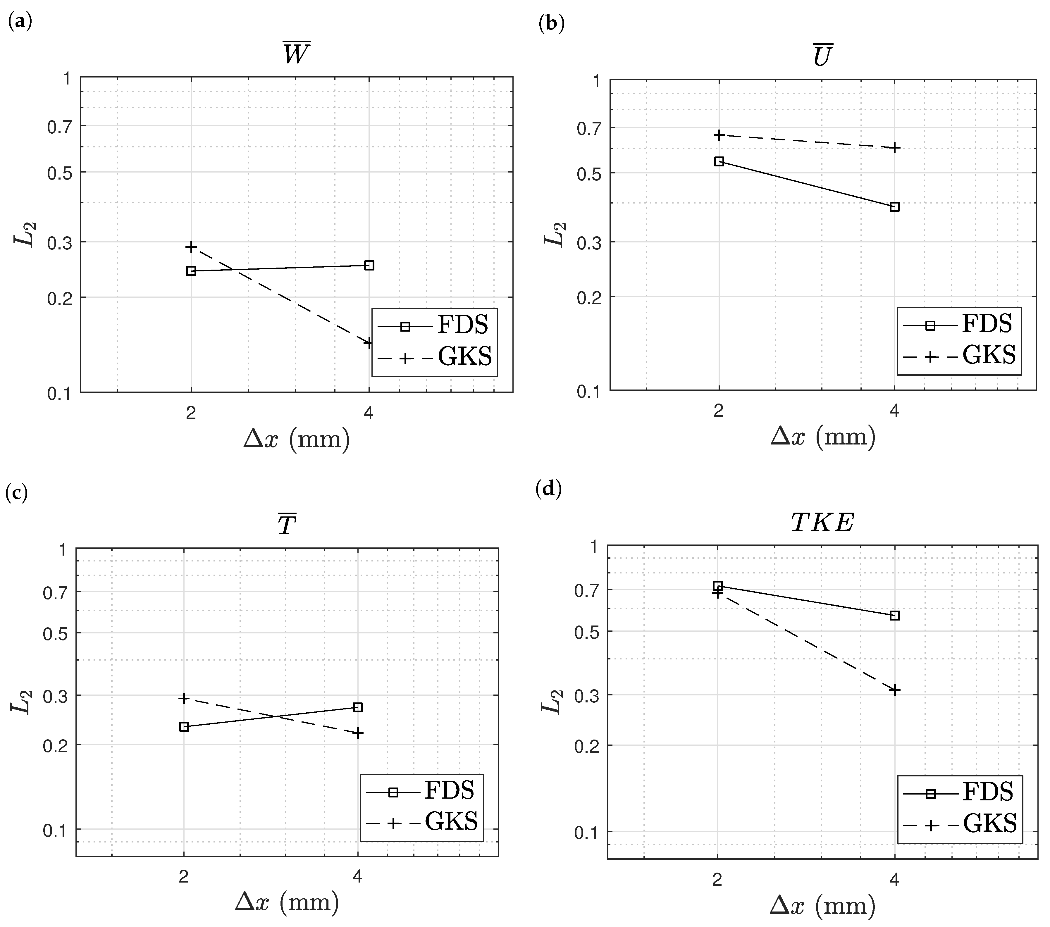
In addition to the profiles, we measured the quality of the simulations in terms of deviation from the experimental data. For the generic quantity , the deviation to was computed as:
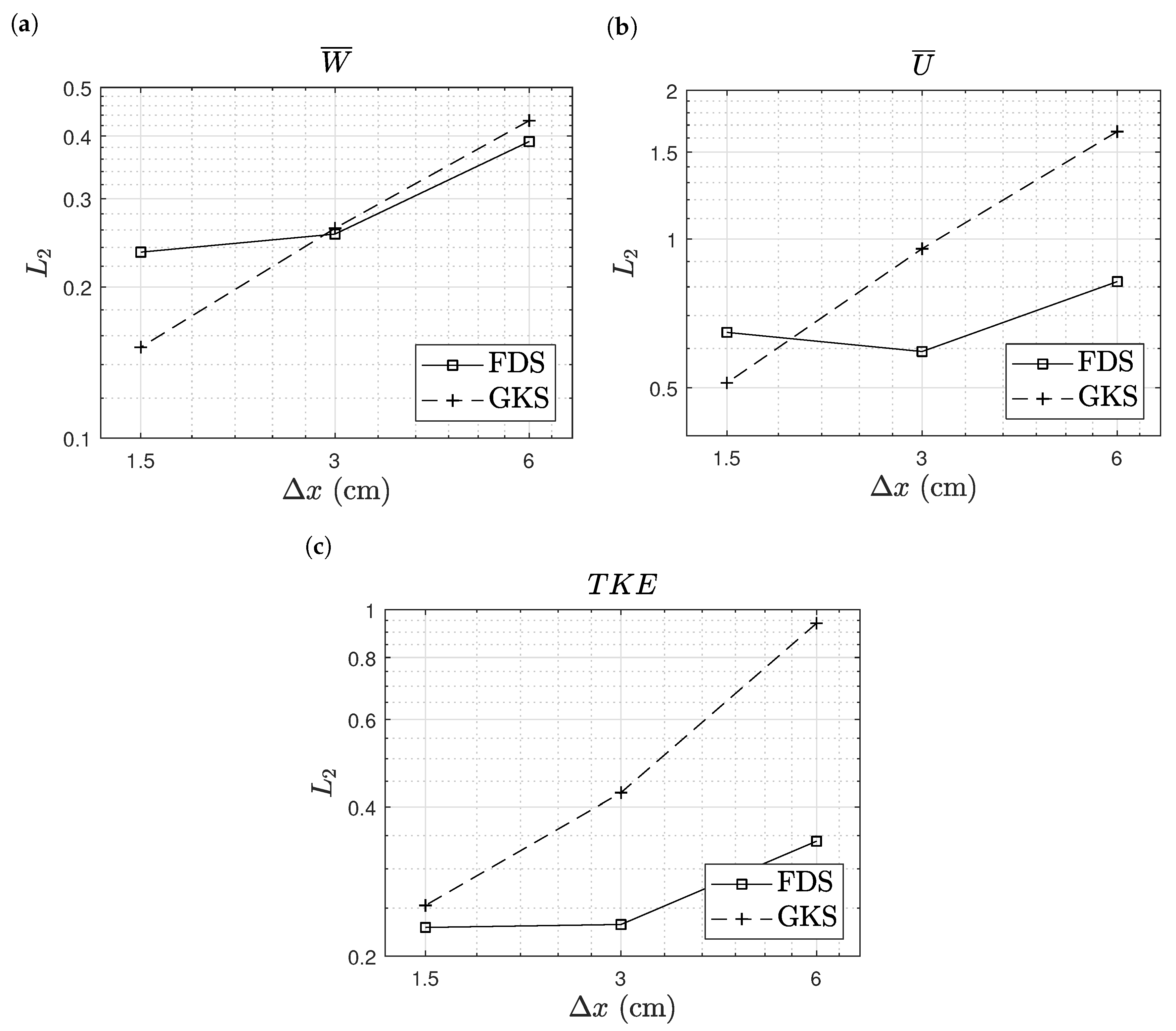
where the simulations results are interpolated linearly towards the location of the experimental data. The sums therein were computed over all grid points on all heights. The deviations for velocities, temperature, and turbulent kinetic energy are shown in Figure 9. A prevalent accuracy between the two methods cannot be found. Furthermore, no substantial improvement in accuracy with refinement was observed for the two simulation methods. In this metric, the GKS results even deviated more from the experimental data with refinement. Nevertheless, the overall accuracy of both methods is comparable. Hence, these results show the general applicability of GKS for the simulation of fire, while some deficiencies in predicting the maximal flame temperature with respect to FDS were observed.
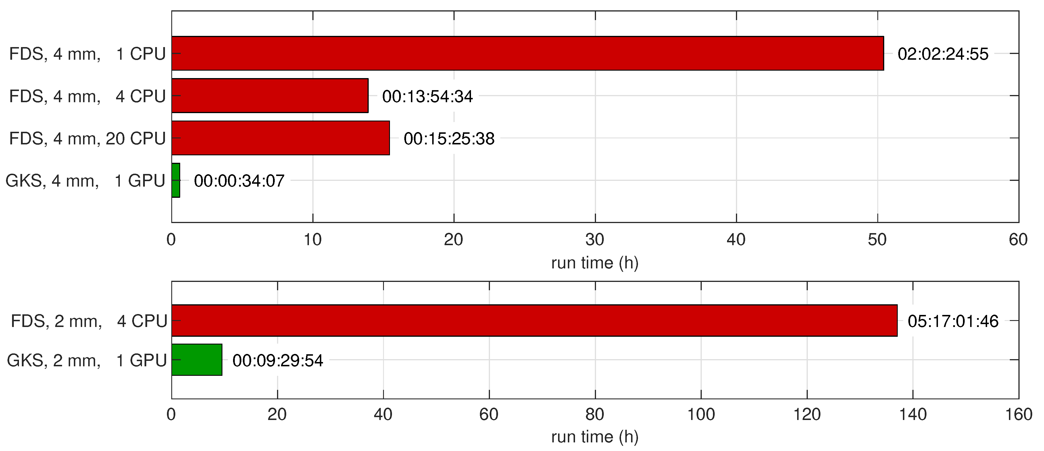
Finally, we compared the absolute times to the solution for both FDS and GKS; see Figure 10. FDS was run on a single CPU core, four cores, and twenty cores. All cores were in the same computer node, which was equipped with two ten-core INTEL Xeon E5-2640v4 CPUs. While using four cores brought a substantial speedup, using more cores brought no further improvement in this experiment. GKS was run on a single NVIDIA Tesla P100 GPGPU. While FDS required between several hours and multiple days to compute twenty seconds of real-time in the simulation, GKS terminated in about half an hour on the coarse grid and nine and a half hours for the fine grid. This resulted in a speedup of about 24 for the coarse and 16 for the fine simulation, demonstrating the capabilities of massively parallel implementations on GPGPUs. While one could argue that the FLOPS rate of the used CPU was substantially lower than of the GPGPU and one should rescale the corresponding wall-clock times accordingly, we note that the inherent FDS solvers cannot utilize the GPGPU architecture, and thus, the GKS has the advantage to benefit from this many-core architecture. In addition, the scalability of the GKS on massively parallel CPU-hardware bears no special challenges, but was not addressed in this work.
6.3. Sandia Flame
The second test case was experimentally investigated at Sandia National Laboratory, Albuquerque, New Mexico, USA, and published by Tieszen et al. [81,82]. This second test had a similar setup to the Purdue flame, but took place at a much larger scale. The burner now had a diameter of one meter. We considered only Test 24 of the Sandia flame experimental series. It was characterized by a total heat release rate of with a methane density of and a mass flow rate of . The properties of air were the same as for the Purdue flame. The flow domain covered . Three uniform discretizations with cm, cm and cm were considered. For this test case, the temperature and heat release rate limiters were activated choosing and . Both limiters were used to stabilize the simulation. The value for was chosen by successively increasing the value, until the simulation remained stable. The value for was taken from FDS Version 5 [69], which also includes this limiter. The justification for this limit is physically based on a scaling analysis for pool fires, which suggested that the spatial average of the heat release rate of fires is about [83].
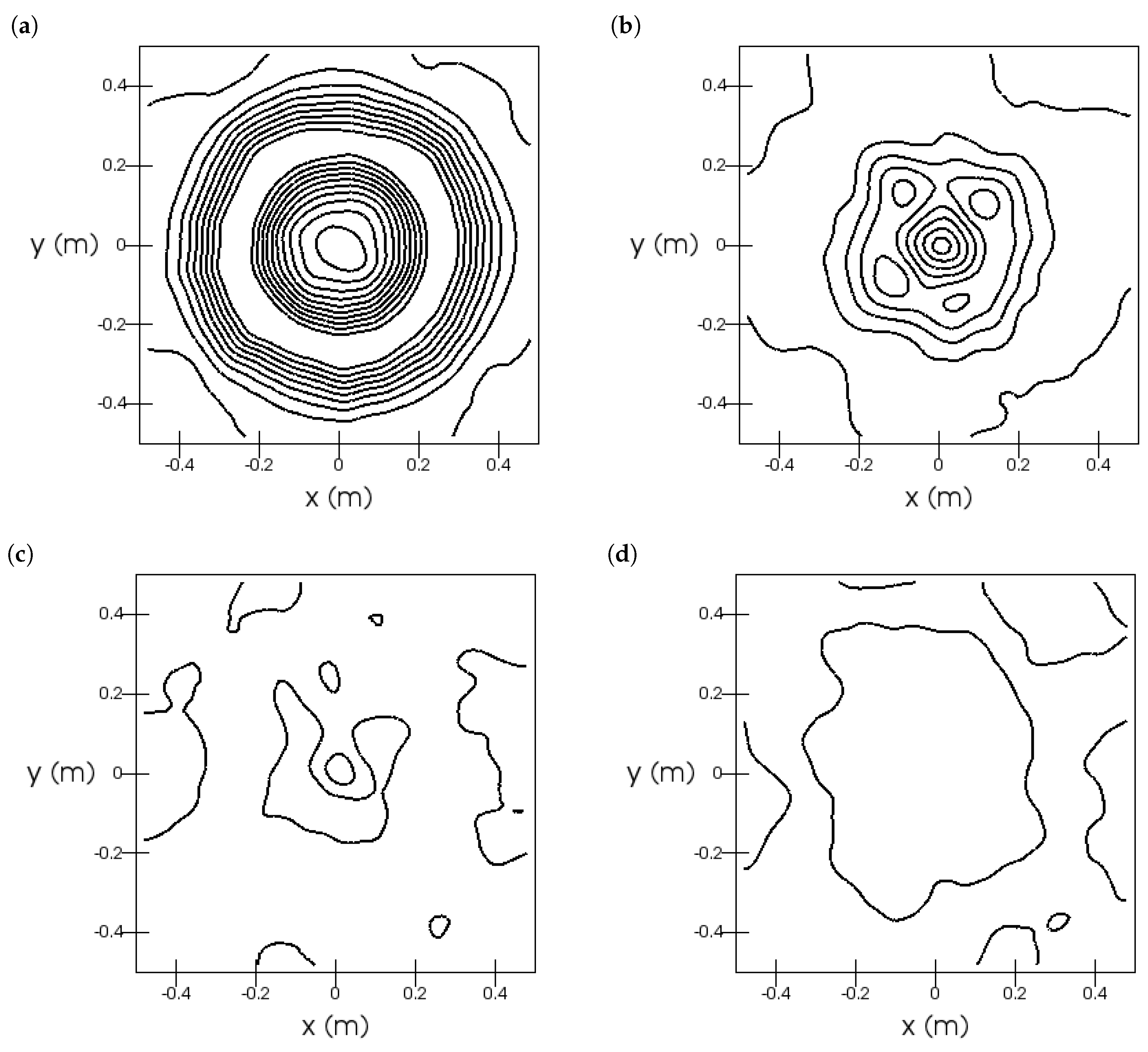
The instantaneous temperature fields of both FDS and GKS simulations at the mid-planes for the highest resolution are shown in Figure 11. GKS appeared to be more dissipative than FDS, which is also confirmed below. The maximal temperatures were similar. FDS showed only a small dependence on the spatial resolution; see the time averaged vertical (axial) velocity profiles Figure 12a. FDS also captured the maximal velocity of the experiment well, but predicted a slightly broader plume. GKS, on the other hand, showed a larger deviation between the three spatial resolutions. At m, the experimental profile was matched almost exactly for the highest resolution. In the higher profiles, GKS tended towards a slightly thinner profile compared to the experimental data. In the radial velocity profiles, we found an even stronger dependence on the spatial resolution, but the profiles converged towards the experimental data; see Figure 12b. Temperature profiles were not reported in the experiment, such that only FDS and GKS are compared in Figure 13a. The FDS profiles of all three resolutions nearly coincided, while the GKS results showed a strong dependence on spatial resolution. The turbulent kinetic energy was probably the most interesting profile when considering the finding in Figure 11. At a height of cm above the burner, GKS predicted near to no turbulence. Here, we saw a clear difference from the FDS results, which was consistent with the instantaneous temperature fields. The coarsest resolution remained at a very low level of turbulence at all heights. The higher resolutions showed more turbulence and seemed to converge towards the experimental data. FDS delivered the right level of turbulence for the three spatial resolutions, but the width of the plume was over-estimated.
Similar to the Purdue flame test case, we also present the deviations between simulations and experimental data; see Figure 14. For this test case, we saw a clear improvement with a reduced cell size for both methods. For GKS, the deviation on the coarse grid was larger than for FDS. Nevertheless, with refinement, GKS reached similar to or better agreement than the experimental data.
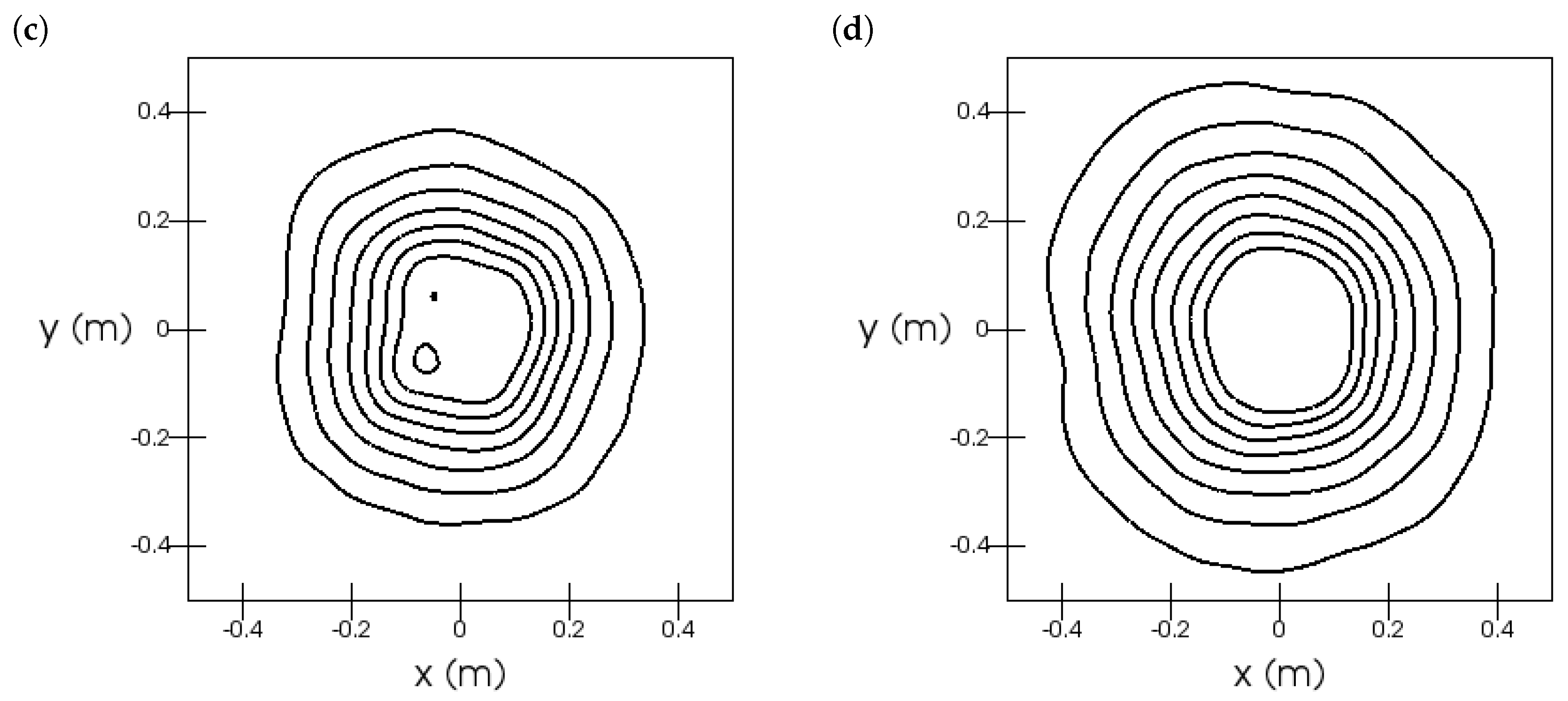
Furthermore, we investigated the radial symmetry of the axial (see Figure 15) and radial (see Figure 16) velocity fields. The velocity fields were not perfectly rotational symmetric.
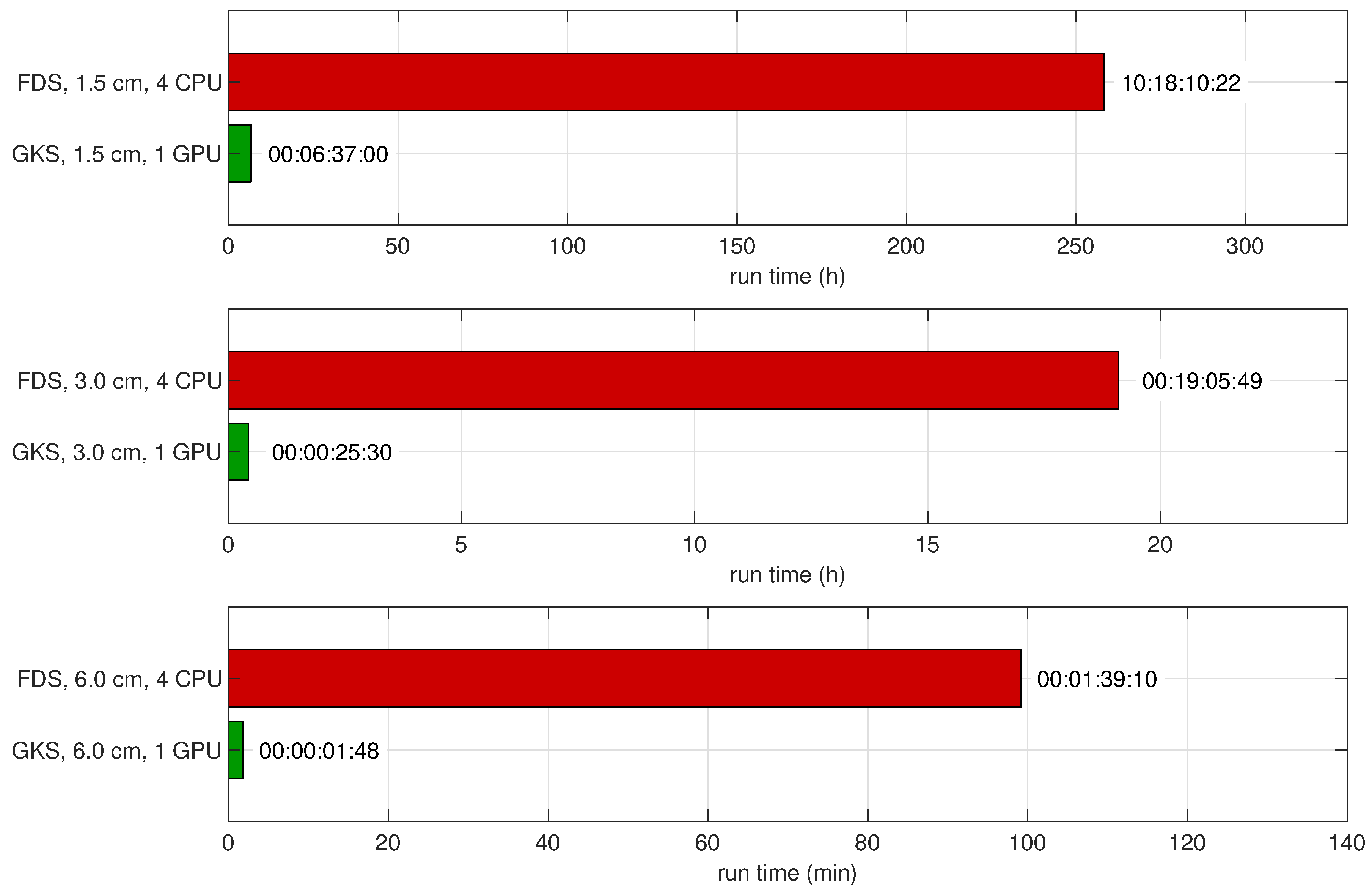
Run times are shown in Figure 17. GKS was between 55 and 40 times faster than FDS. Overall, this test case shows the same tendency as the small-scale Purdue flame: GKS can obtain plausible results for these fire simulations. GKS shows a stronger dependence on the spatial resolution, but is substantially faster, compared to FDS.
7. Conclusions
In the present paper, we demonstrated the efficient usage of gas kinetic schemes for the simulation of fire plumes. To that end, a high performance implementation of GKS for low-Mach number flows in multi-GPGPU environments was presented. The validity of the solver was shown in two dimensions in prior work [45,46]. Here, we showed the extension to three dimensions with an update rate on a single GPGPU of 300 million cell updates per second. On multi-GPU architectures, we demonstrated a high parallel efficiency of over for up to 32 GPGPUs, enabled by communication hiding. The flow solver was augmented by a simple combustion model based on partial mixing and instantaneous reaction for the one-step methane combustion.
The present GKS was validated for three-dimensional, turbulent natural convection, where it showed good agreement with experimental data for first- and second-order statistics. The present fire model was tested on the simulation of two fire plume simulations, one on a small scale and one on a large scale. We presented validation against experimental data and comparison to the standard software FDS. Both tests showed consistent results: The overall magnitudes of temperature and velocity were captured well by the present GKS. For FDS, the results at different spatial resolutions nearly coincided. A limitation of the present approach was that GKS showed substantial deviations between the results for different spatial resolutions. However, the results converged to the experimental data. We assum that the strong dependence on spatial resolution is due to the simple turbulence and combustion models in the present GKS, while FDS features more elaborate models. Future investigations are required to investigate this. Even though the accuracy of the results is slightly lower, we demonstrated substantial speed-ups of more than an order of magnitude in time to solution with respect to FDS.
We conclude that, despite the presented shortcomings, GKS is a viable candidate for the simulation of fire. The focus of future research in this direction has to include advanced turbulence and combustion modeling.
Author Contributions
Conceptualization, S.L. and M.K.; investigation, S.L.; methodology, S.L.; software, S.L.; validation, S.L., M.G. and M.K.; visualization, S.L.; writing, original draft, S.L.; writing, review and editing, M.G. and M.K. All authors have read and agreed to the published version of the manuscript.
Funding
This research was funded by the Deutsche Forschungsgemeinschaft under the framework of the research training group GRK 2075.
Acknowledgments
We thank Martin Salinas-Vázquez for providing the reference data for the turbulent natural convection test case.
Conflicts of Interest
The authors declare no conflict of interest.
Abbreviations
The following abbreviations are used in this manuscript:
| BGK | Bhatnagar–Gross–Krook |
| FDS | Fire Dynamics Simulator |
| GKS | Gas Kinetic Scheme |
| GPGPU | General Purpose Graphics Processing Unit |
| HPC | High Performance Computing |
| LBM | Lattice Boltzmann Method |
| LES | Large Eddy Simulation |
| MPI | Message Passing Interface |
Appendix A. Relations between Mass and Mole Fractions
Mass and mole fractions are defined respectively as:
where and are the mass and amount of the species, respectively. The species components sum up, such that:
Hence, mass and mole fractions sum up to one, i.e.,
The relations between mass and mole fractions are:
with the molar mass of the mixture being:
References
- Quintiere, J.G. Principles of Fire Behavior, 2nd ed.; CRC Press: Boca Raton, FL, USA, 2016. [Google Scholar] [CrossRef]
- Berna, F.; Goldberg, P.; Horwitz, L.K.; Brink, J.; Holt, S.; Bamford, M.; Chazan, M. Microstratigraphic evidence of in situ fire in the Acheulean strata of Wonderwerk Cave, Northern Cape province, South Africa. Proc. Natl. Acad. Sci. USA 2012, 109, E1215–E1220. [Google Scholar] [CrossRef] [PubMed] [Green Version]
- Moore-Bick, M. Grenfell Tower Inquiry: Phase 1 Report. 2019, Volume 4. Available online: https://www.grenfelltowerinquiry.org.uk/phase-1-report (accessed on 17 May 2020).
- Gawad, A.F.A.; Ghulman, H.A. Prediction of Smoke Propagation in a Big Multi-Story Building Using Fire Dynamics Simulator (FDS). Am. J. Energy Eng. 2015, 3, 23. [Google Scholar] [CrossRef] [Green Version]
- Long, X.; Zhang, X.; Lou, B. Numerical simulation of dormitory building fire and personnel escape based on Pyrosim and Pathfinder. J. Chin. Inst. Eng. 2017, 40, 257–266. [Google Scholar] [CrossRef]
- Khan, E.; Ahmed, M.A.; Khan, E.; Majumder, S. Fire Emergency Evacuation Simulation of a shopping mall using Fire Dynamic Simulator (FDS). J. Chem. Eng. 2017, 30, 32–36. [Google Scholar] [CrossRef] [Green Version]
- Guillaume, E.; Dréan, V.; Girardin, B.; Benameur, F.; Koohkan, M.; Fateh, T. Reconstruction of Grenfell Tower fire. Part 3—Numerical simulation of the Grenfell Tower disaster: Contribution to the understanding of the fire propagation and behaviour during the vertical fire spread. Fire Mater. 2019, 46, 605. [Google Scholar] [CrossRef] [Green Version]
- Grosshandler, W.L.; Bryner, N.P.; Madrzykowski, D.M.; Kuntz, K. Report of the Technical Investigation of The Station Nightclub Fire; Technical Report; National Institute of Standards and Technology: Gaithersburg, MD, USA, 2005. [Google Scholar]
- McGrattan, K.B.; Bouldin, C.E.; Forney, G.P. Computer Simulation of the Fires in the World Trade Center Towers, Federal Building and Fire Safety Investigation of the World Trade Center Disaster (NCSTAR 1-5F); Technical Report; National Institute of Standards and Technology: Gaithersburg, MD, USA, 2005. [Google Scholar]
- Barowy, A.M.; Madrzykowski, D.M. Simulation of the Dynamics of a Wind-Driven Fire in a Ranch-Style House—Texas; Technical Report; National Institute of Standards and Technology: Gaithersburg, MD, USA, 2012. [Google Scholar]
- Chi, J.H. Using FDS program and an evacuation test to develop hotel fire safety strategy. J. Chin. Inst. Eng. 2014, 37, 288–299. [Google Scholar] [CrossRef]
- McGrattan, K.B.; Hostikka, S.; Floyd, J.; McDermott, R.; Vanella, M. Fire Dynamics Simulator User’s Guide, 6th ed.; NIST Special Publication, National Institute of Standards and Technology: Gaithersburg, MD, USA, 2006. [Google Scholar]
- McGrattan, K.B.; Hostikka, S.; Floyd, J.; McDermott, R.; Vanella, M. Fire Dynamics Simulator Technical Reference Guide: Volume 1: Mathematical Model, 6th ed.; NIST Special Publication, National Institute of Standards and Technology: Gaithersburg, MD, USA, 2006. [Google Scholar]
- McGrattan, K.B.; Hostikka, S.; Floyd, J.; McDermott, R.; Vanella, M. Fire Dynamics Simulator Technical Reference Guide: Volume 2: Verification, 6th ed.; NIST Special Publication, National Institute of Standards and Technology: Gaithersburg, MD, USA, 2006. [Google Scholar]
- McGrattan, K.B.; Hostikka, S.; Floyd, J.; McDermott, R.; Vanella, M. Fire Dynamics Simulator Technical Reference Guide: Volume 3: Validation, 6th ed.; NIST Special Publication, National Institute of Standards and Technology: Gaithersburg, MD, USA, 2006. [Google Scholar]
- Weller, H.G.; Tabor, G.; Jasak, H.; Fureby, C. A tensorial approach to computational continuum mechanics using object-oriented techniques. Comput. Phys. 1998, 12, 620. [Google Scholar] [CrossRef]
- Husted, B.; Li, Y.Z.; Huang, C.; Anderson, J.; Svensson, R.; Ingason, H.; Runefors, M.; Wahlqvist, J. Verification, Validation and Evaluation of FireFOAM as a Tool for Performance Based Design. 2017. Available online: https://www.brandskyddsforeningen.se/globalassets/brandforsk/rapporter-2017/brandforsk_rapport_309_131_firefoam_new.pdf (accessed on 24 October 2019).
- Wickström, U. Temperature Calculation in Fire Safety Engineering; Springer International Publishing: Cham, Switzerland, 2016. [Google Scholar] [CrossRef]
- Peacock, R.D.; Reneke, P.A.; Forney, G.P. CFAST—Consolidated Model of Fire Growth and Smoke Transport (Version 7) Volume 2: User’s Guide; NIST Technical Note 1889v2; National Institute of Standards and Technology: Gaithersburg, MD, USA, 2015. [Google Scholar] [CrossRef]
- Benzi, R.; Succi, S.; Vergassola, M. The lattice Boltzmann equation: Theory and applications. Phys. Rep. 1992, 222, 145–197. [Google Scholar] [CrossRef]
- Chen, S.; Doolen, G.D. Lattice boltzmann method for fluid flows. Annu. Rev. Fluid Mech. 1998, 30, 329–364. [Google Scholar] [CrossRef] [Green Version]
- D’Humières, D.; Ginzburg, I.; Krafczyk, M.; Lallemand, P.; Luo, L.S. Multiple–relaxation–time lattice Boltzmann models in three dimensions. Philos. Trans. R. Soc. Lond. Ser. A Math. Phys. Eng. Sci. 2002, 360, 437–451. [Google Scholar] [CrossRef]
- Geier, M.; Schönherr, M.; Pasquali, A.; Krafczyk, M. The cumulant lattice Boltzmann equation in three dimensions: Theory and validation. Comput. Math. Appl. 2015, 70, 507–547. [Google Scholar] [CrossRef] [Green Version]
- Godenschwager, C.; Schornbaum, F.; Bauer, M.; Köstler, H.; Rüde, U. A framework for hybrid parallel flow simulations with a trillion cells in complex geometries. In Proceedings of the International Conference on High Performance Computing, Networking, Storage and Analysis, Denver, CO, USA, 17–21 November 2013; pp. 1–12. [Google Scholar] [CrossRef]
- Kutscher, K.; Geier, M.; Krafczyk, M. Multiscale simulation of turbulent flow interacting with porous media based on a massively parallel implementation of the cumulant lattice Boltzmann method. Comput. Fluids 2018, 193, 103733. [Google Scholar] [CrossRef]
- Onodera, N.; Idomura, Y. Acceleration of Wind Simulation Using Locally Mesh-Refined Lattice Boltzmann Method on GPU-Rich Supercomputers. In Supercomputing Frontiers; Yokota, R., Wu, W., Eds.; Springer International Publishing: Cham, Switzerland, 2018; pp. 128–145. [Google Scholar]
- Xu, K. A Gas-Kinetic BGK Scheme for the Navier–Stokes Equations and Its Connection with Artificial Dissipation and Godunov Method. J. Comput. Phys. 2001, 171, 289–335. [Google Scholar] [CrossRef]
- Xu, K.; Mao, M.; Tang, L. A multidimensional gas-kinetic BGK scheme for hypersonic viscous flow. J. Comput. Phys. 2005, 203, 405–421. [Google Scholar] [CrossRef]
- May, G.; Srinivasan, B.; Jameson, A. An improved gas-kinetic BGK finite-volume method for three-dimensional transonic flow. J. Comput. Phys. 2007, 220, 856–878. [Google Scholar] [CrossRef]
- Ni, G.; Jiang, S.; Xu, K. Efficient kinetic schemes for steady and unsteady flow simulations on unstructured meshes. J. Comput. Phys. 2008, 227, 3015–3031. [Google Scholar] [CrossRef]
- Xiong, S.; Zhong, C.; Zhuo, C.; Li, K.; Chen, X.; Cao, J. Numerical simulation of compressible turbulent flow via improved gas-kinetic BGK scheme. Int. J. Numer. Methods Fluids 2011, 67, 1833–1847. [Google Scholar] [CrossRef]
- Li, W.; Kaneda, M.; Suga, K. An implicit gas kinetic BGK scheme for high temperature equilibrium gas flows on unstructured meshes. Comput. Fluids 2014, 93, 100–106. [Google Scholar] [CrossRef]
- Pan, D.; Zhong, C.; Li, J.; Zhuo, C. A gas-kinetic scheme for the simulation of turbulent flows on unstructured meshes. Int. J. Numer. Methods Fluids 2016, 82, 748–769. [Google Scholar] [CrossRef]
- Pan, L.; Xu, K.; Li, Q.; Li, J. An efficient and accurate two-stage fourth-order gas-kinetic scheme for the Euler and Navier–Stokes equations. J. Comput. Phys. 2016, 326, 197–221. [Google Scholar] [CrossRef] [Green Version]
- Pan, L.; Xu, K. Two-stage fourth-order gas-kinetic scheme for three-dimensional Euler and Navier–Stokes solutions. Int. J. Comput. Fluid Dyn. 2018, 32, 395–411. [Google Scholar] [CrossRef] [Green Version]
- Ji, X.; Zhao, F.; Shyy, W.; Xu, K. A family of high-order gas-kinetic schemes and its comparison with Riemann solver based high-order methods. J. Comput. Phys. 2018, 356, 150–173. [Google Scholar] [CrossRef] [Green Version]
- Cao, G.; Su, H.; Xu, J.; Xu, K. Implicit high-order gas kinetic scheme for turbulence simulation. Aerosp. Sci. Technol. 2019, 92, 958–971. [Google Scholar] [CrossRef] [Green Version]
- Zhao, F.; Ji, X.; Shyy, W.; Xu, K. Compact higher-order gas-kinetic schemes with spectral-like resolution for compressible flow simulations. Adv. Aerodyn. 2019, 1, 63. [Google Scholar] [CrossRef] [Green Version]
- Su, M.; Xu, K.; Ghidaoui, M. Low-Speed Flow Simulation by the Gas-Kinetic Scheme. J. Comput. Phys. 1999, 150, 17–39. [Google Scholar] [CrossRef] [Green Version]
- Liao, W.; Peng, Y.; Luo, L.S. Gas-kinetic schemes for direct numerical simulations of compressible homogeneous turbulence. Phys. Rev. E Stat. Nonlinear Soft Matter Phys. 2009, 80, 046702. [Google Scholar] [CrossRef] [Green Version]
- Jin, C.; Xu, K.; Chen, S. A Three Dimensional Gas-Kinetic Scheme with Moving Mesh for Low-Speed Viscous Flow Computations. Adv. Appl. Math. Mech. 2010, 2, 746–762. [Google Scholar] [CrossRef] [Green Version]
- Chen, S.; Jin, C.; Li, C.; Cai, Q. Gas-kinetic scheme with discontinuous derivative for low speed flow computation. J. Comput. Phys. 2011, 230, 2045–2059. [Google Scholar] [CrossRef]
- Wang, P.; Guo, Z. A semi-implicit gas-kinetic scheme for smooth flows. Comput. Phys. Commun. 2016, 205, 22–31. [Google Scholar] [CrossRef]
- Zhou, D.; Lu, Z.; Guo, T. A Gas-Kinetic BGK Scheme for Natural Convection in a Rotating Annulus. Appl. Sci. 2018, 8, 733. [Google Scholar] [CrossRef] [Green Version]
- Lenz, S.; Krafczyk, M.; Geier, M.; Chen, S.; Guo, Z. Validation of a two-dimensional gas-kinetic scheme for compressible natural convection on structured and unstructured meshes. Int. J. Therm. Sci. 2019, 136, 299–315. [Google Scholar] [CrossRef]
- Lenz, S.; Geier, M.; Krafczyk, M. An explicit gas kinetic scheme algorithm on non-uniform Cartesian meshes for GPGPU architectures. Comput. Fluids 2019, 186, 58–73. [Google Scholar] [CrossRef]
- Xu, K.; Huang, J.C. A unified gas-kinetic scheme for continuum and rarefied flows. J. Comput. Phys. 2010, 229, 7747–7764. [Google Scholar] [CrossRef]
- Xu, K.; Huang, J.C. An improved unified gas-kinetic scheme and the study of shock structures. IMA J. Appl. Math. 2011, 76, 698–711. [Google Scholar] [CrossRef]
- Huang, J.C.; Xu, K.; Yu, P. A Unified Gas-Kinetic Scheme for Continuum and Rarefied Flows II: Multi-Dimensional Cases. Commun. Comput. Phys. 2012, 12, 662–690. [Google Scholar] [CrossRef]
- Huang, J.C.; Xu, K.; Yu, P. A Unified Gas-Kinetic Scheme for Continuum and Rarefied Flows III: Microflow Simulations. Commun. Comput. Phys. 2013, 14, 1147–1173. [Google Scholar] [CrossRef]
- Zhu, Y.; Zhong, C.; Xu, K. Unified gas-kinetic scheme with multigrid convergence for rarefied flow study. Phys. Fluids 2017, 29, 096102. [Google Scholar] [CrossRef] [Green Version]
- Guo, Z.; Xu, K.; Wang, R. Discrete unified gas kinetic scheme for all Knudsen number flows: Low-speed isothermal case. Phys. Rev. E Stat. Nonlinear Soft Matter Phys. 2013, 88, 033305. [Google Scholar] [CrossRef] [Green Version]
- Guo, Z.; Wang, R.; Xu, K. Discrete unified gas kinetic scheme for all Knudsen number flows. II. Thermal compressible case. Phys. Rev. E Stat. Nonlinear Soft Matter Phys. 2015, 91, 033313. [Google Scholar] [CrossRef] [Green Version]
- Zhu, L.; Guo, Z.; Xu, K. Discrete unified gas kinetic scheme on unstructured meshes. Comput. Fluids 2016, 127, 211–225. [Google Scholar] [CrossRef] [Green Version]
- Bo, Y.; Wang, P.; Guo, Z.; Wang, L.P. DUGKS simulations of three-dimensional Taylor–Green vortex flow and turbulent channel flow. Comput. Fluids 2017, 155, 9–21. [Google Scholar] [CrossRef]
- Tao, S.; Zhang, H.; Guo, Z.; Wang, L.P. A combined immersed boundary and discrete unified gas kinetic scheme for particle–fluid flows. J. Comput. Phys. 2018, 375, 498–518. [Google Scholar] [CrossRef] [Green Version]
- Zhang, C.; Yang, K.; Guo, Z. A discrete unified gas-kinetic scheme for immiscible two-phase flows. Int. J. Heat Mass Transf. 2018, 126, 1326–1336. [Google Scholar] [CrossRef] [Green Version]
- Bhatnagar, P.L.; Gross, E.P.; Krook, M. A Model for Collision Processes in Gases. I. Small Amplitude Processes in Charged and Neutral One-Component Systems. Phys. Rev. 1954, 94, 511–525. [Google Scholar] [CrossRef]
- NVIDIA. CUDA C Programming Guide; NVIDIA: Santa Clara, CA, USA, 2018. [Google Scholar]
- Sanders, J.; Kandrot, E. CUDA by Example: An Introduction to General-Purpose GPU Programming, 3rd ed.; Addison-Wesley: Upper Saddle River, NJ, USA, 2011. [Google Scholar]
- Smagorinsky, J. General circulation experiments with the primitive equations. Mon. Weather Rev. 1963, 91, 99–164. [Google Scholar] [CrossRef]
- iRMB. VirtualFluids. Available online: https://www.tu-braunschweig.de/irmb/forschung/virtualfluids (accessed on 17 May 2020).
- Deakin, T.; Price, J.; Martineau, M.; McIntosh-Smith, S. GPU-STREAM v2.0: Benchmarking the Achievable Memory Bandwidth of Many-Core Processors Across Diverse Parallel Programming Models. In High Performance Computing; Taufer, M., Mohr, B., Kunkel, J.M., Eds.; Lecture Notes in Computer Science; Springer International Publishing: Cham, Switzerland, 2016; Volume 9945, pp. 489–507. [Google Scholar]
- Obrecht, C.; Kuznik, F.; Tourancheau, B.; Roux, J.J. Multi-GPU implementation of the lattice Boltzmann method. Comput. Math. Appl. 2013, 65, 252–261. [Google Scholar] [CrossRef]
- Calore, E.; Marchi, D.; Schifano, S.F.; Tripiccione, R. Optimizing communications in multi-GPU Lattice Boltzmann simulations. In Proceedings of the 2015 International Conference on High Performance Computing Simulation (HPCS), Amsterdam, The Netherlands, 20–24 July 2015; pp. 55–62. [Google Scholar] [CrossRef]
- Robertsén, F.; Westerholm, J.; Mattila, K. Lattice Boltzmann Simulations at Petascale on Multi-GPU Systems with Asynchronous Data Transfer and Strictly Enforced Memory Read Alignment. In Proceedings of the 2015 23rd Euromicro International Conference on Parallel, Distributed, and Network-Based Processing, Turku, Finland, 4–6 March 2015; pp. 604–609. [Google Scholar] [CrossRef]
- Lian, Y.S.; Xu, K. A Gas-Kinetic Scheme for Multimaterial Flows and Its Application in Chemical Reactions. J. Comput. Phys. 2000, 163, 349–375. [Google Scholar] [CrossRef] [Green Version]
- Li, Q.; Fu, S.; Xu, K. A compressible Navier–Stokes flow solver with scalar transport. J. Comput. Phys. 2005, 204, 692–714. [Google Scholar] [CrossRef]
- McGrattan, K.; Hostikka, S.; Floyd, J.; Baum, H.; Rehm, R. Fire Dynamics Simulator (Version 5): Technical Reference Guide; NIST Special Publication, National Institute of Standards and Technology NIST: Gaithersburg, MD, USA, 2007. [Google Scholar]
- Tian, Y.S.; Karayiannis, T.G. Low turbulence natural convection in an air filled square cavity: Part I: The thermal and fluid flow fields. Int. J. Heat Mass Transf. 2000, 43, 849–866. [Google Scholar] [CrossRef]
- Tian, Y.S.; Karayiannis, T.G. Low turbulence natural convection in an air filled square cavity: Part II: The turbulence quantities. Int. J. Heat Mass Transf. 2000, 43, 867–884. [Google Scholar] [CrossRef]
- Salinas-Vázquez, M.; Vicente, W.; Martínez, E.; Barrios, E. Large eddy simulation of a confined square cavity with natural convection based on compressible flow equations. Int. J. Heat Fluid Flow 2011, 32, 876–888. [Google Scholar] [CrossRef]
- De Vahl Davis, G. Natural convection of air in a square cavity: A bench mark numerical solution. Int. J. Numer. Methods Fluids 1983, 3, 249–264. [Google Scholar] [CrossRef]
- Vierendeels, J.; Merci, B.; Dick, E. Benchmark solutions for the natural convective heat transfer problem in a square cavity with large horizontal temperature differences. Int. J. Numer. Methods Heat Fluid Flow 2003, 13, 1057–1078. [Google Scholar] [CrossRef]
- Vierendeels, J.; Merci, B.; Dick, E. Numerical study of natural convective heat transfer with large temperature differences. Int. J. Numer. Methods Heat Fluid Flow 2001, 11, 329–341. [Google Scholar] [CrossRef]
- Tian, C.T.; Xu, K.; Chan, K.L.; Deng, L.C. A three-dimensional multidimensional gas-kinetic scheme for the Navier–Stokes equations under gravitational fields. J. Comput. Phys. 2007, 226, 2003–2027. [Google Scholar] [CrossRef] [Green Version]
- Hunt, J.; Wray, A.; Moin, P. Eddies, Streams, and Convergence Zones in Turbulent Flow; Center for Turbulence Research Proceedings of the Summer Program: Stanford, CA, USA, 1988. [Google Scholar]
- Xin, Y.; Gore, J.; McGrattan, K.; Rehm, R.; Baum, H. Fire dynamics simulation of a turbulent buoyant flame using a mixture-fraction-based combustion model. Combust. Flame 2005, 141, 329–335. [Google Scholar] [CrossRef]
- Fire Dynamics Simulator–GitHub. Available online: https://github.com/firemodels/fds (accessed on 28 January 2020).
- Deardorff, J.W. Stratocumulus-capped mixed layers derived from a three-dimensional model. Bound. Lay. Meteorol. 1980, 18, 495–527. [Google Scholar] [CrossRef]
- Tieszen, S.R.; O’Hern, T.J.; Schefer, R.W.; Weckman, E.J.; Blanchat, T.K. Experimental study of the flow field in and around a one meter diameter methane fire. Combust. Flame 2002, 129, 378–391. [Google Scholar] [CrossRef]
- Tieszen, S.R.; O’Hern, T.J.; Weckman, E.J.; Schefer, R.W. Experimental study of the effect of fuel mass flux on a 1-m-diameter methane fire and comparison with a hydrogen fire. Combust. Flame 2004, 139, 126–141. [Google Scholar] [CrossRef]
- Orloff, L.; de Ris, J. Froude modeling of pool fires. Symp. Int. Combust. 1982, 19, 885–895. [Google Scholar] [CrossRef]
Figure 1.
Multi-GPGPU communication pattern in two dimensions: The communication in the three directions is performed sequentially in the order x-y-z. The highlighted cell shows the information transport over diagonals.
Figure 1.
Multi-GPGPU communication pattern in two dimensions: The communication in the three directions is performed sequentially in the order x-y-z. The highlighted cell shows the information transport over diagonals.

Figure 2.
Multi-GPGPU communication hiding: The cell faces independent of the receive ghost cells are processed concurrently with the communication and the evaluation of the remaining cell faces.
Figure 2.
Multi-GPGPU communication hiding: The cell faces independent of the receive ghost cells are processed concurrently with the communication and the evaluation of the remaining cell faces.

Figure 3.
Multi-GPGPU: parallel efficiency for weak scaling (a) and strong scaling (b).

Figure 4.
3D square cavity: (a) Non-uniform grid for the GKS simulations with four levels. (b) Contour of the Q criterion at . Grey contour: simulation by Salinas-Vázquez et al. [72]; green Contour: present GKS simulation; the grey contour shows additional turbulence at the top and bottom walls, which is not seen in the present simulation.

Figure 5.
3D square cavity: velocity profiles at heights , , and from bottom to top: (a) Vertical velocity profiles. For visualization, the profiles are shifted by . (b) Horizontal velocity profiles. For visualization, the profiles are shifted by . Experimental values from Tian and Karayiannis [70] and simulation values from Salinas-Vázquez et al. [72].

Figure 6.
3D square cavity: temperature and velocity fluctuation profiles at heights , and from bottom to top: (a) Temperature profiles. For visualization, the profiles are shifted by one. (b) Vertical velocity fluctuation profiles. For visualization, the profiles are shifted by . Experimental values from Tian and Karayiannis [70] and simulation values from Salinas-Vázquez et al. [72].

Figure 7.
Purdue flame: profiles of axial (vertical) velocity (a) and radial (horizontal) velocity (b). The experimental data are available online at https://github.com/firemodels/exp/tree/master/Purdue_Flames.
Figure 7.
Purdue flame: profiles of axial (vertical) velocity (a) and radial (horizontal) velocity (b). The experimental data are available online at https://github.com/firemodels/exp/tree/master/Purdue_Flames.

Figure 8.
Purdue flame: temperature (a) and velocity fluctuation (b) profiles. The experimental data are available online at https://github.com/firemodels/exp/tree/master/Purdue_Flames.
Figure 8.
Purdue flame: temperature (a) and velocity fluctuation (b) profiles. The experimental data are available online at https://github.com/firemodels/exp/tree/master/Purdue_Flames.

Figure 9.
Purdue flame: deviation of the simulation results from the experimental data. Axial velocity (a), radial velocity (b), temperature (c) and turbulent kinetic energy (d).
Figure 9.
Purdue flame: deviation of the simulation results from the experimental data. Axial velocity (a), radial velocity (b), temperature (c) and turbulent kinetic energy (d).

Figure 10.
Purdue flame: time required for FDS and GKS simulations to simulate flame evolution for . The CPUs used are INTEL Xeon E5-2640v4, and the GPUs used are NVIDIA Tesla P100s.
Figure 10.
Purdue flame: time required for FDS and GKS simulations to simulate flame evolution for . The CPUs used are INTEL Xeon E5-2640v4, and the GPUs used are NVIDIA Tesla P100s.

Figure 11.
Sandia flame, Test 24: Instantaneous temperature field computed by FDS (a) and GKS (b) at from the fine simulations with cm.
Figure 11.
Sandia flame, Test 24: Instantaneous temperature field computed by FDS (a) and GKS (b) at from the fine simulations with cm.

Figure 12.
Sandia flame, Test 24: profiles of axial (vertical) velocity (a) and radial(horizontal) velocity (b). The experimental data are available online at https://github.com/firemodels/exp/tree/master/Sandia_Plumes.
Figure 12.
Sandia flame, Test 24: profiles of axial (vertical) velocity (a) and radial(horizontal) velocity (b). The experimental data are available online at https://github.com/firemodels/exp/tree/master/Sandia_Plumes.

Figure 13.
Sandia flame, Test 24: temperature (a) and turbulent kinetic energy (b) profiles. The experimental data are available online at https://github.com/firemodels/exp/tree/master/Sandia_Plumes.
Figure 13.
Sandia flame, Test 24: temperature (a) and turbulent kinetic energy (b) profiles. The experimental data are available online at https://github.com/firemodels/exp/tree/master/Sandia_Plumes.

Figure 14.
Sandia flame, Test 24: deviation of the simulation results from the experimental data. Axial velocity (a), radial velocity (b) and turbulent kinetic energy (c).
Figure 14.
Sandia flame, Test 24: deviation of the simulation results from the experimental data. Axial velocity (a), radial velocity (b) and turbulent kinetic energy (c).

Figure 15.
Sandia flame, Test 24: iso-contours of axial velocity. The sub-figures are at heights (a), (b), (c), and (d). The contours are in the range with a stride of .
Figure 15.
Sandia flame, Test 24: iso-contours of axial velocity. The sub-figures are at heights (a), (b), (c), and (d). The contours are in the range with a stride of .


Figure 16.
Sandia flame, Test 24: iso-contours of radial velocity. The sub-figures are at heights (a), (b), (c), and (d). The contours are in the range with a stride of .
Figure 16.
Sandia flame, Test 24: iso-contours of radial velocity. The sub-figures are at heights (a), (b), (c), and (d). The contours are in the range with a stride of .

Figure 17.
Sandia flame, Test 24: time required for FDS and GKS simulations to simulate flame evolution for . The CPUs used are INTEL Xeon E5-2640v4, and the GPUs used are NVIDIA Tesla P100s.
Figure 17.
Sandia flame, Test 24: time required for FDS and GKS simulations to simulate flame evolution for . The CPUs used are INTEL Xeon E5-2640v4, and the GPUs used are NVIDIA Tesla P100s.

© 2020 by the authors. Licensee MDPI, Basel, Switzerland. This article is an open access article distributed under the terms and conditions of the Creative Commons Attribution (CC BY) license (http://creativecommons.org/licenses/by/4.0/).
Share and Cite
MDPI and ACS Style
Lenz, S.; Geier, M.; Krafczyk, M. Simulation of Fire with a Gas Kinetic Scheme on Distributed GPGPU Architectures. Computation 2020, 8, 50. https://0-doi-org.brum.beds.ac.uk/10.3390/computation8020050
AMA Style
Lenz S, Geier M, Krafczyk M. Simulation of Fire with a Gas Kinetic Scheme on Distributed GPGPU Architectures. Computation. 2020; 8(2):50. https://0-doi-org.brum.beds.ac.uk/10.3390/computation8020050
Chicago/Turabian StyleLenz, Stephan, Martin Geier, and Manfred Krafczyk. 2020. "Simulation of Fire with a Gas Kinetic Scheme on Distributed GPGPU Architectures" Computation 8, no. 2: 50. https://0-doi-org.brum.beds.ac.uk/10.3390/computation8020050
Note that from the first issue of 2016, this journal uses article numbers instead of page numbers. See further details here.