Article

On the Numerical Analysis of Unsteady MHD Boundary Layer Flow of Williamson Fluid Over a Stretching Sheet and Heat and Mass Transfers

1
Department of Mathematics and Applied Mathematics, School of Natural and Mathematical Sciences, University of Venda, P. Bag X5050, Thohoyandou 0950, South Africa
2
Department of Mathematics, University of Zimbabwe, Mt. Pleasant P.O. Box MP167, Zimbabwe
*
Author to whom correspondence should be addressed.
Submission received: 9 April 2020 / Revised: 5 May 2020 / Accepted: 8 May 2020 / Published: 2 June 2020
(This article belongs to the Special Issue Computational Heat, Mass, and Momentum Transfer—II)

Abstract

:
A thorough and detailed investigation of an unsteady free convection boundary layer flow of an incompressible electrically conducting Williamson fluid over a stretching sheet saturated with a porous medium has been numerically carried out. The partial governing equations are transferred into a system of non-linear dimensionless ordinary differential equations by employing suitable similarity transformations. The resultant equations are then numerically solved using the spectral quasi-linearization method. Numerical solutions are obtained in terms of the velocity, temperature and concentration profiles, as well as the skin friction, heat and mass transfers. These numerical results are presented graphically and in tabular forms. From the results, it is found out that the Weissenberg number, local electric parameter, the unsteadiness parameter, the magnetic, porosity and the buoyancy parameters have significant effects on the flow properties.

1. Introduction

The study of non-Newtonian fluids has attracted many researchers owing to its enormous applications in industrial and engineering sectors, especially in manufacturing and processing industries. Unlike Newtonian fluids, Kahshan et al. [1], non-Newtonian fluids are more complicated because there is no single construction relation that can be used to explain them all, Hussanan et al. [2]. The relationship between the shear stress and rate of strain is non-linear at a given temperature and pressure in a non-Newtonian fluid. To this end, these fluids cannot be modelled using the classical Navier-Stokes equations. Non-Newtonian fluids have the ability to: (i) shear-thin or shear thicken, (ii) exhibit thixotropy, (iii) allow stress relaxation, (iv) creep in a nonlinear manner, (v) develop normal stress differences, and (vi) exhibit a threshold for the shear stress before it starts to flow. Many non-Newtonian fluids possess one or more of these characteristics.
Non-Newtonian fluids are generally classified into three main categories, namely: (i) the differential type, (ii) the rate type and (iii) the integral type. The detailed descriptions of each category can be found in Cioranescu et al. [3]. In non-Newtonian fluids, pseudoplastic fluids are the most frequently encountered fluids. But as expected, Navier-stokes equations alone are insufficient to describe the rheological properties of these fluids. Therefore, to overcome this challenge, many rheological models like Maxwell model, Jeffrey model, Ellis model, Power law model, Carreau model, among others, have been developed. The Williamson fluid model is another powerful model used to explain the rheological properties of pseudoplastic fluids. A pseudoplastic is a shear-thinning fluid and has less resistance at high strain rates like polymer solution, paint, blood, plasma. In rheology, shear thinning is the pseudoplastic fluid whose viscosity decreases under shear strain. The shear thinning fluid behaviour is usually exhibited by inks which are used in inkjet printing as discussed by Miccichè et al. [4] and Dybowska-Sarapuk et al. [5].
A lot of authors have investigated the flow of non-Newtonian fluids due to their vast applications especially when with suspensions of nano-sized particle. Some work on nanoparticles was done by Mozaffari et al. [6], Mozaffari et al. [7], Darjani et al. [8] and Xing et al. [9]. Considering a flow underlying spreading surface through a non-Darcian porous medium, Elgazery [10] anlayzed the effects of internal heat generation/absorption of a non-Newtonian Casson fluid with suspension of gold and alumina nanoparticles. Hsiao [11] presented a study for thermal energy extrusion system conversion problem with electric hydromagnetic heat and mass mixed convection of a viscoelastic non-Newtonian Carreau-Nanofluid with radiation and viscous dissipation effects. Khan et al. [12] studied the influence of the nanoparticles and uniform magnetic field on the slip flows in arterial vessels with blood conveyed through hollow arterial tubes described as a third grade non-Newtonian fluid. An investigation on the multislip effects on the magnetohydrodynamic mixed convection unsteady flow of microploar nanofluids over a stretching/shrinking sheet along with radiation in the presence of a heat source was done by Abdal et al. [13]. Adesanya et al. [14] investigated the steady flow of the non-Newtonian fluid via the inclined channel heated isothermally at the boundaries.
Williamson [15] pioneered the discussion of the flow of pseudoplastic materials and proposed a model equation to describe the flow of pseudoplastic fluids and experimentally verified the results. Nadeem et al. [16] presented a paper modelling a two-dimensional Williamson fluid flow over a stretching sheet. Nadeem and Hussain [17] explored the effects of heat transfers on the Williamson fluid over a porous exponentially stretching sheet surface. The study also considered the two cases of heat transfer, namely, the prescribed exponential order surface temperature case and the prescribed exponential order heat flux case. Khan et al. [18] described the effect of thermal radiation on the thin film nanofluid flow of a Williamson fluid over an unsteady stretching surface with variable fluid properties. Ijaz Khan et al. [19] developed a model for a boundary layer stagnation point flow of an electrically conducting Williamson fluid in the presence of a constant magnetic field.
Monica et al. [20] presented an analysis that dealt with the study of stagnation point flow of a Williamson fluid over nonlinearly stretching sheet with thermal radiation. Malik et al. [21] studied the Williamson fluid past a stretching cylinder with combined effects of variable thermal conductivity and heat generation/absorption. Mabood et al. [22] performed an analysis for MHD Williamson nanofluid flow over a continuously moving heated surface with thermal radiation and heat source. Dawar et al. [23] did an analysis of the flow of a Williamson fluid taken over a linear porous stretching sheet under the influence of thermal radiation.
Kurmar et al. [24] carried out a mathematical analysis of two-phase boundary layer flow and heat transfer of a Williamson fluid with particle suspension over a stretching sheet. Shateyi et al. [25] investigated a Casson fluid flow in the presence of free convection of combined heat and mass transfer towards an unsteady permeable stretching sheet with thermal radiation, viscous dissipation and chemical reaction. Hayat et al. [26] studied the unsteady two-dimensional boundary layer flow of an incompressible Williamson fluid over an unsteady permeable stretching surface with thermal radiation. Khan et al. [27] examined the influence of chemically reactive species and mixed convection on the magnetohydrodynamic Williamson nanofluid induced by a nonisothermal cone and plate in a porus medium.
Recently, Panezai et al. [28] examined the influence of thermal radiation on two-dimensional incompressible MHD mixed convective heat transfer flow of Williamson fluid flowing over a porous wedge. Hsu et al. [29] numerically analysed the heat and mass transfer characteristics of the influence of uniform blowing/suction and MHD (magnetohydrodynamic) on the free convection of non-newtonian fluids over a vertical plate in porous media with internal heat generation and soret/dufour effects. Kebede [30] presented an analytic approximation to the heat and mass transfer characteristics of Williamson nanofluid flow. Reddy et al. [31] studied MHD flow and heat transfer characteristics of Williamson nanofluid over a stretching sheet with variable thickness and variable thermal conductivity.
Lastly, Megahed [32] researched on Williamson boundary layer fluid flow and heat transfer due to a nonlinearly stretching sheet. Many researchers have been attracted to study viscous flows due to a stretching sheet. This has been necessitated by their several applications in polymer processing industries, environmental pollution, biological processes and aerodynamic extrusion of plastic sheets, among other applications. Sakiadis [33] pioneered the discussion of the fluid flow due to a stretching surface. Crane [34] extended the work of Sakiadis to study the problem of fluid flow of Blasius type due to a stretching sheet. The literature on the stretching sheet topic is quite extensive and hence cannot be listed here in detail. The most recent works of great researchers regarding the flow over stretching sheet can be found in Hsiao [35,36], Shateyi [37], Sharma et al. [38], Shamashuddin et al. [39], Nagalakshm and Vijaya [40].
Motivated by the above mentioned studies as well as the vast applications of the different types of non-Newtonian fluids, the current study seeks to investigate unsteady free convection boundary layer flow of an electrically conducting Williamson fluid over a stretching sheet. The sheet is saturated with a porous medium under the combined effects of viscous dissipation, chemical reaction, thermal radiation as well as a uniform magnetic field. It is well known that fluid dynamics problems are analysed through material and virtual experimentation, Vedovoto et al. [41]. Material modeling entails the construction of benches and models of the physical problems, as well as instrumentation for gathering information. However, the virtual experimentation requires mathematical modeling which leads to models with differential equations, integral equations and/or intro-differential equations. It is remarked that valuable information about the problem is provided by virtual experimentation. Numeric algorithms and quantitative information about the problem are generated through computational modelling. The data is then used to perform the visualization of the simulation results ad the statistical analysis of the numerical experiment. To that end, the current study also seeks to use the virtual experimentation approach. We are also employing recently developed numerical technique known as the spectral quasi-linearization method. Therefore, novelty of the current paper lies in the application of the numerical technique to solve this two dimensional, unsteady free convection boundary layer flow of an incompressible electrically conducting Williamson fluid over a stretching sheet saturated with a porous medium. The innovation of this study lies in putting together more factors into the basic Williamson fluid model to give a through analysis of the model.

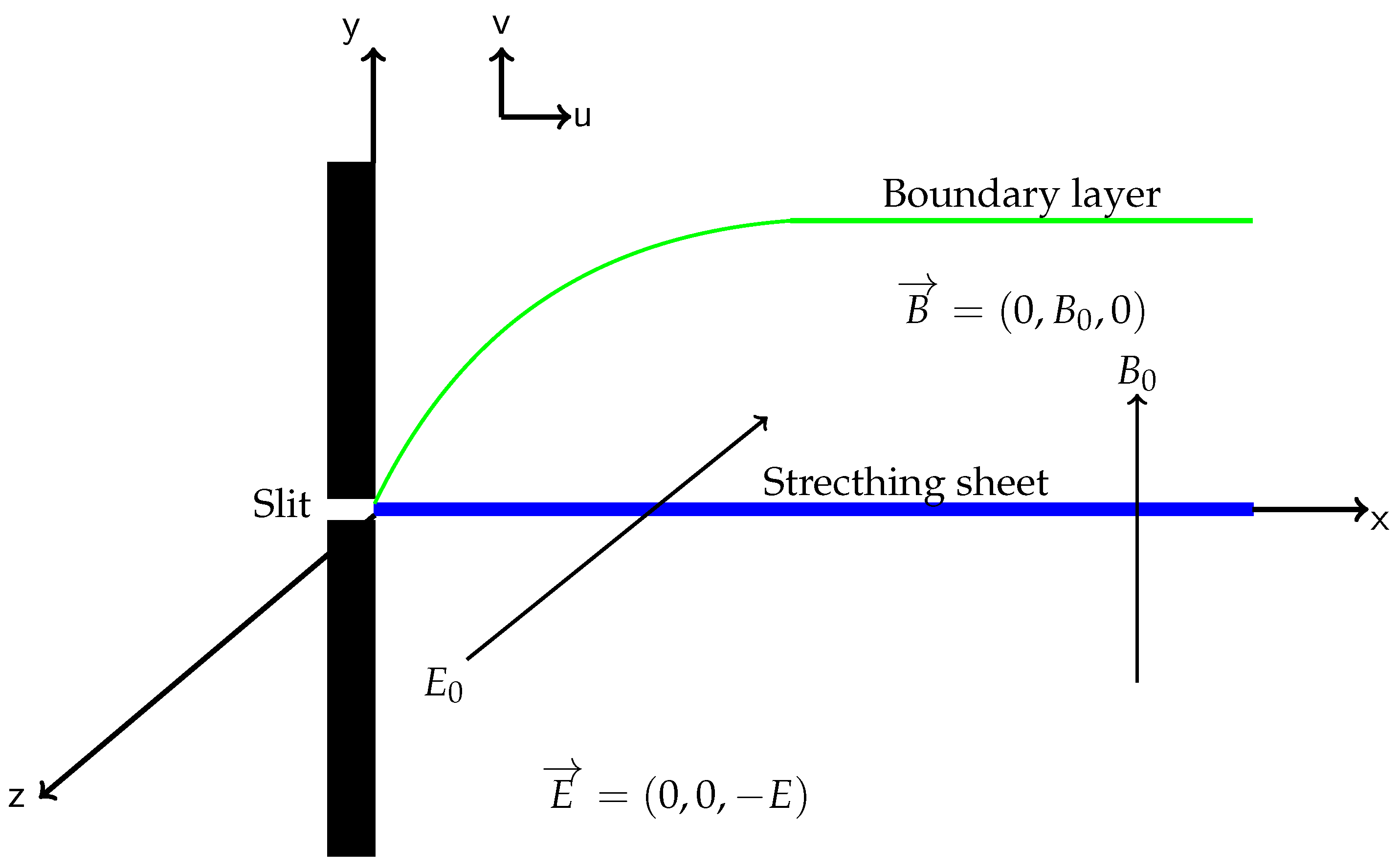
2. Mathematical Formulation

We consider a two dimensional, unsteady free convection boundary layer flow of an incompressible electrically conducting Williamson fluid over a stretching sheet saturated with a porous medium. The x-axis is taken parallel to the stretching sheet and the y-axis is in the vertical direction. We assume that the sheet is moving with a velocity U w = a x 1 c t , where a > 0 is a stretching rate along the x-axis. If a < 0 , then it becomes a shrinking velocity constraint. The the constant c t is such that c t < 1 . A uniform transverse magnetic field B = ( 0 , B 0 , 0 ) and uniform electric field E = ( 0 , 0 , E 0 ) are applied to the flow region as shown in Figure 1. The magnetic Reynolds number is assumed to be much less than unity and hence the induced magnetic field is negligible in comparison to the applied magnetic field. This is made possible by the fact that the fluid is assumed to be slightly conducting. In this study we also neglect the Hall effect/currents. We note that the magnetic field is weaker than the electric field and also that the magnetic field obeys Ohm’s law J ˇ = σ ( E + V ¯ × B ) , where J ˇ is the Joule current, σ is the electrical conductivity and V ¯ is the velocity. We take into account frictional heating in the from of viscous dissipation. Thermal radiation and chemical reaction are also considered in this study. We neglect the induced magnetic field and the hall effect.
The relevant governing flow equations through the conservation laws of mass, linear momentum, energy and mass by using the boundary layer approximations give the following Hayat et al. [26]
u x + v y = 0 , u t + u u x + v u y = ν 2 u y 2 + 2 ν Γ u y 2 u y 2 + g β ( T T ) + g β c ( C C )
+ σ ρ ( E 0 B 0 B 0 2 u ) ,
T t + u T x + v T y = K ρ c p 2 T y 2 + μ ρ c p u y 2 + μ Γ ρ c p u y 3 + σ ρ c p ( β 0 u E 0 ) 2 1 ρ c p q r y ,
C t + u C x + v C y = D 2 C y 2 K r ( C C ) ,
subject to boundary conditions
u ( x , 0 ) = U w , v ( x , 0 ) = V w , T ( x , 0 ) = T w , C ( x , 0 ) = C w , u 0 , T T , C C , as y .
Here u and v are the velocity components in the x and y directions, respectively, ν is the kinematic viscosity, Γ is the relaxation time, g is the acceleration due to gravity, T and C are the fluid temperature and concentration, respectively, T and C are the respective ambient temperature and concentration, β and β c are the respective coefficients of thermal and concentration expansion, σ is the electrical conductivity, ρ is the fluid density, μ is the dynamic viscosity, κ is the permeability parameter, c p is the specific heat at constant pressure, q r is the radiative heat flux, K r is the chemical reaction rate, K is thermal conductivity and lastly, D is the mass diffusivity. V w is expressed by V w = V 0 ( 1 c t ) 1 2 .
As now known, V w express the mass transfer at the surface with V w < 0 for injection and V w > 0 being for suction. The surface temperature T w ( x , t ) and the surface concentration C w ( x , t ) are given respectively as:
T w ( x , t ) = T + a x 2 ν ( 1 c t ) 2 T 0 and C w ( x , t ) = C + a x 2 ν ( 1 c t ) 2 C 0 ,
where c 0 . T 0 ( 0 T 0 T w ) and C 0 ( 0 C 0 C w ) are the reference temperature and concentration respectively.
By employing the Rosseland approximations, we have
q r = 4 σ * 3 k 1 T 4 y ,
where σ * is the Stefan-Boltzmann constant and k 1 is the mean absorption coefficient. Applying Taylor’s series, we have T 4 4 T 3 T 3 T 4 , where T , is the ambient temperature and the energy equation now becomes:
T t + u T x + v T y = 1 ρ c p 16 σ * T 3 3 k 1 + K 2 T y 2 + μ ρ c p u y 2 + μ Γ ρ c p u y 3 + σ ρ c p ( β 0 u E 0 ) 2 .

Similarity Transformation

Following Hayat et al. [26], among others, we introduce the following dimensionless variables.
η = U w x ν y , ψ = ν x U w f ( η ) , θ ( η ) = T T T w T , ϕ ( η ) = C C C w C ,
with the velocity components given by u = ψ y and v = ψ x .
The continuity equation is satisfied and the resulting governing partial differential equations together with the boundary conditions become:
( 1 + 2 W e f ) f + f f ( f ) 2 S f + η 2 f + M 2 ( E 1 f ) + λ 1 θ + λ 2 ϕ = 0 ,
1 P r 1 + 4 R 3 θ + f θ S η 2 θ ( 2 S + f ) θ + E c ( ( f ) 2 + W e ( f ) 3 ) + M 2 E c ( f E 1 ) 2 = 0 ,
1 S c ϕ + f S η 2 ϕ + ( 2 S f γ ) ϕ = 0 .
The corresponding boundary conditions become:
f ( 0 ) = f w , f ( 0 ) = 1 , θ ( 0 ) = 1 , ϕ ( 0 ) = 1 ,
f ( ) 0 , f ( ) 0 θ ( ) 0 , ϕ ( ) 0 ,
where S = c a is the unsteadiness parameter, f w = V 0 a ν is the suction/injection parameter, W e = Γ U w a ν ( 1 c t ) is the Weissenberg number, M 2 = σ B 0 2 ( 1 c t ) ρ a and M is the magnetic field parameter, E 1 = E 0 ( 1 c t ) B 0 a x is the local electric parameter, R = 4 σ * T 3 κ K is the thermal radiation parameter, S c = ν D is the Schmidt number, P r = μ c p K is the Prandtl number, γ = K r ( 1 c t ) a is the chemical reaction parameter, λ 1 = g β T 0 2 a ν is the thermal buoyancy parameter, λ 2 = g β c C 0 2 a ν is the solutal buoyancy parameter, E c = U w 2 c p ( T w T 0 ) is the Eckert number.
The flow characteristics which are of engineering significance are the skin friction coefficient, the local Nusselt number and the Sherwood number. These are respectively, defined as: (Hayat et al. [26])
C f = τ w ρ U w 2 , N u x = x q w K ( T w T ) , S h x = x j w k ( C w C ) .
Upon applying the necessary expressions for τ w , q w , and j w , we get the following:
C f = R e x 1 / 2 [ f ( 0 ) + W e f 2 ( 0 ) ] , N u x = R e x 1 / 2 1 + 4 R 3 θ ( 0 ) , S h x = R e x 1 / 2 ϕ ( 0 ) .

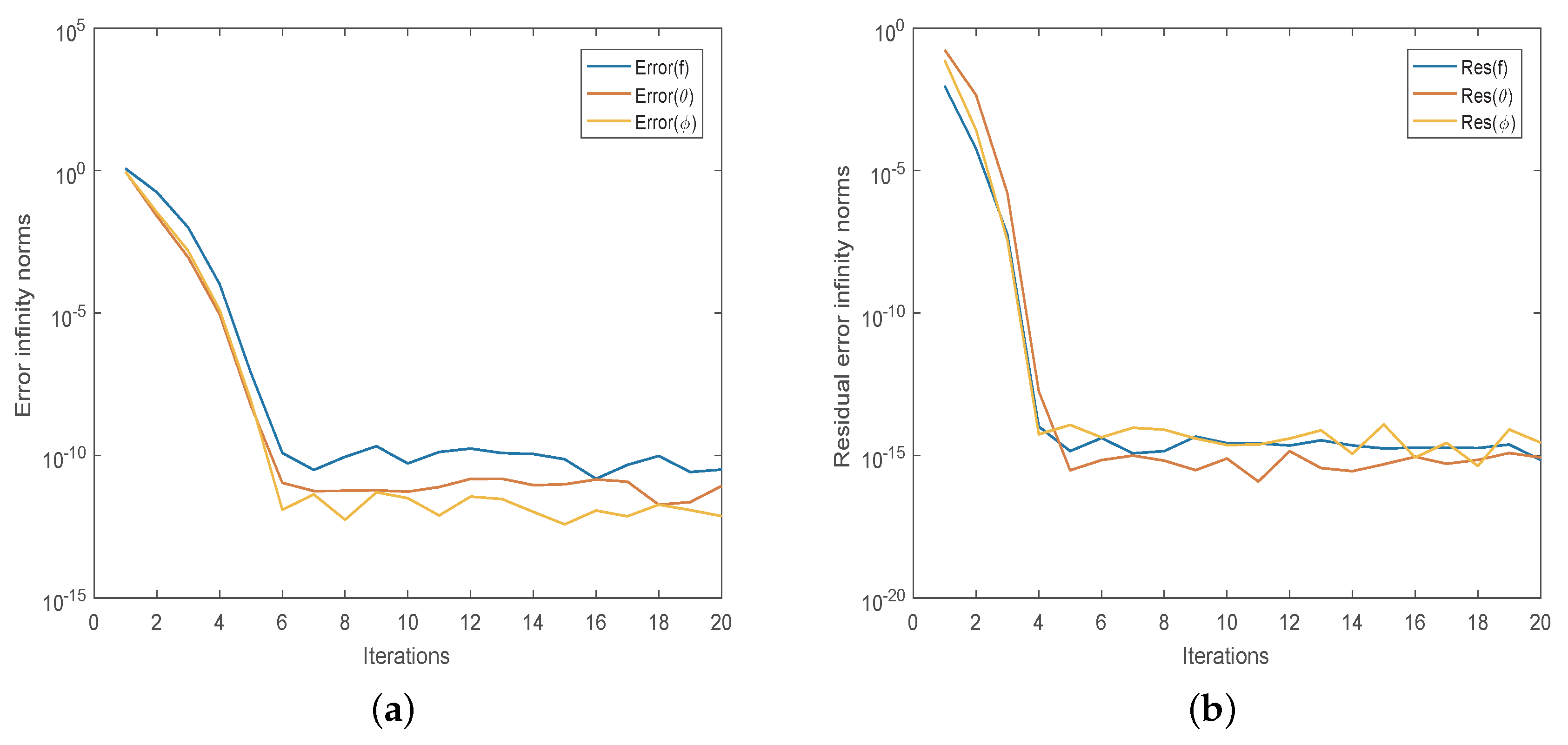
3. Method of Solution

In this section we present a spectral method based on a quasi-linearization method called the spectral quasi-linearization method (SQLM), Motsa et al. [42]. The SQLM combines two methods, the quasi-linearization method (QLM) and a Chebyshev spectral collocation method (CSCM). The QLM, a Newton-Raphson based quasi-linearzation method which was introduced by Bellman and Kalaba [43], is used to linearize the governing non-linear equations. The CSCM is used to integrate the resulting iterative sequence of linear differential equations.

3.1. Quasi-Linearization

With reference to Equations (10)–(12), we derive the quasi-linearization formula by considering a system of differential equations
Λ p [ ζ 1 , ζ 2 , ζ 3 ] = 0 , p = 1 , 2 , 3 ,
where Λ p ( p = 1 , 2 , 3 ) are non-linear operators, ζ 1 = { f , f , f , f } , ζ 2 = { θ , θ , θ } and ζ 3 = { ϕ , ϕ , ϕ } . Denote f s , θ s , ϕ s and f s + 1 , θ s + 1 , ϕ s + 1 be the solutions of Equation (17) at the previous and the current iteration levels, respectively. Assuming the difference between the solution at the previous and the current iteration levels and its derivatives is small enough, linear Taylor series expansion of Equation (17) about some previous solution, upon simplification yields
ζ s + 1 1 · f Λ p [ f s , θ s , ϕ s ] + ζ s + 1 2 · θ Λ p [ f s , θ s , ϕ s ] + ζ s + 1 3 · ϕ Λ p [ f s , θ s , ϕ s ] = ζ s 1 · f Λ p [ f s , θ s , ϕ s ] + ζ s 2 · θ Λ p [ f s , θ s , ϕ s ] + ζ s 3 · ϕ Λ p [ f s , θ s , ϕ s ] Λ p [ f s , θ s , ϕ s ] , s = 0 , 1 , 2 , ,
where f = { f , f , f , f } , θ = { θ , θ , θ } and ϕ = { ϕ , ϕ , ϕ } . Applying the formula Equation (18) to the system Equations (10)–(12) results in an iterative sequence of linear equations
a 0 , s f s + 1 + a 1 , s f s + 1 + a 2 , s f s + 1 + a 3 , s f s + 1 + a 4 , s θ s + 1 + a 5 , s ϕ s + 1 = R 1 , s ,
b 0 , s θ s + 1 + b 1 , s θ s + 1 + b 2 , s θ s + 1 + b 3 , s f s + 1 + b 4 , s f s + 1 + b 5 , s f s + 1 = R 2 , s ,
c 0 , s ϕ s + 1 + c 1 , s ϕ s + 1 + c 2 , s ϕ s + 1 + c 3 , s f s + 1 + c 4 , s f s + 1 = R 3 , s ,
where the variable coefficients are given by
a 0 , s = 1 + 2 W e f s , a 1 , s = 2 W e f s + f s η 2 S , a 2 , s = 2 f s S M 2 , a 3 , s = f s , a 4 , s = λ 1 , a 5 , s = λ 2 , b 0 , s = 1 P r ( 1 + 4 3 R ) , b 1 , s = f s η 2 S , b 2 , s = 2 S f s , b 3 , s = 2 E c f s + 3 E c W e ( f s ) 2 , b 4 , s = 2 M 2 E c ( f s E 1 ) θ s , b 5 , s = θ s , c 0 , s = 1 S c , c 1 , s = f s η 2 S , c 2 , s = 2 S f s γ , c 3 , s = ϕ s , c 4 , s = ϕ s .
The terms on the right are defined as follows:
R 1 , s = 2 W e f s f s + f s f s ( f s ) 2 M 2 E 1 , R 2 , s = f s θ s f s θ s + E c ( f s ) 2 + 2 E c W e ( f s ) 3 + M 2 E c [ ( f s ) 2 E 1 2 ] , R 3 , s = f s ϕ s ϕ s f s .

3.2. Chebyshev Differentiation

We approximate the solutions of Equations (10)–(12) by functions of the form
f ( η ) = k = 0 N f ( η k ) L k ( η ) , θ ( η ) = k = 0 N θ ( η k ) L k ( η ) , ϕ ( η ) = k = 0 N ϕ ( η k ) L k ( η ) ,
where
L k ( η ) = j = 0 k j N η η j η k η j ,
is the Lagrange interpolating polynomial. For convenience in the application of the collocation method, we transform the semi-infinite physical domain [ 0 , ) in the η -direction to [ 1 , 1 ] in the x-direction using the linear transformation η = l 2 ( 1 + x ) . ( l is a number chosen to be large enough that boundary conditions at ∞ hold). Evaluating the approximating functions (22) and their derivatives at Chebyshev-Gauss-Lobatto points
{ η i } = cos π i N , i = 0 , 1 , , N ,
gives
d f d η | η = η i = k = 0 N f ( η k ) d d η L k ( η i ) = D F , d n f d η n | η = η i = D n F ,
where D = 2 l D , D is an ( N + 1 ) × ( N + 1 ) Chebyshev differentiation matrix, Trefethen [44], F = [ f ( η 0 ) , f ( η 1 ) , , f ( η N 1 ) , f ( η N ) ] T and T denotes matrix transpose. θ and ϕ have similar expressions for derivatives. Evaluating Equations (19)–(21) at the collocation points and approximating derivatives with Chebyshev derivatives gives, in vector matrix form, the system
A 11 A 12 A 31 A 21 A 22 A 23 A 31 A 32 A 33 F s + 1 Φ s + 1 Θ s + 1 = R 1 , s R 2 , s R 3 , s ,
where
A 11 = a 0 , s D 3 + a 1 , s D 2 + a 2 , s D + a 3 , s , A 12 = a 4 , s , A 13 = a 5 , s A 21 = b 3 , s D 2 + b 4 , s D + b 5 , s , A 22 = b 0 , s D 2 + b 1 , s D + b 2 , s . A 23 = 0 , A 31 = c 3 , s D + c 4 , s , A 32 = 0 , A 33 = c 0 , s D 2 + c 1 , s D + c 2 , s , R k , s = { R k , s ( η 0 ) , R k , s ( η 1 ) , , R k , s ( η N 1 ) , R k , s ( η N ) } T , ( k = 1 , 2 , 3 ) .

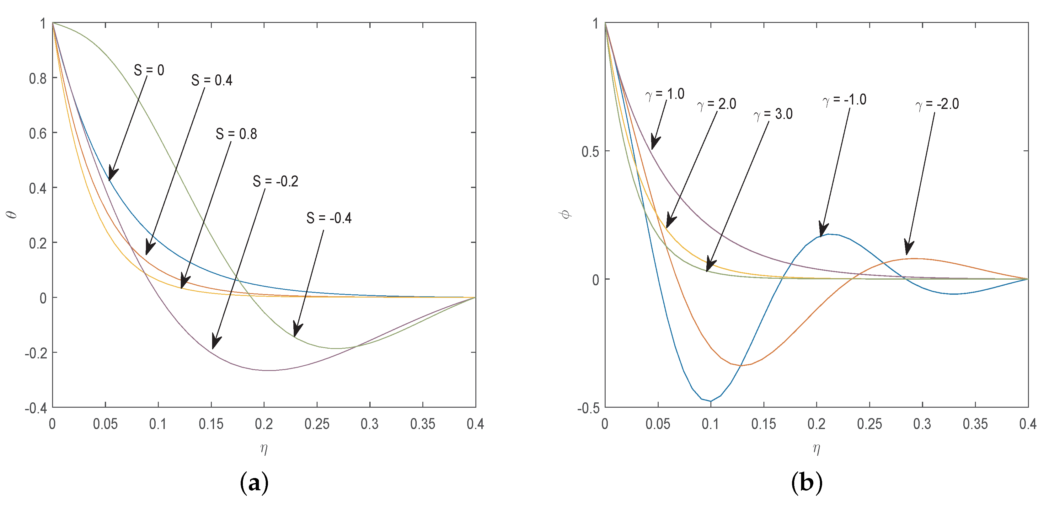
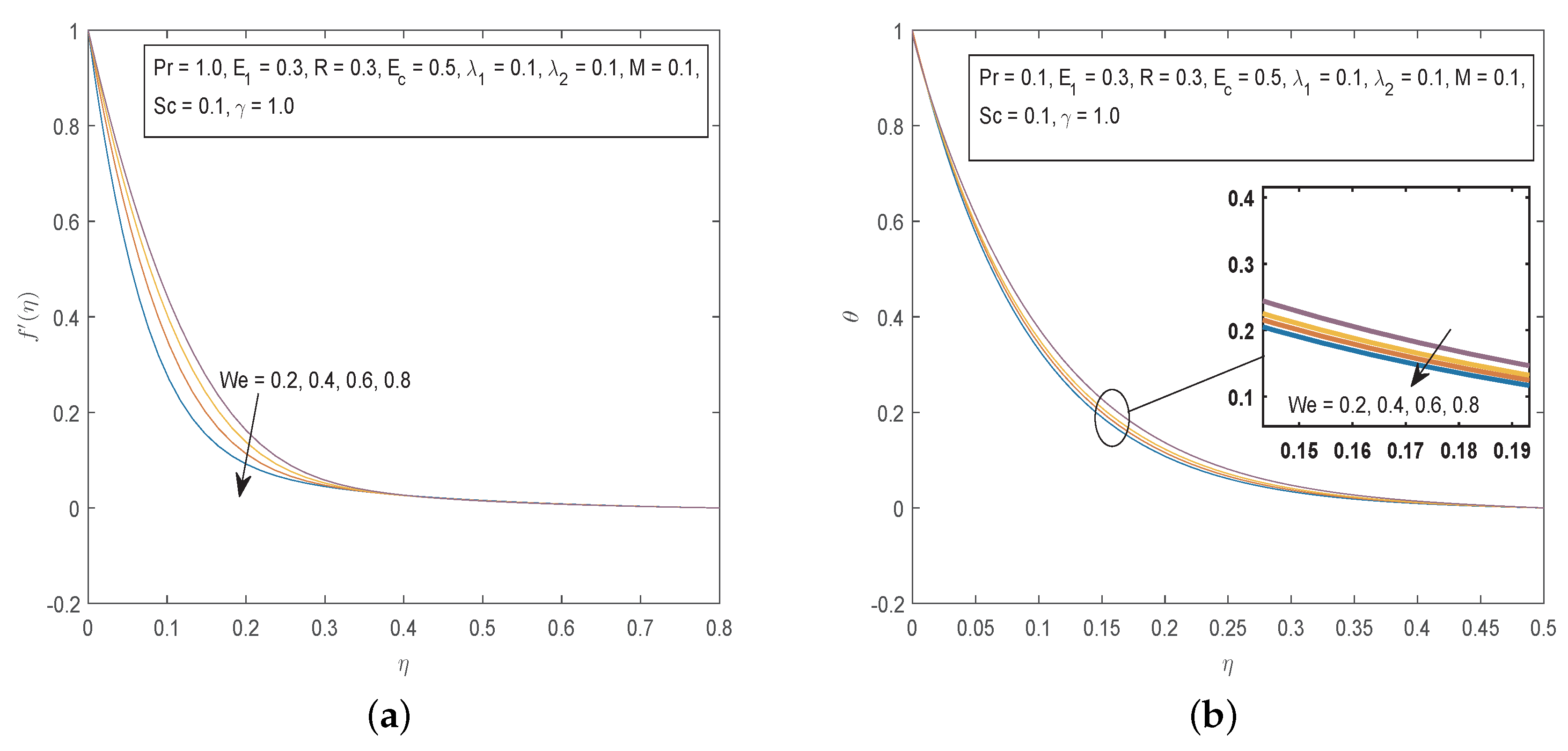
4. Results and Discussions

The spectral quasi-linearization method was used to generate the results to be discussed in this section. All the numerical results were obtained using MATLAB 2016. For all the computations, the default parameters considered, unless otherwise stated, are N = 60 , P r = 1 . 0 , W e = 0 . 1 , E 1 = 0 . 3 , E c = 0 . 5 , R = 0 . 3 , λ 1 = 0 . 1 , λ 2 = 0 . 1 , S c = 0 . 1 , γ = 1 . 0 and f w = 0 . 3 .
The error infinity norms defined by
Error ( f ) = max 0 i N | | F s + 1 , i F s , i | | , Error ( θ ) = max 0 i N | | Θ s + 1 , i Θ s , i | | , Error ( ϕ ) = max 0 i N | | Φ s + 1 , i Φ s , i | | ,
are used to confirm the convergence of the SQLM solution. The accuracy of the SQLM is tested using the residual error infinity norms defined as follows:
| | R e s ( f ) | | = | | ( 1 + 2 W e f ) f + f f ( f ) 2 S f + η 2 f + M 2 ( E 1 f ) + λ 1 θ + λ 2 ϕ | | , | | R e s ( θ ) | | = | | 1 P r 1 + 4 R 3 θ + f θ S η 2 θ ( 2 S + f ) θ + E c ( ( f ) 2 + W e ( f ) 3 ) + M 2 E c ( f E 1 ) 2 | | , | | R e s ( ϕ ) | | = | | 1 S c ϕ + f S η 2 ϕ + ( 2 S f γ ) ϕ | | .
Figure 2 shows the convergence and accuracy of the SQLM. We note that an increase in the number of iterations results in a decrease of the error infinity norm and method converges after six iterations. Also, the decrease in residual error infinity norms against the number of iterations confirms the accuracy of the numerical method. The SQLM achieves an accuracy of order 10 15 after five iterations, showing that the method is highly accurate.
Figure 3 shows the sensitivity of temperature and concentration profiles with the unsteadiness parameter S and the chemical reaction parameter γ , respectively. It is shown that for values of S 0 , the temperature profiles show the expected trend, satisfying boundary conditions (13) and (14). For values of S < 0 , the profiles behave unexpectedly. Similarly, the concentration profiles show the desired pattern for values of γ > 0 , satisfying the underlying boundary conditions (13) and (14). We remark that these chaotic and high sensitivity behaviour happen when the method has not yet reached the convergence stage. Once convergence has been reached, the behaviour becomes normal as expected. This can clearly be observed in subsequent figures.
The effects of the emerging physical parameters of importance in this study on the fluid velocity, temperature and concentration fields are shown in Figure 4, Figure 5, Figure 6, Figure 7, Figure 8, Figure 9, Figure 10, Figure 11 and Figure 12. The effects of the Weissenberg number W e on the fluid velocity f ( η ) and the fluid temperature θ ( η ) is shown in Figure 4. It is noted that the velocity profiles are decreasing functions of W e . The Weissenberg number gives the ratio of relaxation time to specific process time. Increasing W e translates to a decrease in the specific process time which in turn will cause a decrease in the velocity component as well as the boundary layer thickness. Increasing the values of W e results in a decrease in the fluid temperature profiles.
Figure 5 shows the graphs of the dimensionless concentration profiles for different values of the Schmidt number S c and the chemical reaction parameter γ . We can observe that increasing S c results in a decrease in the fluid concentration. Physically, since S c is dependent on fluid mass diffusivity, high values of S c correspond to a decrease in mass diffusion hence the concentration profile is reduced. The concentration profiles are also decreased by increasing the chemical reaction. This is due to the fact that a higher chemical reaction results in a decrease in chemical molecular diffusivity leading to a reduction in mass diffusion. The decrease in concentration of the diffusing species will result in the thinning of the concentration boundary layer.
The influence of the magnetic field parameter on the fluid velocity and temperature is presented in Figure 6. We notice that increasing the values of the magnetic field parameter has an effect of slowing down the fluid motion. Physically, the presence of a magnetic field creates a drag-like force called the Lorentz force that opposes the motion of the fluid and resists the velocity of the fluid. The variation of the magnetic parameter M on θ ( η ) shows an opposite trend. We observe that the temperature profiles increase as the magnetic field parameter increases. This is because, as mentioned earlier on, an increase in M reduces the magnitude of the velocity profiles in the boundary layer, hence will cause a rise in the temperature in the boundary layer.
Figure 7 shows that an increase in the magnetic parameter causes an increase in the concentration field. We noted earlier that increasing the magnetic parameter reduces the velocity profiles in the boundary which in turn induces the diffusion of the particles in the boundary layer. The increment of the thermal buoyancy parameter λ 1 causes a decline in the fluid concentration.
The effects of the thermal radiation parameter R and the Prandtl number P r on the temperature profiles are depicted on Figure 8. We can see that the fluid temperature increases with increasing values of the thermal radiation parameter R. P r is inversely proportional to thermal diffusivity. Increasing the values of P r causes a decrease in the temperature field. Physically, high values of P r are associated with low thermal conductivity which reduces conduction and hence the thermal boundary layer resulting in a decrease in fluid temperature.
As shown in Figure 9, the temperature profiles decrease with the increase in the values of the buoyancy parameters λ 1 and λ 2 . It is clearly noted that an increase in thermal buoyancy parameter causes a decrease in the thermal boundary layer thickness and consequently the fluid temperature decreases due to the buoyancy effect.
From Figure 10 it can be seen that the velocity and temperature profiles decrease as the unsteadiness parameter S increases. The effect of E 1 on the fluid velocity is the opposite of that of S. Figure 11 depicts that increasing the values of the local electric parameter E 1 results in an increase in both the velocity and concentration fields. Figure 12 shows the effects of increasing the values of Eckert number E c on the temperature profiles and λ 1 on velocity profiles. The Eckert number characterize the influence of self heating of a fluid as a consequence of dissipation effects. Viscous dissipation due to internal friction of the fluid will cause an increase in the fluid temperature. Increasing the value of the thermal buoyancy parameter λ 1 leads to an increase in the velocity profiles.
The examination of influence of the emerging parameters on the physical quantities of engineering importance, namely the skin friction coefficient, Nusselt number and Sherwood number is depicted in Table 1, Table 2 and Table 3. Table 1 shows that the skin friction increases as the values of S, M, P r , γ , S c and E c are increased. The opposite trend is observed for the parameters E 1 , λ 1 , R and W e . In Table 2, we can see that the heat transfer rate increased by the increasing values of S, E 1 , λ 1 , λ 2 , P r and R. The heat transfer rate is depressed as the the values of M, γ , S c and E c . Table 3 shows that the coefficient of the Sherwood number is an increasing function of E 1 , λ 1 , λ 2 , γ , S c , R and E c and a decreasing function of S, M, P r and W e .

5. Conclusions

A Williamson fluid is characteristic of a non-Newtonian fluid model with shear thinning property. The model constitute a coupled system of nonlinear partial differential equations. The transformed coupled system of dimensionless non-linear ordinary differential equations was successfully solved using the spectral quas-linearization method. The use of error infinity norms and residual error infinity norms confirmed that the numerical technique is convergent and accurate, respectively. In this present study, we numerically analyzed the effects of viscous dissipation, thermal radiation, chemical reaction and uniform magnetic field on the unsteady boundary layer flow of an electrically conducting Williamson fluid over a stretching sheet. We conclude the most important findings of the study as follows:
  • The SQLM is a very efficient and accurate method.
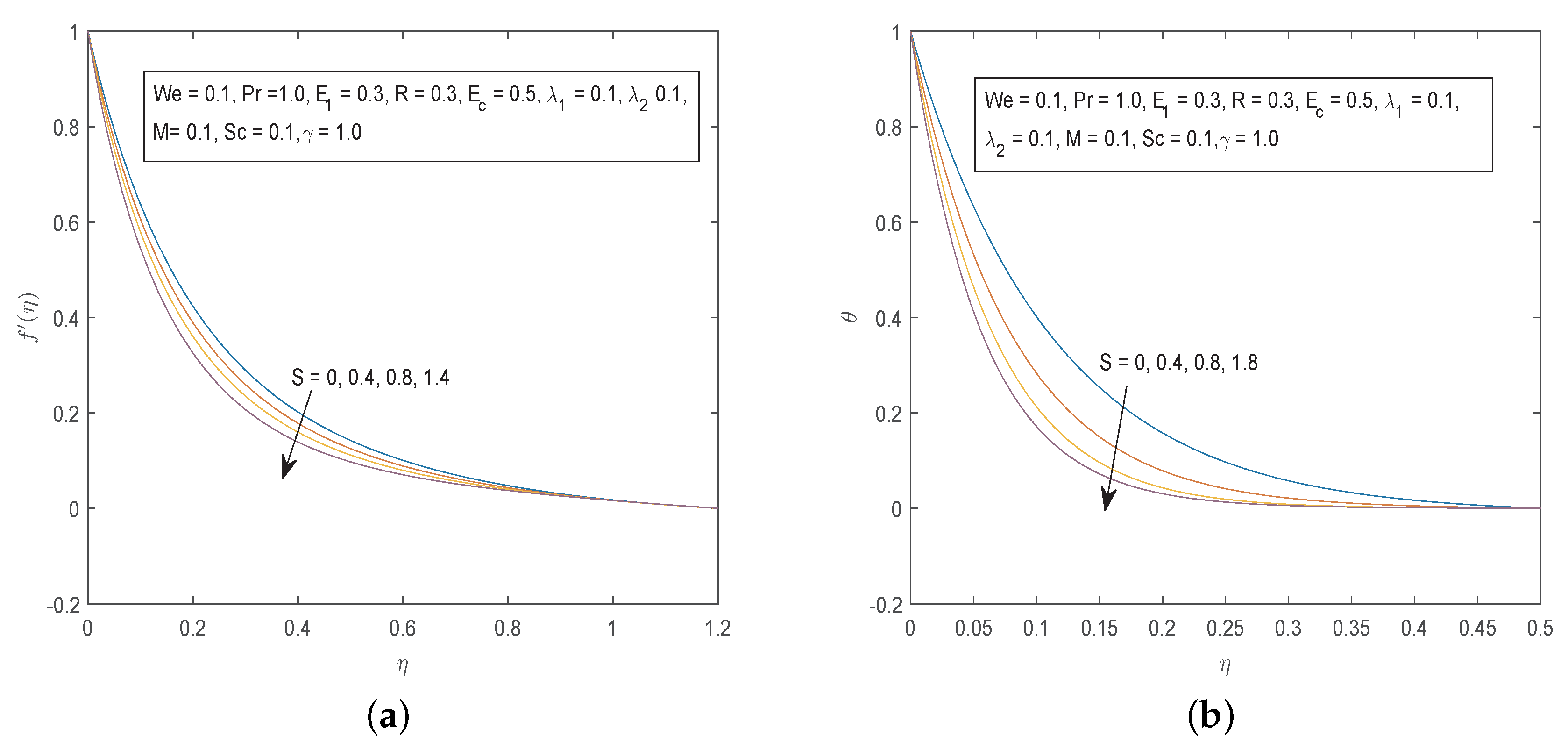
  • The fluid velocity and the momentum boundary layer decrease with respective, increases in the Williamson parameter, unsteadiness parameter, magnetic parameter, Eckert number as well as the Prandtl and Schmidt numbers.
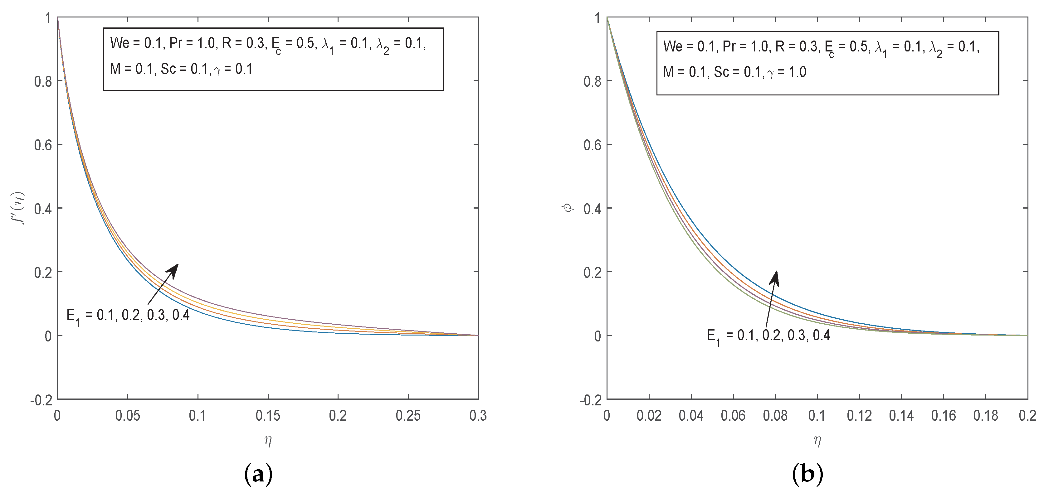
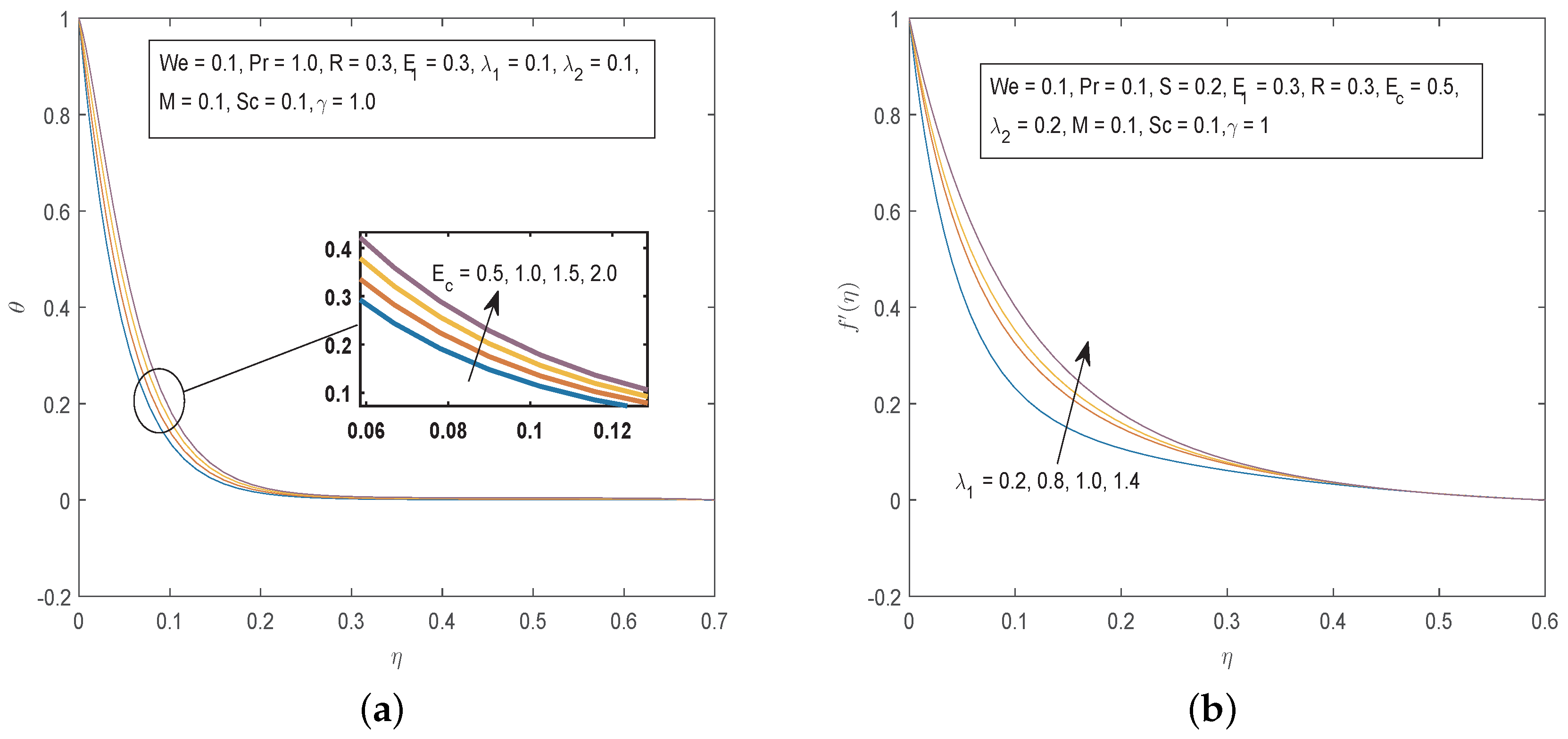
  • The fluid velocity and the momentum boundary layer increase with increasing values of the electric parameter, buoyancy parameters, thermal radiation and chemical reaction parameter.
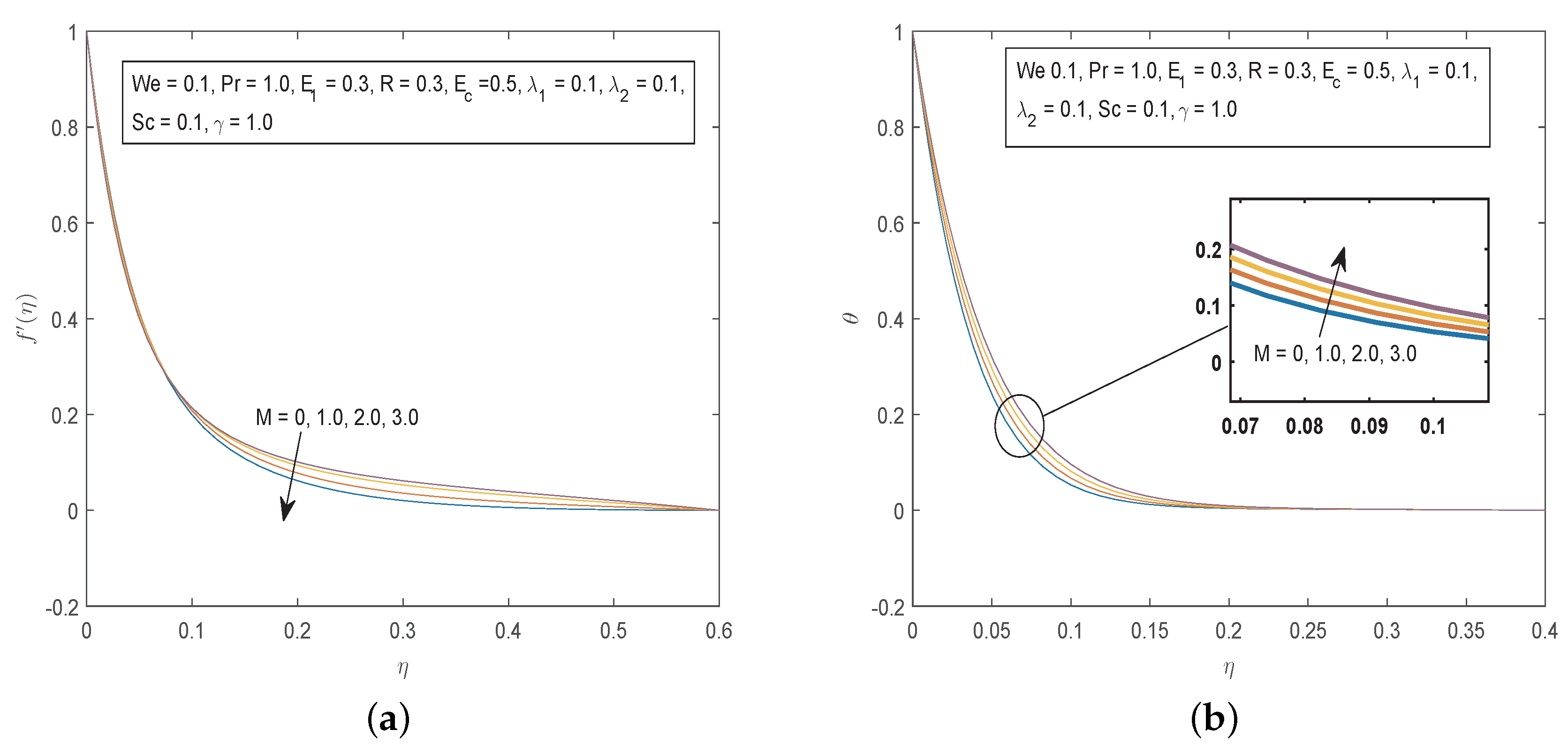
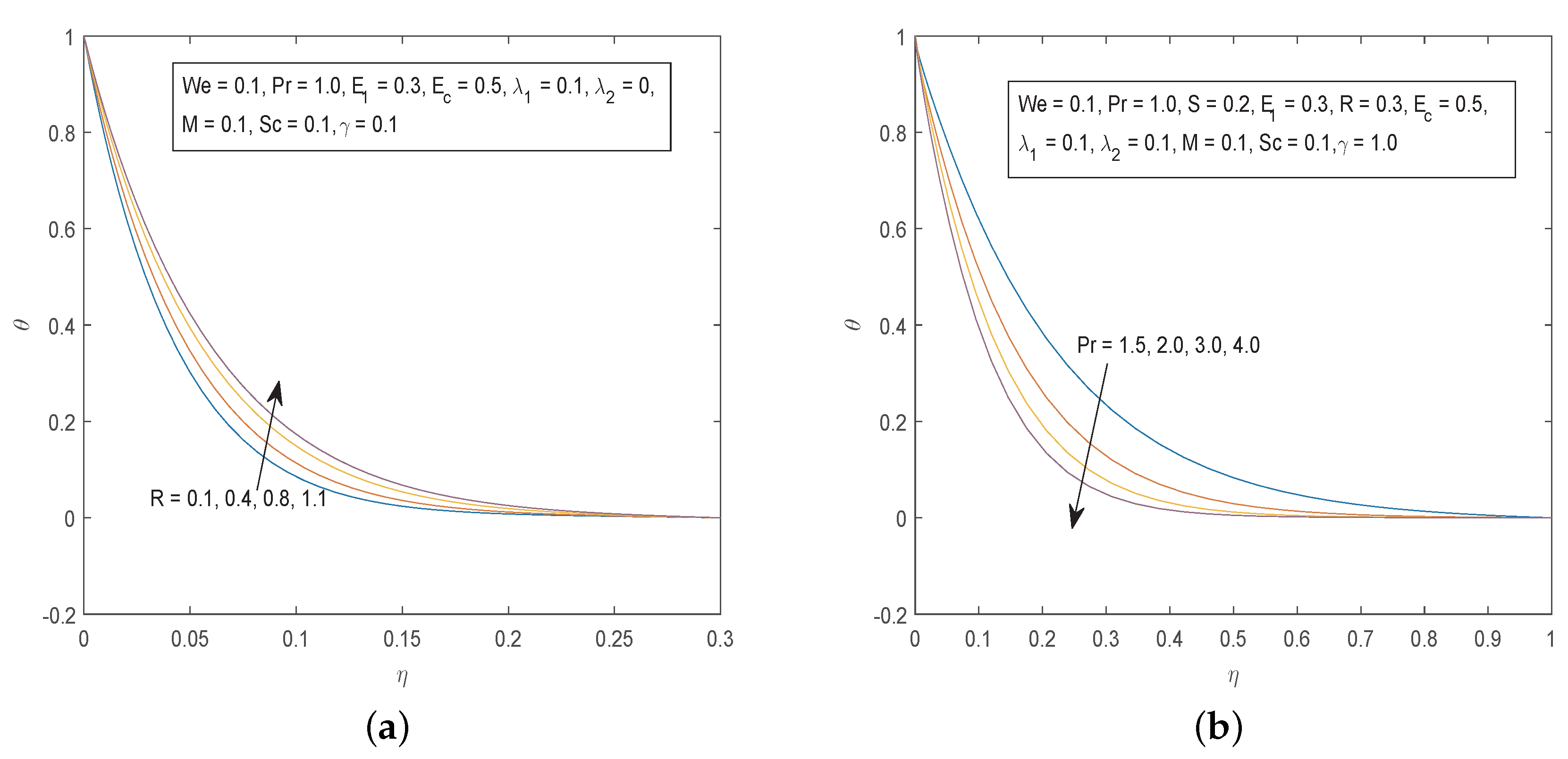
  • The fluid temperature increases as the values of the magnetic parameter, thermal radiation parameter, electrical parameter and Eckert number increase.
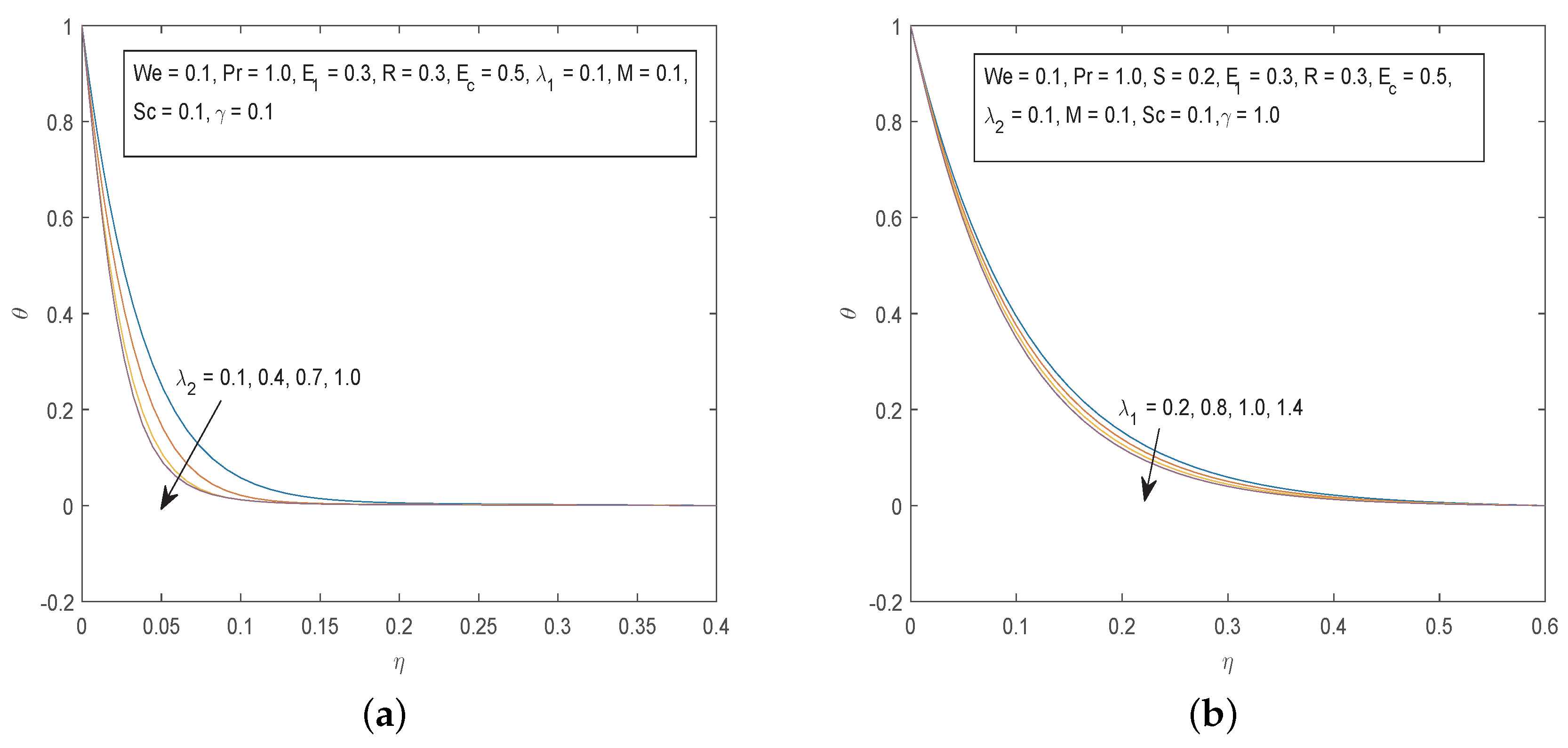
  • The fluid temperature is a decreasing function of the buoyancy parameter, Prandtl number, unsteadiness parameter as well as the Williamson number.
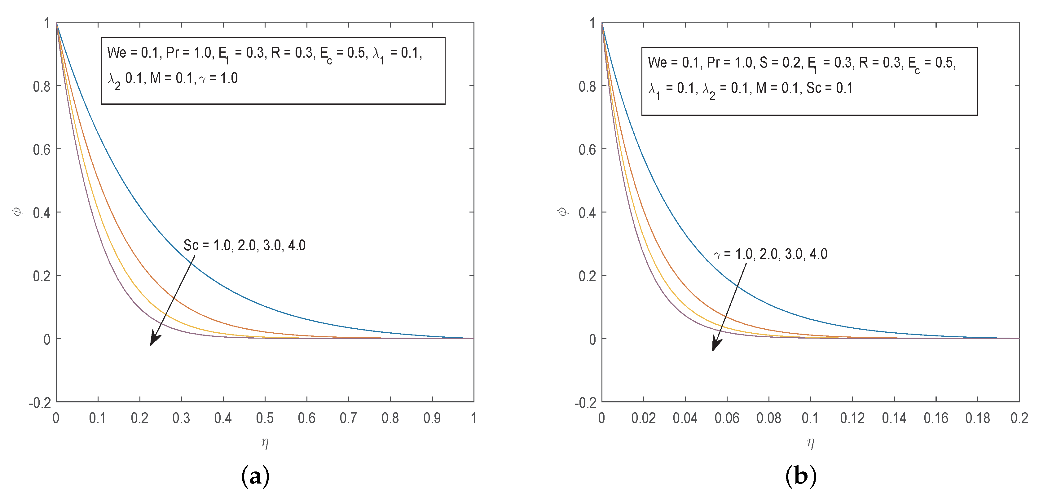
  • The stretching parameter, chemical reaction parameter, suction, Schmidt number, buoyancy parameters and the Williamson number were found to reduce the concentration profiles.
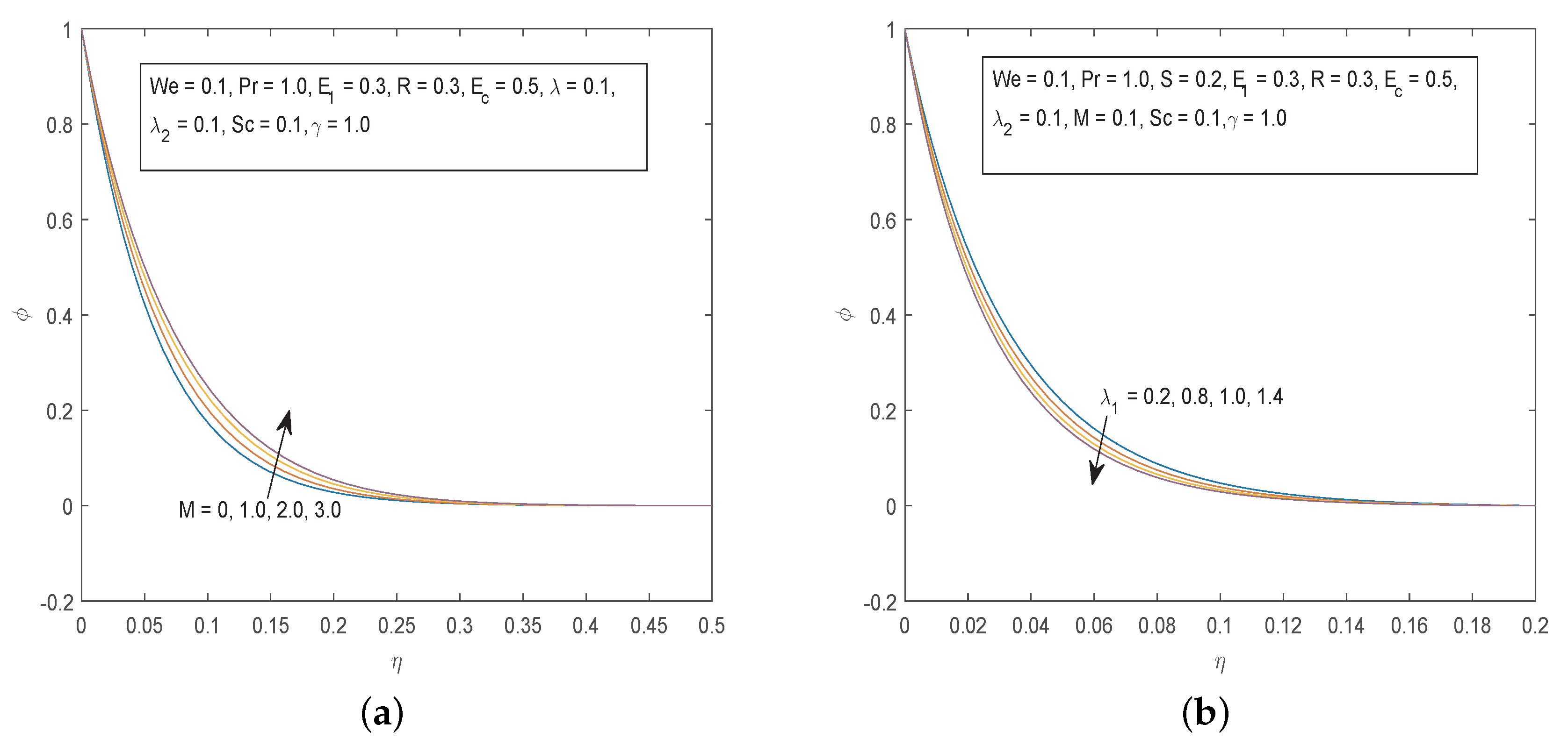
  • The concentration was observed to be increasing as the values of the magnetic parameter, injection and Eckert number increase.
  • The skin friction increases with the increase of the unsteadiness parameter, magnetic parameter, Prandtl number, Schmidt number, chemical reaction parameter, and thermal radiation parameter.
  • However, the skin friction decreases with increasing values of the Eckert number, buoyancy parameters, thermal radiation and the Williamson number.
  • The wall temperature gradient decreases with the increasing values of the Williamson number, suction, magnetic parameter, chemical reaction parameter, Schmidt number and Eckert number.
  • The study observed that the Nusselt number increases with the increase of the unsteadiness parameter, electric parameter, buoyancy parameters, Prandtl number, thermal radiation parameter, and the Williamson number.
  • The unsteadiness parameter, magnetic parameter, the Prandtl number and the Williamson number cause the wall concentration gradient to decrease.
  • Lastly, the Sherwood number increases as the values of the electric parameter, buoyancy parameters, chemical reaction, Schmidt number, thermal radiation and Eckert number increase.
The joy of the current paper lies in the accuracy and fast convergence of the used numerical technique. Therefore, the method may also be valid for other complex nonlinear boundary value problems even with chaotic behaviour. We recommend that these results can be used as a standard example for other applications in engineering and applied sciences.

Author Contributions

Conceptualization, S.S.; methodology, S.S. and H.M.; generation of results, H.M.; validation, S.S. and H.M.; formal analysis, S.S. and H.M.; resources, S.M.; writing—original draft preparation, S.S. and H.M.; writing—review and editing, S.S.; project administration, S.S.; funding acquisition, S.S. All authors have read and agreed to the published version of the manuscript.

Funding

This research was funded by the University of Venda through funding my research visit as well as the publication charges.

Acknowledgments

The assistance from the honourable editor and the anonymous reviewers in the preparation of this article is highly acknowledged.

Conflicts of Interest

The authors declare no conflict of interest. The funders had no role in the design of the study; in the collection, analyses, or interpretation of data; in the writing of the manuscript, or in the decision to publish the results.

References

  1. Kahshan, M.; Lu, D.; Rahimi-Gorji, M. Hydrodynamical study of flow in a permeable channel: Application to flat plate dialyzer. Int. J. Hydrogen Energy 2019, 44, 17041–17047. [Google Scholar] [CrossRef]
  2. Hussanan, A.; Salleh, M.Z.; Tahar, R.; Khan, I. Unsteady Boundary Layer Flow and Heat Transfer of a Casson Fluid past an Oscillating Vertical Plate with Newtonian Heating. PLoS ONE 2014, 9, e108763. [Google Scholar] [CrossRef] [PubMed] [Green Version]
  3. Cioranescu, D.; Girault, V.; Rajagopal, K.R. Mechanics and Mathematics of Fluids of the Differential Type: Advances in Mechanics and Mathematics; Springer International Publishing: Cham, Switzerland, 2016. [Google Scholar] [CrossRef]
  4. Miccichè, C.C.; Arrabito, G.; Amato, F.; Buscarino, G.; Agnello, S.; Pignataro, B. Inkjet printing Ag nanoparticles for SERS hot spots. Anal. Methods 2018, 10, 3215–3223. [Google Scholar] [CrossRef]
  5. Dybowska-Sarapuk, L.; Kielbasinski, K.; Araźna, A.; Futera, K.; Skalski, A.; Janczak, D.; Sloma, M.; Jakubowska, M. Efficient Inkjet Printing of Graphene-Based Elements: Influence of Dispersing Agent on Ink Viscosity. Nanomaterials 2018, 8, 602. [Google Scholar] [CrossRef] [PubMed] [Green Version]
  6. Mozaffari, S.; Tchoukov, P.; Mozaffari, A.; Atias, J.; Czarnecki, J.; Nazemifard, N. Capillary driven flow in nanochannels—Application to heavy oil rheology studies. Colloids Surf. A Physicochem. Eng. Asp. 2017, 513, 178–187. [Google Scholar] [CrossRef]
  7. Mozaffari, S.; Li, W.; Dixit, M.; Seifert, S.; Lee, B.; Kovarik, L.; Mpourmpakis, G.; Karim, A.M.; Seifert, S. The role of nanoparticle size and ligand coverage in size focusing of colloidal metal nanoparticles. Nanoscale Adv. 2019, 1, 4052–4066. [Google Scholar] [CrossRef] [Green Version]
  8. Darjani, S.; Koplik, J.; Banerjee, S.; Pauchard, V. Liquid-hexatic-solid phase transition of a hard-core lattice gas with third neighbor exclusion. J. Chem. Phys. 2019, 151, 104702. [Google Scholar] [CrossRef]
  9. Xing, X.; Pei, J.; Shen, C.; Li, R.; Zhang, J.; Huang, J.; Hu, D. Performance and Reinforcement Mechanism of Modified Asphalt Binders with Nano-Particles, Whiskers, and Fibers. Appl. Sci. 2019, 9, 2995. [Google Scholar] [CrossRef] [Green Version]
  10. Elgazery, N.S. Flow of non-Newtonian magneto-fluid with gold and alumina nanoparticles through a non-Darcian porous medium. J. Egypt. Math. Soc. 2019, 27, 1–25. [Google Scholar] [CrossRef] [Green Version]
  11. Hsiao, K.-L. To promote radiation electrical MHD activation energy thermal extrusion manufacturing system efficiency by using Carreau-Nanofluid with parameters control method. Energy 2017, 130, 486–499. [Google Scholar] [CrossRef]
  12. Seikh, A.; Akinshilo, A.; Taheri, M.H.; Rahimi-Gorji, M.; Alharthi, N.H.; Khan, I.; Khan, A.R. Influence of the nanoparticles and uniform magnetic fieldon the slip blood flows in arterial vessels. Phys. Scr. 2019, 94, 125218. [Google Scholar] [CrossRef]
  13. Abdal, S.; Ali, B.; Younas, S.; Ali, L.; Mariam, A. Thermo-Diffusion and Multislip Effects on MHD Mixed Convection Unsteady Flow of Micropolar Nanofluid over a Shrinking/Stretching Sheet with Radiation in the Presence of Heat Source. Symmetry 2019, 12, 49. [Google Scholar] [CrossRef] [Green Version]
  14. Adesanya, S.O.; Souayeh, B.; Rahimi-Gorji, M.; Khan, M.; Adeyemi, O.G. Heat irreversibiility analysis for a couple stress fluid flow in an inclined channel with isothermal boundaries. J. Taiwan Inst. Chem. Eng. 2019, 101, 251–258. [Google Scholar] [CrossRef]
  15. Williamson, R.V. The Flow of Pseudoplastic Materials. Ind. Eng. Chem. 1929, 21, 1108–1111. [Google Scholar] [CrossRef]
  16. Nadeem, S.; Hussain, S.T.; Lee, C. Flow of a Williamson fluid over a stretching sheet. Braz. J. Chem. Eng. 2013, 30, 619–625. [Google Scholar] [CrossRef] [Green Version]
  17. Nadeem, S.; Hussain, S.T. Heat transfer analysis of Williamson fluid over exponentially stretching surface. Appl. Math. Mech. 2014, 35, 489–502. [Google Scholar] [CrossRef]
  18. Khan, W.; Gul, T.; Idrees, M.; Islam, S.; Khan, I.; Dennis, L. Thin Film Williamson Nanofluid Flow with Varying Viscosity and Thermal Conductivity on a Time-Dependent Stretching Sheet. Appl. Sci. 2016, 6, 334. [Google Scholar] [CrossRef] [Green Version]
  19. Khan, M.I.; Alsaedi, A.; Qayyum, S.; Hayat, T. Consequences of Binary Chemically Reactive Flow Configuration of Williamson Fluid with Entropy Optimization and Activation Energy. Int. J. Thermophys. 2019, 40, 94. [Google Scholar] [CrossRef]
  20. Monica, M.; Sucharitha, J.; Kumar, C.K. Stagnation Point Flow of a Williamson Fluid over a Nonlinearly Stretching Sheet with Thermal Radiation. Am. Chem. Sci. J. 2016, 13, 1–8. [Google Scholar] [CrossRef]
  21. Malik, M.; Bibi, M.; Khan, F.; Salahuddin, T. Numerical solution of Williamson fluid flow past a stretching cylinder and heat transfer with variable thermal conductivity and heat generation/absorption. AIP Adv. 2016, 6, 35101. [Google Scholar] [CrossRef] [Green Version]
  22. Mabood, F.; Ibrahim, S.; Lorenzini, G.; Lorenzin, E. Radiation effects on Williamson nanofluid flow over a heated surface with magnetohydrodynamics. Int. J. Heat Technol. 2017, 35, 196–204. [Google Scholar] [CrossRef]
  23. Dawar, A.; Shah, Z.; Islam, S.; Khan, W.; Idrees, M. An optimal analysis for Darcy–Forchheimer three-dimensional Williamson nanofluid flow over a stretching surface with convective conditions. Adv. Mech. Eng. 2019, 11, 168781401983351. [Google Scholar] [CrossRef] [Green Version]
  24. Kumar, K.G.; Rudraswamy, N.; Gireesha, B.; Manjunatha, S. Non linear thermal radiation effect on Williamson fluid with particle-liquid suspension past a stretching surface. Results Phys. 2017, 7, 3196–3202. [Google Scholar] [CrossRef]
  25. Shateyi, S.; Mabood, F.; Lorenzini, G. Casson fluid flow: Free convective heat and mass transfer over an unsteady permeable stretching surface considering viscous dissipation. J. Eng. Thermophys. 2017, 26, 39–52. [Google Scholar] [CrossRef]
  26. Hayat, T.; Shafiq, A.; Alsaedi, A. Hydromagnetic boundary layer flow of Williamson fluid in the presence of thermal radiation and Ohmic dissipation. Alex. Eng. J. 2016, 55, 2229–2240. [Google Scholar] [CrossRef] [Green Version]
  27. Khan, M.; Malik, M.; Salahuddin, T.; Rehman, K.; Naseer, M.; Khan, I. MHD flow of Williamson nanofluid over a cone and plate with chemically reactive species. J. Mol. Liq. 2017, 231, 580–588. [Google Scholar] [CrossRef]
  28. Panezai, A.; Rehman, A.; Sheikh, N.; Iqbal, S.; Ahmed, I.; Iqbal, M.; Zulfiqar, M. Mixed Convective Magnetohydrodynamic Heat Transfer Flow of Williamson Fluid Over a Porous Wedge. Am. J. Math. Comput. Model. 2019, 4, 66–73. [Google Scholar] [CrossRef] [Green Version]
  29. Huang, C.-J.; Hsu, H.-P.; Ay, H.-C. Influence of mhd on free convection of non-newtonian fluids over a vertical permeable plate in porous media with internal heat generation. Front. Heat Mass Transf. 2019, 13, 14. [Google Scholar] [CrossRef]
  30. Kebede, T.; Haile, E.; Awgichew, G.; Walelign, T. Heat and Mass Transfer in Unsteady Boundary Layer Flow of Williamson Nanofluids. J. Appl. Math. 2020, 2020, 1–13. [Google Scholar] [CrossRef]
  31. Reddy, C.S.; Naikoti, K.; Rashidi, M.M. MHD flow and heat transfer characteristics of Williamson nanofluid over a stretching sheet with variable thickness and variable thermal conductivity. Trans. A. Razmadze Math. Inst. 2017, 171, 195–211. [Google Scholar] [CrossRef]
  32. Megahed, A.M. Williamson fluid flow due to a nonlinearly stretching sheet with viscous dissipation and thermal radiation. J. Egypt. Math. Soc. 2019, 27, 1–10. [Google Scholar] [CrossRef] [Green Version]
  33. Sakiadis, B.C. Boundary-layer behavior on continuous solid surfaces: I. Boundary-layer equations for two-dimensional and axisymmetric flow. AIChE J. 1961, 7, 26–28. [Google Scholar] [CrossRef]
  34. Crane, L.J. Flow past a stretching plate. Z. Angew. Math. Phys. (ZAMP) 1970, 21, 645–647. [Google Scholar] [CrossRef]
  35. Hsiao, K.-L. Stagnation electrical MHD nanofluid mixed convection with slip boundary on a stretching sheet. Appl. Therm. Eng. 2016, 98, 850–861. [Google Scholar] [CrossRef]
  36. Hsiao, K.-L. Micropolar nanofluid flow with MHD and viscous dissipation effects towards a stretching sheet with multimedia feature. Int. J. Heat Mass Transf. 2017, 112, 983–990. [Google Scholar] [CrossRef]
  37. Shateyi, S. Numerical analysis of cattaneo-christov heat flux model and mass transfer mhd mixed convection flow of a maxwell fluid over a stretching sheet with soret effects. JP J. Heat Mass Transf. 2018, 15, 675–691. [Google Scholar] [CrossRef]
  38. Choudhary, S.; Sharma, P.; Makinde, O. MHD slip flow and heat transfer over an exponentially stretching permeable sheet embedded in a porous medium with heat source. Front. Heat Mass Transf. 2017, 9. [Google Scholar] [CrossRef] [Green Version]
  39. Shamshuddin, M.D.; Chamkha, A.; Thumma, T.; Raju, M. Computation of unsteady mhd mixed convective heat and mass transfer in dissipative reactive micropolar flow considering sorte and dufour effects. Front. Heat Mass Transf. 2018, 10, 4. [Google Scholar] [CrossRef] [Green Version]
  40. Nagalakshm, P.; Vijaya, N. MHD flow of carreau nanofluid explored using cnt over a nonlinear stretched sheet. Front. Heat Mass Transf. 2020, 14, 1195–1232. [Google Scholar] [CrossRef] [Green Version]
  41. Vedovoto, J.M.; Serfaty, R.; Neto, A.D.S. Mathematical and Numerical Modeling of Turbulent Flows. Ann. Braz. Acad. Sci. 2015, 87, 1195–1232. [Google Scholar] [CrossRef] [Green Version]
  42. Motsa, S.S.; Dlamini, P.; Khumalo, M. Spectral Relaxation Method and Spectral Quasilinearization Method for Solving Unsteady Boundary Layer Flow Problems. Adv. Math. Phys. 2014, 2014, 1–12. [Google Scholar] [CrossRef]
  43. Bellman, R.E.; Kalaba, R.E. Quasilinearization and Nonlinear Boundary-Value Problems; Elsevier: New York, NY, USA, 1965. [Google Scholar]
  44. Trefethen, L.N. Spectral Methods in MATLAB; SIAM: Philadelphia, PA, USA, 2000. [Google Scholar]
Figure 1. Flow configuration and coordinate system.
Computation 08 00055 g001
Figure 2. (a) Error infinity norms for f ( η ) , θ ( η ) and ϕ ( η ) and (b) Residual error infinity norms for f ( η ) , θ ( η ) and ϕ ( η ) .
Computation 08 00055 g002
Figure 3. (a) Sensitivity analysis of θ with the variation of S and (b) Sensitivity analysis of ϕ with the variation of γ .
Computation 08 00055 g003
Figure 4. (a) Effects of W e on f ( η ) and (b) Effects of W e on θ .
Computation 08 00055 g004
Figure 5. (a) Effects of S c on ϕ and (b) Effects of γ on ϕ .
Computation 08 00055 g005
Figure 6. (a) Effects of M on f ( η ) and (b) Effects of M on θ .
Computation 08 00055 g006
Figure 7. (a) Effects of M on ϕ and (b) Effects of λ 1 on ϕ .
Computation 08 00055 g007
Figure 8. (a) Effects of R on θ and (b) Effects of P r on θ .
Computation 08 00055 g008
Figure 9. (a) Effects of λ 2 on θ and (b) Effects of λ 1 on θ .
Computation 08 00055 g009
Figure 10. (a) Effects of S on f ( η ) and (b) Effects of S on θ .
Computation 08 00055 g010
Figure 11. (a) Effects of E 1 on f ( η ) and (b) Effects of E 1 on ϕ .
Computation 08 00055 g011
Figure 12. (a) Effects of E c on θ and (b) Effects of λ 1 on f ( η ) .
Computation 08 00055 g012
Table 1. The numerical values of C f R e x 1 2 for different values of the parameters W e , S, M, E 1 , λ 1 , λ 2 , P r , R, E c , γ and S c when η = 0.5 .
SM E 1 λ 1 λ 2 Pr γ ScR E c We C f R e x 1 2
0.10.70.10.10.11.00.50.20.10.10.11.078951883204829
0.2 1.104506706276102
0.3 1.129271687273391
0.10.70.10.10.11.00.50.20.10.10.11.078951883204829
0.8 1.100265152109772
0.9 1.120409610249936
0.10.70.10.10.11.00.50.20.10.10.11.078951883204829
0.2 1.033110225329453
0.3 0.987166455664011
0.10.70.10.20.11.00.50.20.10.10.11.046544533993518
0.4 0.981494769194006
0.6 0.916019062597979
0.10.70.10.10.21.00.50.20.10.10.11.025760860799882
0.4 0.921685018418928
0.6 0.819005181818752
0.10.70.10.10.12.00.50.20.10.10.11.091693867285284
3.0 1.103983070497612
4.0 1.112467387854574
0.10.70.10.10.11.01.00.20.10.10.11.085984779187155
2.0 1.090279447513868
3.0 1.093114307914497
0.10.70.10.10.11.00.50.10.10.10.11.078951883204829
0.15 1.081939366249072
0.2 1.084395556441141
0.10.70.10.10.11.00.50.20.10.10.11.078951883204829
0.4 1.076840518443974
0.8 1.074763680141721
0.10.70.10.10.11.00.50.20.11.00.11.076389805314664
2.0 1.071224585593461
3.0 1.066003195448882
0.10.70.10.10.11.00.50.20.10.10.20.948884379906569
0.40.620322356942535
0.60.194330797445648
Table 2. The numerical values of N u x R e x 1 2 for different values of the parameters W e , S, M, E 1 , λ 1 , λ 2 , P r , R, E c , γ and S c when η = 0.5 .
SM E 1 λ 1 λ 2 Pr γ ScR E c We N u x R e x 1 2
0.10.70.10.10.11.00.50.20.10.10.10.915860341811270
0.2 1.017901652122212
0.3 1.109121647214719
0.10.70.10.10.11.00.50.20.10.10.10.915860341811270
0.8 0.895915260713988
0.9 0.876756392212799
0.10.70.10.10.11.00.50.20.10.10.10.915860341811270
0.2 0.977894447068897
0.3 1.030403768637055
0.10.70.10.20.11.00.50.20.10.10.10.929041372189117
0.4 0.953439839063926
0.6 0.975582164474820
0.10.70.10.10.21.00.50.20.10.10.10.948908798318697
0.4 1.001281793736204
0.6 1.041796255284524
0.10.70.10.10.12.00.50.20.10.10.11.304303729032015
3.0 1.597280137353339
4.0 1.845769077311545
0.10.70.10.10.11.01.00.20.10.10.10.907214610540086
2.0 0.902204998128932
3.0 0.899080115679210
0.10.70.10.10.11.00.50.10.10.10.10.907214610540086
0.15 0.903342484386425
0.2 0.900478136478512
0.10.70.10.10.11.00.50.20.10.10.10.907214610540086
0.4 0.992636450654252
0.8 1.093677046062223
0.10.70.10.10.11.00.50.20.11.00.10.636725832004835
1.5 0.367594034183057
3.0 0.099808347796939
0.10.70.10.10.11.00.50.20.10.10.20.914843548830036
0.40.936472243301972
0.60.967724950819449
Table 3. The numerical values of S h x R e x 1 2 for different values of the parameters W e , S, M, E 1 , λ 1 , λ 2 , P r , R, E c , γ and S c when η = 0.5 .
SM E 1 λ 1 λ 2 Pr γ ScR E c We S h x R e x 1 2
0.10.70.10.10.11.00.50.20.10.10.10.223598982783657
0.2 0.137162963897435
0.3 0.062147655092748
0.10.70.10.10.11.00.50.20.10.10.10.223598982783657
0.8 0.221909175374051
0.9 0.220302263370217
0.10.70.10.10.11.00.50.20.10.10.10.220302263370217
0.2 0.244356594673201
0.3 0.262718334286973
0.10.70.10.20.11.00.50.20.10.10.10.222825140750917
0.4 0.227598540998689
0.6 0.232071072563289
0.10.70.10.10.21.00.50.20.10.10.10.232796360927152
0.4 0.252429377039816
0.6 0.267886177341174
0.10.70.10.10.12.00.50.20.10.10.10.218996596175997
3.0 0.218382226977623
4.0 0.218017429115231
0.10.70.10.10.11.01.00.20.10.10.10.220049536513613
2.0 1.090279447513868
3.0 1.093114307914497
0.10.70.10.10.11.00.50.10.10.10.10.220049536513613
0.15 0.286846328785100
0.2 0.351830465481003
0.10.70.10.10.11.00.50.20.10.10.10.351830465481003
0.4 0.352601074008495
0.8 0.353544944638484
0.10.70.10.10.11.00.50.20.11.00.10.352768392930626
2.0 0.353807745690575
3.0 0.354844653039502
0.10.70.10.10.11.00.50.20.10.10.20.349345275097305
0.40.343567754574247
0.60.337874422565249

