Is a COVID-19 Second Wave Possible in Emilia-Romagna (Italy)? Forecasting a Future Outbreak with Particulate Pollution and Machine Learning


Abstract
:1. Introduction
- All the COVID-19 infections that occurred in Emilia-Romagna, one of the most polluted areas in Europe, in the period of February–July 2020;
- The daily values of all the aforementioned particulates taken in the same period and in the same region; and finally,
- The chronology according to which restrictions were imposed by the Italian Government to human activities in the same period under observation.
2. Methods
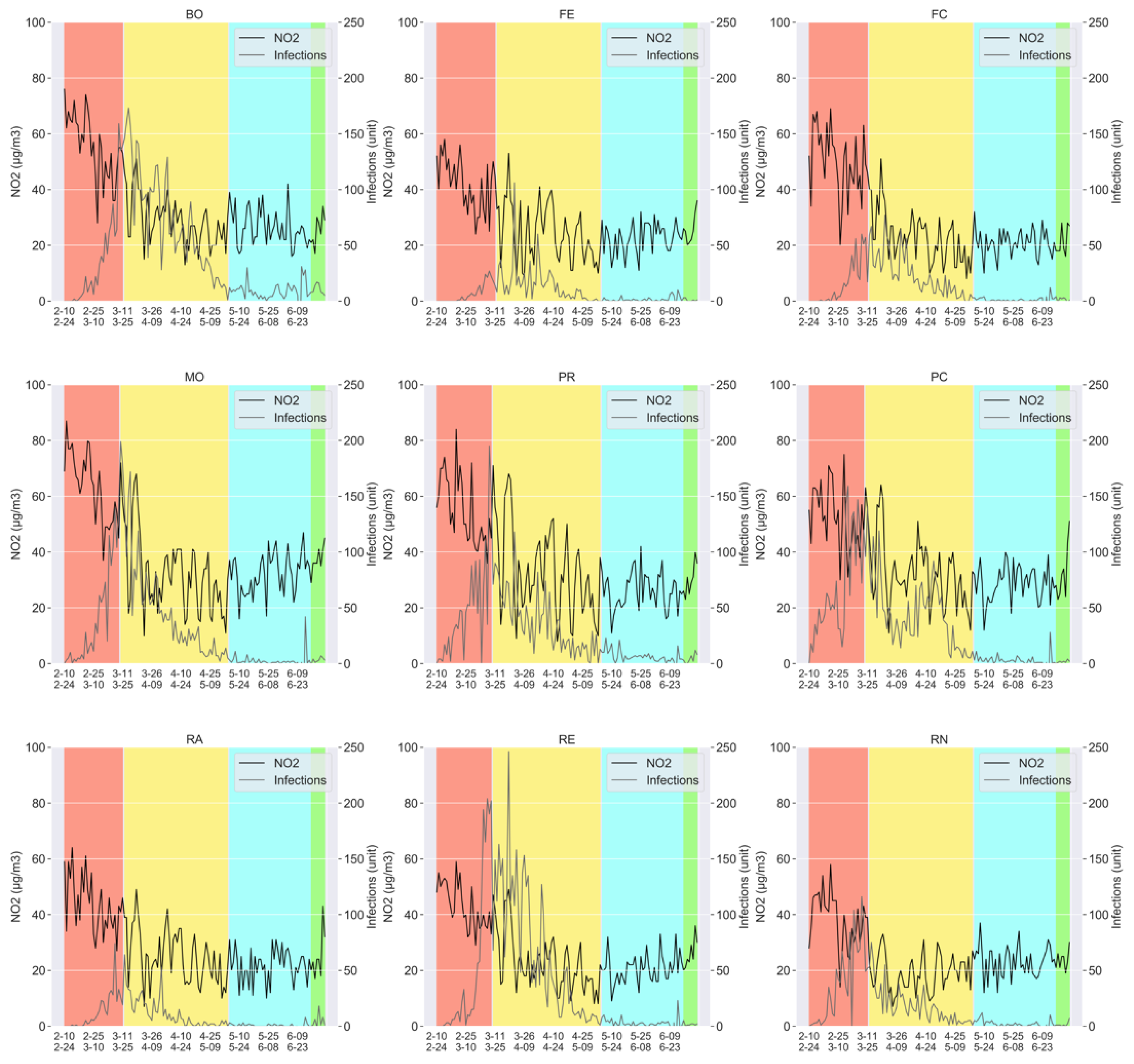
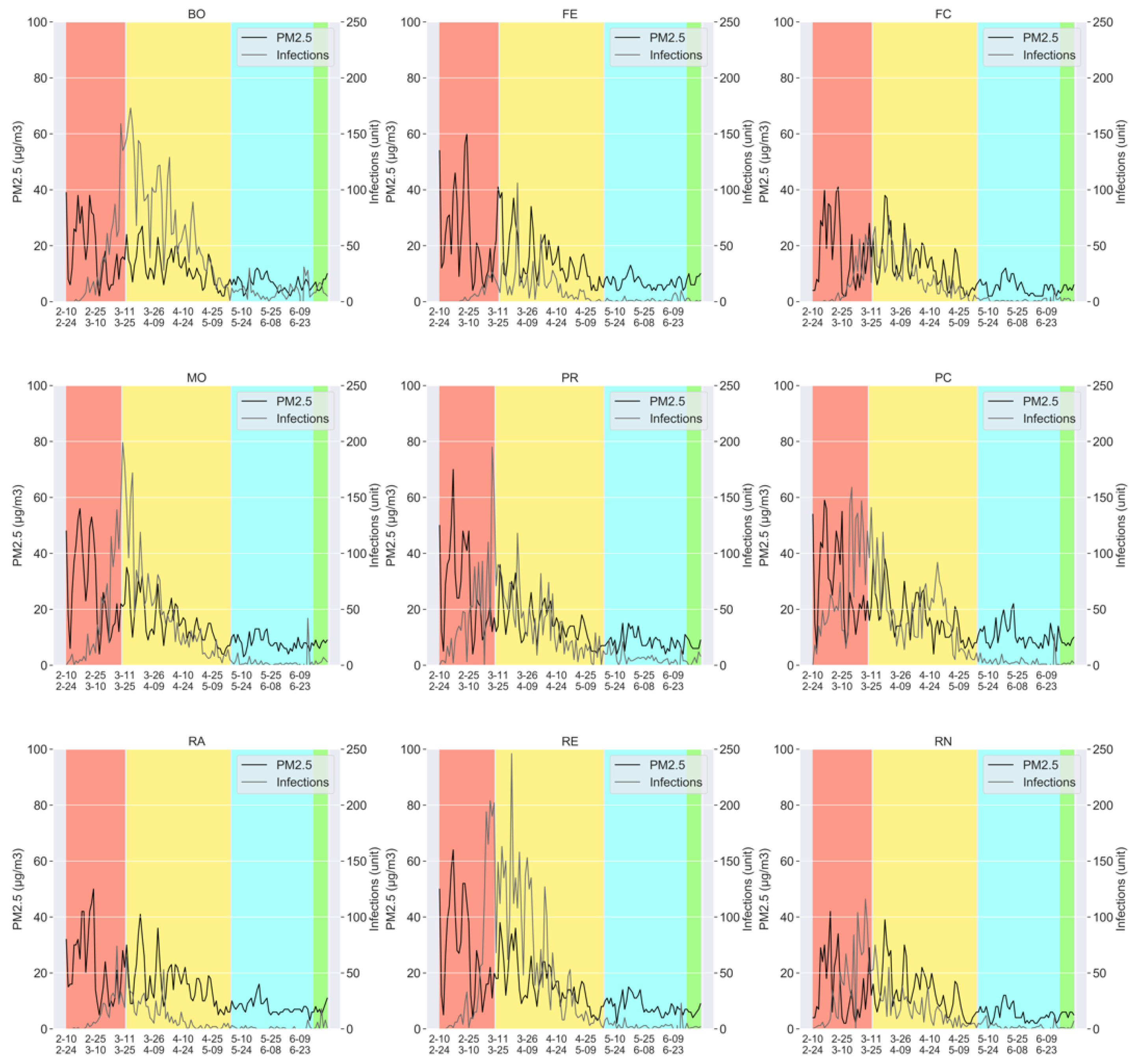
2.1. Preliminary Assumptions
- Phase 0: Prior to 8 March 2020, no specific restriction was imposed, which was valid for all the nine provinces of Emilia-Romagna, except for some local control measures (for example, for schools and universities);
- Phase 2: On 4 May 2020, the lockdown was partially released, though with several commercial and industrial activities still suspended, as well as the obligation for people to stay in quarantine if found or suspected ill, wear cloth face covering in public settings, wash hands frequently, etc., and where a social distancing of at least 1 meter and a half was difficult to maintain [34];
- Phase 3: On 14 June 2020, the lockdown was almost completely removed, with almost all activities resuming, provided that the personal protection measures mentioned above were obeyed [19].
2.2. Dataset Description
- The measurements of the particulate pollutants: PM2.5, PM10, and N02; taken on a daily basis, for all the aforementioned provinces (Bologna, Ferrara, Forlì-Cesena, Modena, Parma, Piacenza, Reggio nell’Emilia, Rimini, and Ravenna).
- The number of the daily COVID-19 infections, again for all the provinces mentioned above.
2.3. What Kind of Predictions Are We Looking for?
- (i)
- The former, with all those days with a number y of daily infections, equal or smaller than 17; and
- (ii)
- The latter, with those days registering a number of new infected people larger than 17.
2.4. Model Selection
3. Results: Predictions
3.1. Predictions: 2019->2020
- Bologna (0);
- Ferrara (1);
- Forlì-Cesena (2);
- Modena (1);
- Parma (16);
- Piacenza (23);
- Ravenna (0);
- Reggio Emilia (1);
- Rimini (1).
3.2. Predictions: 2017–2019->2020
- Bologna (1);
- Ferrara (0);
- Forlì-Cesena (0);
- Modena (0);
- Parma (29);
- Piacenza (43);
- Ravenna (0);
- Reggio Emilia (1);
- Rimini (0).
3.3. Predictions: What Happens If Personal Protection Measures Are Not Respected?
4. Discussion and Conclusions
Author Contributions
Funding
Conflicts of Interest
References
- Jamieson, A. Coronavirus Crisis May Get Worse and Worse and Worse, Warns WHO. Available online: https://www.independent.co.uk/news/uk/home-news/coronavirus-cases-deaths-who-infection-rate-global-latest-a9616366.html?fbclid=IwAR1rTs52bD1jZBjNEYNt63OuN_DweUkCHlB5oQAAExD2JAR-TXpc5pL2-QA (accessed on 18 July 2020).
- World Health Organization (WHO). Coronavirus Disease (COVID-2019) Situation Reports. Available online: https://www.who.int/emergencies/diseases/novel-coronavirus-2019/situation-reports (accessed on 18 July 2020).
- Dipartimento Della Protezione Civile, Italia. Aggiornamento Casi COVID-19. Available online: http://opendatadpc.maps.arcgis.com/apps/opsdashboard/index.html#/b0c68bce2cce478eaac82fe38d4138b1 (accessed on 18 July 2020).
- Mehta, D. Moody’s: Italy’s GDP to Contract 9.3% in 2020. FXStreet. 2020. Available online: https://www.fxstreet.com/news/moodys-italys-gdp-to-contract-93-in-2020-202004300541 (accessed on 18 July 2020).
- Carey, B. Can an Algorithm Predict the Pandemic’s Next Moves? The New York Times. 2020. Available online: https://www.nytimes.com/2020/07/02/health/santillana-coronavirus-model-forecast.html?smid=fb-share&fbclid=IwAR15B7tGHRL8oyL1NHgjXyGojTSYbHpoO0ww8hG85B2bN7NVMxJVK2da5wU (accessed on 18 July 2020).
- Delnevo, G.; Mirri, S.; Roccetti, M. Particulate Matter and COVID-19 disease diffusion in Emilia-Romagna (Italy). Already a cold case? Computation 2020, 8, 59. [Google Scholar] [CrossRef]
- Granger, C. Investigating causal relations by econometric models and cross-spectral methods. Econometrica 1969, 37, 424–438. [Google Scholar] [CrossRef]
- Maziarz, M. A review of the Granger-causality fallacy. J. Philos. Econ. 2015, 8, 86–105. [Google Scholar]
- Conticini, E.; Frediani, B.; Caro, D. Can atmospheric pollution be considered a co-factor in extremely high level of SARS-CoV-2 lethality in Northern Italy? Environ. Pollut. 2020, 261, 114465. [Google Scholar] [CrossRef] [PubMed]
- Becchetti, L.; Conzo, G.; Conzo, P.; Salustri, F. Understanding the Heterogeneity of Adverse COVID-19 Outcomes: The Role of Poor Quality of Air and Lockdown Decisions. Available online: https://papers.ssrn.com/sol3/papers.cfm?abstract_id=3572548 (accessed on 18 July 2020).
- Li, Q.; Guan, X.; Wu, P.; Wang, X.; Zhou, L.; Tong, Y.; Ren, R.; Leung, K.S.M.; Lau, E.H.Y.; Wong, J.Y.; et al. Early transmission dynamics in Wuhan, China, of novel coronavirus–infected pneumonia. N. Engl. J. Med. 2020, 382, 1199–1207. [Google Scholar] [CrossRef] [PubMed]
- Zhou, P.; Yang, X.L.; Wang, X.G.; Hu, B.; Zhang, L.; Zhang, W.; Si, H.R.; Zhu, Y.; Li, B.; Huang, C.L.; et al. A pneumonia outbreak associated with a new coronavirus of probable bat origin. Nature 2020, 579, 270–273. [Google Scholar] [CrossRef] [Green Version]
- Nunez Soza, L.; Jordanova, P.; Nicolis, L.; Strelec, L.; Stehlik, M. Small sample robust approach to outliers and correlation of Atmospheric Pollution and Health Effects in Santiago de Chile. Chemom. Intell. Lab. Syst. 2019, 185, 73–84. [Google Scholar] [CrossRef]
- Morawska, L.; Milton, D.K. It is time to address airborne transmission of COVID-19. Clin. Infect. Dis. 2020. [Google Scholar] [CrossRef]
- Setti, L.; Passarini, F.; De Gennaro, G.; Barbieri, P.; Perrone, M.G.; Borelli, M.; Palmisani, J.; Di Gilio, A.; Priscitelli, P.; Miani, A. SARS-Cov-2RNA found on particulate matter of Bergamo in Northern Italy: T First evidence. Environ. Res. 2020, 188, 109754. [Google Scholar] [CrossRef]
- Ferrarotti, M.J.; Cavalli, A. On the Hypothesis of Particulate Matter as Carrier of SARS-CoV-2. Numerical Findings with a Novel Package for Smoluchowski Aggregation Via Direct Monte Carlo; Preprint, n 1; Department of Chemistry, University of Bologna: Bologna, Italy, 2020. [Google Scholar]
- Setti, L.; Passarini, F.; De Gennaro, G.; Barbieri, P.; Perrone, M.G.; Borelli, M.; Palmisani, J.; Di Gilio, A.; Priscitelli, P.; Miani, A. Airborne Transmission Route of COVID-19: Why 2 Meters/6 Feet of Inter-Personal Distance Could Not Be Enough. Int. J. Environ. Res. Public Health 2020, 17, 2932. [Google Scholar] [CrossRef] [Green Version]
- Setti, L.; Passarini, F.; De Gennaro, G.; Barbieri, P.; Perrone, M.G.; Borelli, M.; Palmisani, J.; Di Gilio, A.; Priscitelli, P.; Miani, A. Searching for SARS-COV-2 on Particulate Matter: A Possible Early Indicator of COVID-19 Epidemic Recurrence. Int. J. Environ. Res. Public Health 2020, 17, 2986. [Google Scholar] [CrossRef] [PubMed]
- Gazzetta Ufficiale della Repubblica Italiana. Decreto del Presidente del Consiglio dei Ministri 11 Giugno 2020. Available online: https://www.gazzettaufficiale.it/eli/id/2020/06/11/20A03194/sg (accessed on 19 July 2020).
- Kogan, N.E.; Clemente, L.; Liautaud, P.; Kaashoek, J.; Link, N.B.; Nguyen, A.T.; Lu, F.S.; Huybers, P.; Resch, B.; Havas, C.; et al. An early warning approach to monitor COVID-19 activity with multiple digital traces in near real-time. arXiv 2020, arXiv:2007.00756. [Google Scholar]
- Fox, G.N.; Moawad, N.S. UpToDate: A comprehensive clinical database. J. Family Pract. 2003, 52, 706–710. [Google Scholar]
- Buchanan, M. The limits of machine prediction. Nat. Phys. 2019, 15, 304. [Google Scholar] [CrossRef]
- Kermack, W.O.; McKendrick, A.G. Contributions to the mathematical theory of epidemics—I. Bull. Math. Boil. 1991, 53, 33–55. [Google Scholar]
- Russell, S.J.; Norvig, P. Artificial Intelligence: A Modern Approach. Prentice Hall 2010. Available online: https://www.google.com.hk/url?sa=t&rct=j&q=&esrc=s&source=web&cd=&ved=2ahUKEwi2m73KubPrAhVPPnAKHeURBS8QFjACegQIBhAB&url=https%3A%2F%2Ffaculty.psau.edu.sa%2Ffiledownload%2Fdoc-7-pdf-a154ffbcec538a4161a406abf62f5b76-original.pdf&usg=AOvVaw0i7pLrlBs9LMW296xeV6b0 (accessed on 18 July 2020).
- Ardabili, S.F.; Mosavi, A.; Ghamisi, P.; Ferdinand, F.; Varkonyi-Koczy, A.R.; Reuter, U.; Rabczuck, T.; Atkinson, P.M. COVID-19 outbreak prediction with machine learning. medRxiv Prepr. 2020. Available online: https://www.medrxiv.org/content/10.1101/2020.04.17.20070094v1.full.pdf (accessed on 18 July 2020).
- Tuli, S.; Tuli, S.; Tuli, R.; Gill, S.S. Predicting the Growth and Trend of COVID-19 Pandemic using Machine Learning and Cloud Computing. Internet Things 2020, 2020, 100222. [Google Scholar] [CrossRef]
- Liu, Y.; Wang, Z.; Ren, J.; Tian, Y.; Zhou, M.; Zhou, T.; Ye, K.; Zhao, Y.; Qiu, Y.; Li, J. A COVID-19 Risk Assessment Decision Support System for General Practitioners: Design and Development Study. J. Med. Internet Res. 2020, 22, e19786. [Google Scholar] [CrossRef]
- Nguyen, T.T. Artificial Intelligence in the Battle Against Coronavirus (COVID-19): A Survey and Future Research Directions. Preprint 2020. Available online: https://figshare.com/articles/Artificial_Intelligence_in_the_Battle_against_Coronavirus_COVID-19_A_Survey_and_Future_Research_Directions/12127020 (accessed on 18 July 2020).
- Alimadadi, A.; Aryal, S.; Manandhar, I.; Munroe, P.B.; Joe, B.; Cheng, X. Artificial intelligence and machine learning to fight COVID-19. Physiol. Genomics 2020, 52, 200–202. [Google Scholar] [CrossRef]
- Naudé, W. Artificial Intelligence against COVID-19: An Early Review. Available online: https://www.iza.org/publications/dp/13110/artificial-intelligence-against-covid-19-an-early-review (accessed on 18 July 2020).
- Kucharski, A.J.; Russell, T.W.; Diamond, C.; Liu, Y.; Edmunds, J.; Funk, S.; Eggo, R.M. Early dynamics of transmission and control of COVID-19: A mathematical modelling study. Lancet Infect. Dis. 2020, 20, 553–558. [Google Scholar] [CrossRef] [Green Version]
- Gazzetta Ufficiale della Repubblica Italiana. Decreto del Presidente del Consiglio dei Ministri 8 Marzo 2020. Available online: https://www.gazzettaufficiale.it/eli/id/2020/03/08/20A01522/sg (accessed on 18 July 2020).
- Governo Italiano Presidenza del Consiglio dei Ministri. Available online: http://www.governo.it/it/articolo/firmato-il-dpcm-9-marzo-2020/14276 (accessed on 18 July 2020).
- Gazzetta Ufficiale della Repubblica Italiana. Decreto del Presidente del Consiglio dei Ministri 26 Aprile 2020. Available online: https://www.gazzettaufficiale.it/eli/id/2020/04/27/20A02352/sg (accessed on 18 July 2020).
- COVID-19 Italia—Monitoraggio Situazione. Available online: https://github.com/pcm-dpc/COVID-19 (accessed on 18 July 2020).
- Arpae Emilia-Romagna. Available online: https://arpae.it/mappa_qa.asp?idlivello=1682&tema=stazioni (accessed on 18 July 2020).
- Lauer, S.A.; Grantz, K.H.; Bi, Q.; Jones, F.K.; Zheng, Q.; Meredith, H.R.; Azman, A.S.; Reich, N.G.; Lessler, J. The incubation period of coronavirus disease 2019 (COVID-19) from publicly reported confirmed cases: Estimation and application. Ann. Intern. Med. 2020, 172, 577–582. [Google Scholar] [CrossRef] [Green Version]
- K Keller, J.M.; Gray, M.R.; Givens, J.A. A fuzzy k-nearest neighbor algorithm. IEEE Trans. Syst. Man Cybern. 1985, 4, 580–585. [Google Scholar] [CrossRef]
- Lawrence, R.L.; Wright, A. Rule-based classification systems using classification and regression tree (CART) analysis. Photogramm. Eng. Remote Sens. 2001, 67, 1137–1142. [Google Scholar]
- Cortes, C.; Vapnik, V. Support-vector networks. Mach. Learn. 1995, 20, 273–297. [Google Scholar] [CrossRef]
- Hastie, T.; Tibshirani, R.; Friedman, J.; Franklin, J. The elements of statistical learning: Data mining, inference and prediction. Math. Intell. 2005, 27, 83–85. [Google Scholar]
- Dietterich, T.G. Ensemble methods in machine learning. In Proceedings of the First International Workshop on Multiple Classifier Systems, Cagliari, Italy, 21–23 June 2000; Springer: Berlin, Germany, 2000; pp. 1–15. [Google Scholar]
- Friedman, J.H. Stochastic gradient boosting. Comput. Stat. Data Anal. 2002, 38, 367–378. [Google Scholar] [CrossRef]
- Barandiaran, I. The random subspace method for constructing decision forests. IEEE Trans. Pattern Anal. Mach. Intell. 1998, 20, 1–22. [Google Scholar]
- Geurts, P.; Ernst, D.; Wehenkel, L. Extremely randomized trees. Mach. Learn. 2006, 63, 3–42. [Google Scholar] [CrossRef] [Green Version]
- Cohen, A.J.; Brauer, M.; Burnett, R.; Ross Anderson, H.; Frostad, J.; Estep, K.; Balakrishnan, K.; Brunekreef, B.; Dandona, L.; Dandona, R.; et al. Estimates and 25-year trends of the global burden of disease attributable to ambient air pollution: an analysis of data from the Global Burden of Diseases. Lancet 2017, 389, 215. [Google Scholar] [CrossRef] [Green Version]
- Carbone, M.; Green, J.B.; Bucci, E.M.; Lednicky, J.A. Coronaviruses: Facts, Myths, and Hypotheses. J. Thorac. Oncol. 2020, 15, 675–678. [Google Scholar] [CrossRef]
- Delnevo, G.; Roccetti, M.; Mirri, S. Modeling Patients’ Online Medical Conversations: A Granger Causality Approach. In Proceedings of the 2018 IEEE/ACM International Conference on Connected Health: Applications, Systems and Engineering Technologies, Washington, DC, USA, 26–28 September 2018; IEEE: Piscataway, NJ, USA, 2018; pp. 40–44. [Google Scholar]


| Pollution | Lag | KNN | CART | SVC | MLP | AB | GB | RF | ET |
|---|---|---|---|---|---|---|---|---|---|
| All | 1 | 0.81 ± 0.03 | 0.75 ± 0.05 | 0.81 ± 0.04 | 0.84 ± 0.03 | 0.78 ± 0.05 | 0.81 ± 0.04 | 0.81 ± 0.03 | 0.78 ± 0.04 |
| 2 | 0.81 ± 0.03 | 0.81 ± 0.04 | 0.83 ± 0.03 | 0.84 ± 0.04 | 0.79 ± 0.05 | 0.83 ± 0.03 | 0.84 ± 0.05 | 0.83 ± 0.04 | |
| 3 | 0.83 ± 0.05 | 0.78 ± 0.05 | 0.83 ± 0.04 | 0.84 ± 0.04 | 0.81 ± 0.04 | 0.83 ± 0.02 | 0.85 ± 0.03 | 0.85 ± 0.03 | |
| 4 | 0.82 ± 0.04 | 0.78 ± 0.05 | 0.84 ± 0.04 | 0.84 ± 0.05 | 0.81 ± 0.03 | 0.84 ± 0.03 | 0.84 ± 0.03 | 0.85 ± 0.03 | |
| 5 | 0.85 ± 0.03 | 0.82 ± 0.05 | 0.85 ± 0.03 | 0.86 ± 0.04 | 0.82 ± 0.05 | 0.86 ± 0.04 | 0.87 ± 0.04 | 0.86 ± 0.03 | |
| 6 | 0.86 ± 0.03 | 0.82 ± 0.05 | 0.87 ± 0.03 | 0.86 ± 0.03 | 0.82 ± 0.04 | 0.86 ± 0.03 | 0.85 ± 0.04 | 0.88 ± 0.03 | |
| 7 | 0.86 ± 0.03 | 0.83 ± 0.04 | 0.87 ± 0.03 | 0.87 ± 0.02 | 0.84 ± 0.03 | 0.85 ± 0.03 | 0.86 ± 0.03 | 0.87 ± 0.04 | |
| 8 | 0.87 ± 0.02 | 0.84 ± 0.04 | 0.89 ± 0.03 | 0.89 ± 0.02 | 0.82 ± 0.03 | 0.86 ± 0.03 | 0.86 ± 0.04 | 0.90 ± 0.03 | |
| PM2.5 | 1 | 0.79 ± 0.03 | 0.77 ± 0.04 | 0.80 ± 0.04 | 0.81 ± 0.03 | 0.78 ± 0.06 | 0.81 ± 0.03 | 0.76 ± 0.03 | 0.77 ± 0.04 |
| 2 | 0.80 ± 0.04 | 0.78 ± 0.05 | 0.82 ± 0.04 | 0.82 ± 0.04 | 0.78 ± 0.04 | 0.82 ± 0.04 | 0.81 ± 0.03 | 0.79 ± 0.03 | |
| 3 | 0.81 ± 0.03 | 0.79 ± 0.05 | 0.82 ± 0.03 | 0.82 ± 0.04 | 0.81 ± 0.03 | 0.84 ± 0.03 | 0.83 ± 0.03 | 0.82 ± 0.03 | |
| 4 | 0.80 ± 0.03 | 0.81 ± 0.04 | 0.85 ± 0.02 | 0.83 ± 0.03 | 0.81 ± 0.03 | 0.85 ± 0.04 | 0.85 ± 0.03 | 0.83 ± 0.03 | |
| 5 | 0.84 ± 0.03 | 0.82 ± 0.04 | 0.86 ± 0.03 | 0.85 ± 0.04 | 0.81 ± 0.04 | 0.86 ± 0.04 | 0.87 ± 0.03 | 0.85 ± 0.02 | |
| 6 | 0.85 ± 0.04 | 0.84 ± 0.04 | 0.87 ± 0.03 | 0.87 ± 0.03 | 0.82 ± 0.04 | 0.87 ± 0.04 | 0.87 ± 0.03 | 0.87 ± 0.03 | |
| 7 | 0.85 ± 0.04 | 0.85 ± 0.03 | 0.87 ± 0.03 | 0.86 ± 0.02 | 0.82 ± 0.05 | 0.86 ± 0.04 | 0.88 ± 0.03 | 0.88 ± 0.03 | |
| 8 | 0.88 ± 0.03 | 0.84 ± 0.04 | 0.88 ± 0.03 | 0.87 ± 0.03 | 0.83 ± 0.05 | 0.86 ± 0.03 | 0.87 ± 0.04 | 0.89 ± 0.04 | |
| PM10 | 1 | 0.79 ± 0.05 | 0.77 ± 0.03 | 0.80 ± 0.04 | 0.81 ± 0.04 | 0.78 ± 0.05 | 0.81 ± 0.04 | 0.78 ± 0.05 | 0.79 ± 0.04 |
| 2 | 0.81 ± 0.04 | 0.79 ± 0.05 | 0.81 ± 0.04 | 0.82 ± 0.04 | 0.78 ± 0.04 | 0.82 ± 0.03 | 0.82 ± 0.05 | 0.82 ± 0.04 | |
| 3 | 0.80 ± 0.03 | 0.77 ± 0.03 | 0.82 ± 0.03 | 0.83 ± 0.04 | 0.80 ± 0.03 | 0.83 ± 0.03 | 0.83 ± 0.04 | 0.83 ± 0.03 | |
| 4 | 0.83 ± 0.03 | 0.78 ± 0.03 | 0.84 ± 0.03 | 0.84 ± 0.04 | 0.80 ± 0.02 | 0.85 ± 0.04 | 0.84 ± 0.02 | 0.84 ± 0.03 | |
| 5 | 0.84 ± 0.04 | 0.81 ± 0.06 | 0.85 ± 0.03 | 0.86 ± 0.03 | 0.80 ± 0.05 | 0.87 ± 0.04 | 0.86 ± 0.03 | 0.85 ± 0.03 | |
| 6 | 0.85 ± 0.03 | 0.82 ± 0.04 | 0.86 ± 0.03 | 0.87 ± 0.03 | 0.82 ± 0.04 | 0.86 ± 0.04 | 0.86 ± 0.04 | 0.85 ± 0.04 | |
| 7 | 0.87 ± 0.03 | 0.85 ± 0.04 | 0.88 ± 0.03 | 0.87 ± 0.03 | 0.83 ± 0.05 | 0.87 ± 0.04 | 0.87 ± 0.03 | 0.88 ± 0.03 | |
| 8 | 0.87 ± 0.02 | 0.85 ± 0.03 | 0.88 ± 0.03 | 0.88 ± 0.03 | 0.82 ± 0.04 | 0.88 ± 0.04 | 0.87 ± 0.04 | 0.89 ± 0.03 | |
| NO2 | 1 | 0.80 ± 0.04 | 0.78 ± 0.03 | 0.81 ± 0.03 | 0.81 ± 0.04 | 0.78 ± 0.04 | 0.80 ± 0.04 | 0.77 ± 0.03 | 0.78 ± 0.03 |
| 2 | 0.79 ± 0.03 | 0.76 ± 0.04 | 0.81 ± 0.02 | 0.82 ± 0.02 | 0.79 ± 0.05 | 0.81 ± 0.03 | 0.80 ± 0.04 | 0.79 ± 0.04 | |
| 3 | 0.82 ± 0.03 | 0.77 ± 0.03 | 0.82 ± 0.03 | 0.83 ± 0.03 | 0.80 ± 0.03 | 0.82 ± 0.04 | 0.83 ± 0.02 | 0.83 ± 0.02 | |
| 4 | 0.85 ± 0.02 | 0.80 ± 0.02 | 0.83 ± 0.03 | 0.84 ± 0.04 | 0.80 ± 0.04 | 0.83 ± 0.03 | 0.86 ± 0.03 | 0.85 ± 0.02 | |
| 5 | 0.86 ± 0.02 | 0.81 ± 0.03 | 0.84 ± 0.03 | 0.85 ± 0.04 | 0.82 ± 0.04 | 0.83 ± 0.03 | 0.87 ± 0.03 | 0.85 ± 0.02 | |
| 6 | 0.86 ± 0.03 | 0.83 ± 0.04 | 0.85 ± 0.03 | 0.86 ± 0.04 | 0.80 ± 0.04 | 0.84 ± 0.04 | 0.87 ± 0.03 | 0.86 ± 0.03 | |
| 7 | 0.85 ± 0.03 | 0.82 ± 0.05 | 0.85 ± 0.02 | 0.85 ± 0.03 | 0.81 ± 0.04 | 0.84 ± 0.04 | 0.87 ± 0.04 | 0.87 ± 0.03 | |
| 8 | 0.86 ± 0.03 | 0.81 ± 0.03 | 0.86 ± 0.02 | 0.86 ± 0.03 | 0.81 ± 0.04 | 0.85 ± 0.04 | 0.87 ± 0.03 | 0.88 ± 0.02 |
| Algorithm | Testing | |||
|---|---|---|---|---|
| Class | Precision | Recall | F1 Score | |
| KNN | <=17 | 0.90 | 0.85 | 0.845 |
| >17 | 0.75 | 0.82 | ||
| SVC | <=17 | 0.95 | 0.87 | 0.890 |
| >17 | 0.80 | 0.92 | ||
| MLP | <=17 | 0.93 | 0.90 | 0.890 |
| >17 | 0.82 | 0.87 | ||
| GB | <=17 | 0.92 | 0,91 | 0.893 |
| >17 | 0.84 | 0.86 | ||
| RF | <=17 | 0.93 | 0.87 | 0.878 |
| >17 | 0.79 | 0.88 | ||
| ET | <=17 | 0.91 | 0.91 | 0.881 |
| >17 | 0.83 | 0.84 | ||
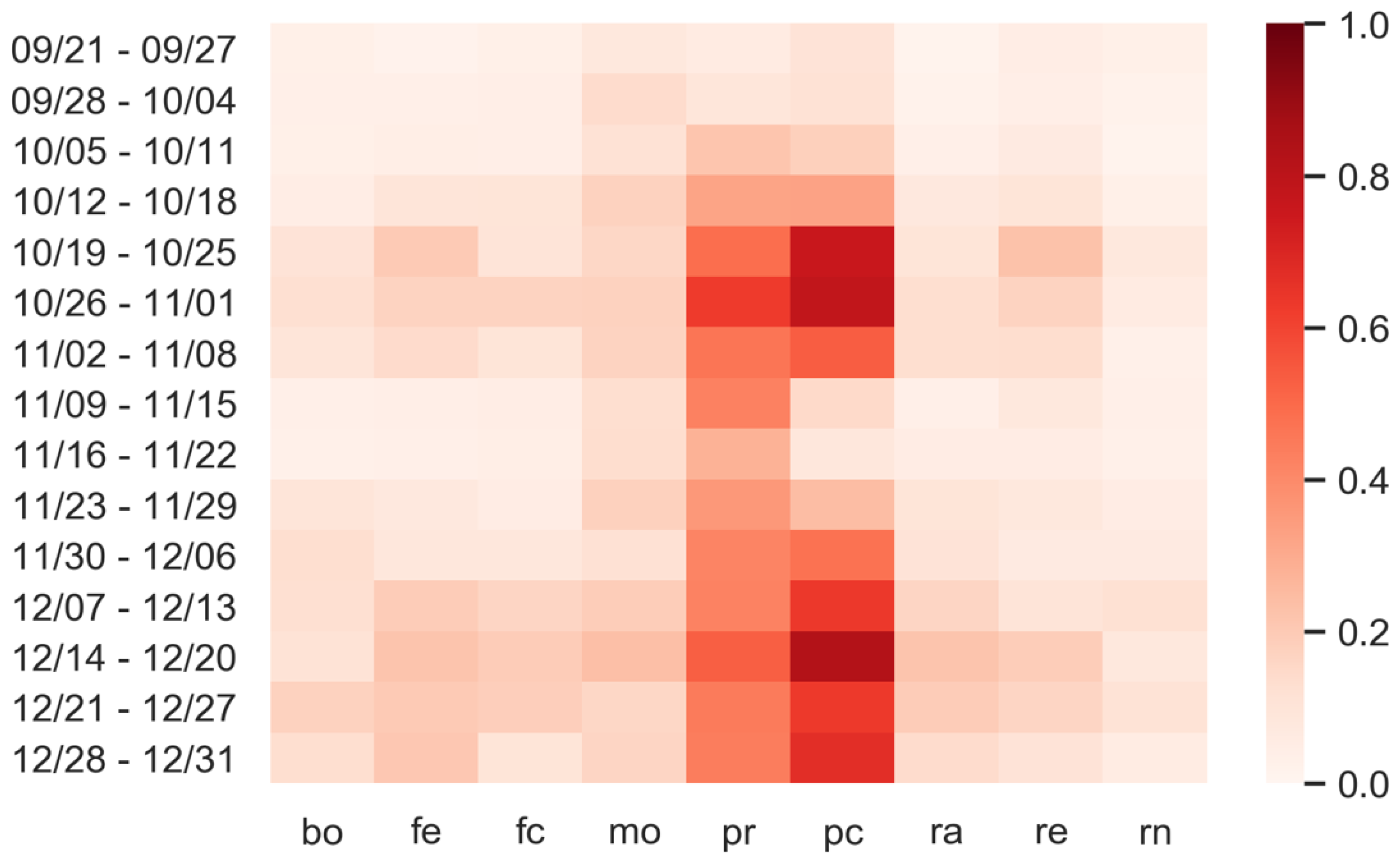
| Day | Bo | Fe | Fc | Mo | Pr | Pc | Ra | Re | Rn |
|---|---|---|---|---|---|---|---|---|---|
| 9/21 | 0.00 | 0.00 | 0.00 | 0.02 | 0.01 | 0.35 | 0.00 | 0.01 | 0.00 |
| 9/22 | 0.04 | 0.00 | 0.04 | 0.11 | 0.11 | 0.38 | 0.03 | 0.03 | 0.00 |
| 9/23 | 0.1 | 0.08 | 0.07 | 0.18 | 0.3 | 0.15 | 0.08 | 0.22 | 0.07 |
| 9/24 | 0.14 | 0.17 | 0.17 | 0.27 | 0.11 | 0.31 | 0.14 | 0.12 | 0.11 |
| 9/25 | 0.01 | 0.01 | 0.01 | 0.19 | 0.24 | 0.09 | 0.00 | 0.07 | 0.01 |
| 9/26 | 0.00 | 0.01 | 0.01 | 0.01 | 0.11 | 0.12 | 0.00 | 0.03 | 0.00 |
| 9/27 | 0.00 | 0.01 | 0.00 | 0.1 | 0.06 | 0.07 | 0.03 | 0.02 | 0.01 |
| 9/28 | 0.00 | 0.02 | 0.01 | 0.05 | 0.2 | 0.09 | 0.02 | 0.06 | 0.01 |
| 9/29 | 0.14 | 0.00 | 0.04 | 0.23 | 0.04 | 0.02 | 0.16 | 0.04 | 0.02 |
| 9/30 | 0.03 | 0.01 | 0.01 | 0.04 | 0.01 | 0.02 | 0.06 | 0.01 | 0.02 |
| 10/1 | 0.01 | 0.01 | 0.01 | 0.02 | 0.01 | 0.04 | 0.01 | 0.02 | 0.00 |
| 10/2 | 0.00 | 0.01 | 0.05 | 0.23 | 0.53 | 0.07 | 0.00 | 0.12 | 0.00 |
| 10/3 | 0.00 | 0.02 | 0.03 | 0.13 | 0.54 | 0.46 | 0.02 | 0.25 | 0.01 |
| 10/4 | 0.04 | 0.04 | 0.01 | 0.17 | 0.16 | 0.19 | 0.00 | 0.05 | 0.09 |
| 10/5 | 0.01 | 0.03 | 0.00 | 0.03 | 0.02 | 0.15 | 0.02 | 0.00 | 0.00 |
| 10/6 | 0.01 | 0.02 | 0.00 | 0.02 | 0.16 | 0.19 | 0.00 | 0.03 | 0.00 |
| 10/7 | 0.01 | 0.00 | 0.1 | 0.25 | 0.59 | 0.73 | 0.00 | 0.03 | 0.00 |
| 10/8 | 0.01 | 0.00 | 0.00 | 0.12 | 0.09 | 0.39 | 0.02 | 0.19 | 0.02 |
| 10/9 | 0.00 | 0.00 | 0.01 | 0.02 | 0.21 | 0.15 | 0.03 | 0.00 | 0.01 |
| 10/10 | 0.00 | 0.00 | 0.00 | 0.01 | 0.01 | 0.07 | 0.00 | 0.00 | 0.00 |
| 10/11 | 0.07 | 0.01 | 0.00 | 0.01 | 0.01 | 0.04 | 0.00 | 0.00 | 0.00 |
| 10/12 | 0.03 | 0.18 | 0.02 | 0.21 | 0.04 | 0.42 | 0.02 | 0.01 | 0.00 |
| 10/13 | 0.01 | 0.01 | 0.01 | 0.06 | 0.08 | 0.37 | 0.01 | 0.04 | 0.00 |
| 10/14 | 0.00 | 0.00 | 0.01 | 0.01 | 0.03 | 0.02 | 0.00 | 0.00 | 0.00 |
| 10/15 | 0.01 | 0.01 | 0.01 | 0.05 | 0.16 | 0.02 | 0.00 | 0.01 | 0.00 |
| 10/16 | 0.08 | 0.04 | 0.4 | 0.35 | 0.29 | 0.1 | 0.1 | 0.15 | 0.00 |
| 10/17 | 0.11 | 0.37 | 0.09 | 0.39 | 0.47 | 0.45 | 0.25 | 0.18 | 0.08 |
| 10/18 | 0.06 | 0.01 | 0.05 | 0.04 | 0.02 | 0.02 | 0.02 | 0.04 | 0.06 |
| 10/19 | 0.01 | 0.04 | 0.01 | 0.16 | 0.45 | 0.14 | 0.2 | 0.09 | 0.02 |
| 10/20 | 0.04 | 0.4 | 0.04 | 0.2 | 0.74 | 0.81 | 0.06 | 0.38 | 0.07 |
| 10/21 | 0.07 | 0.03 | 0.06 | 0.07 | 0.4 | 0.64 | 0.09 | 0.07 | 0.09 |
| 10/22 | 0.01 | 0.02 | 0.01 | 0.08 | 0.45 | 0.51 | 0.02 | 0.1 | 0.01 |
| 10/23 | 0.03 | 0.07 | 0.01 | 0.14 | 0.44 | 0.46 | 0.02 | 0.04 | 0.02 |
| 10/24 | 0.04 | 0.06 | 0.09 | 0.17 | 0.56 | 0.49 | 0.02 | 0.03 | 0.02 |
| 10/25 | 0.03 | 0.02 | 0.02 | 0.22 | 0.14 | 0.35 | 0.01 | 0.04 | 0.01 |
| 10/26 | 0.03 | 0.04 | 0.09 | 0.17 | 0.26 | 0.64 | 0.04 | 0.1 | 0.00 |
| 10/27 | 0.01 | 0.01 | 0.00 | 0.01 | 0.06 | 0.07 | 0.01 | 0.00 | 0.00 |
| 10/28 | 0.01 | 0.02 | 0.04 | 0.19 | 0.53 | 0.13 | 0.01 | 0.04 | 0.01 |
| 10/29 | 0.03 | 0.59 | 0.68 | 0.33 | 0.79 | 0.74 | 0.28 | 0.35 | 0.18 |
| 10/30 | 0.03 | 0.07 | 0.04 | 0.04 | 0.19 | 0.09 | 0.02 | 0.03 | 0.05 |
| 10/31 | 0.02 | 0.01 | 0.02 | 0.02 | 0.42 | 0.44 | 0.02 | 0.11 | 0.03 |
| 11/1 | 0.12 | 0.34 | 0.12 | 0.09 | 0.22 | 0.13 | 0.45 | 0.03 | 0.05 |
| 11/2 | 0.06 | 0.33 | 0.05 | 0.4 | 0.82 | 0.71 | 0.1 | 0.3 | 0.07 |
| 11/3 | 0.03 | 0.24 | 0.02 | 0.17 | 0.38 | 0.78 | 0.06 | 0.03 | 0.03 |
| 11/4 | 0.14 | 0.06 | 0.08 | 0.25 | 0.42 | 0.55 | 0.09 | 0.03 | 0.03 |
| 11/5 | 0.09 | 0.17 | 0.14 | 0.13 | 0.62 | 0.4 | 0.09 | 0.16 | 0.15 |
| 11/6 | 0.04 | 0.06 | 0.11 | 0.05 | 0.12 | 0.15 | 0.05 | 0.02 | 0.07 |
| 11/7 | 0.05 | 0.08 | 0.25 | 0.08 | 0.72 | 0.51 | 0.13 | 0.14 | 0.13 |
| 11/8 | 0.03 | 0.06 | 0.08 | 0.08 | 0.45 | 0.32 | 0.09 | 0.02 | 0.04 |
| 11/9 | 0.13 | 0.03 | 0.04 | 0.13 | 0.19 | 0.08 | 0.35 | 0.06 | 0.21 |
| 11/10 | 0.03 | 0.00 | 0.03 | 0.06 | 0.03 | 0.01 | 0.03 | 0.01 | 0.1 |
| 11/11 | 0.01 | 0.00 | 0.00 | 0.00 | 0.05 | 0.07 | 0.01 | 0.06 | 0.02 |
| 11/12 | 0.04 | 0.00 | 0.07 | 0.02 | 0.18 | 0.09 | 0.03 | 0.05 | 0.13 |
| 11/13 | 0.04 | 0.05 | 0.03 | 0.01 | 0.02 | 0.03 | 0.01 | 0.02 | 0.05 |
| 11/14 | 0.01 | 0.01 | 0.01 | 0.01 | 0.01 | 0.03 | 0.01 | 0.01 | 0.00 |
| 11/15 | 0.00 | 0.00 | 0.00 | 0.01 | 0.01 | 0.08 | 0.00 | 0.01 | 0.00 |
| 11/16 | 0.00 | 0.00 | 0.01 | 0.23 | 0.22 | 0.22 | 0.01 | 0.22 | 0.00 |
| 11/17 | 0.06 | 0.03 | 0.02 | 0.1 | 0.05 | 0.07 | 0.02 | 0.01 | 0.00 |
| 11/18 | 0.32 | 0.1 | 0.22 | 0.06 | 0.09 | 0.03 | 0.39 | 0.05 | 0.06 |
| 11/19 | 0.14 | 0.00 | 0.11 | 0.08 | 0.06 | 0.05 | 0.02 | 0.52 | 0.01 |
| 11/20 | 0.00 | 0.00 | 0.01 | 0.16 | 0.08 | 0.12 | 0.01 | 0.01 | 0.00 |
| 11/21 | 0.09 | 0.03 | 0.17 | 0.01 | 0.02 | 0.07 | 0.12 | 0.01 | 0.00 |
| 11/22 | 0.15 | 0.06 | 0.11 | 0.12 | 0.04 | 0.05 | 0.11 | 0.02 | 0.06 |
| 11/23 | 0.01 | 0.01 | 0.01 | 0.02 | 0.03 | 0.01 | 0.00 | 0.02 | 0.00 |
| 11/24 | 0.03 | 0.03 | 0.02 | 0.09 | 0.1 | 0.57 | 0.01 | 0.04 | 0.01 |
| 11/25 | 0.02 | 0.00 | 0.55 | 0.03 | 0.01 | 0.54 | 0.08 | 0.01 | 0.16 |
| 11/26 | 0.03 | 0.02 | 0.09 | 0.01 | 0.02 | 0.04 | 0.01 | 0.00 | 0.03 |
| 11/27 | 0.29 | 0.13 | 0.15 | 0.11 | 0.12 | 0.1 | 0.03 | 0.11 | 0.00 |
| 11/28 | 0.08 | 0.05 | 0.03 | 0.11 | 0.1 | 0.00 | 0.09 | 0.01 | 0.01 |
| 11/29 | 0.01 | 0.00 | 0.03 | 0.07 | 0.24 | 0.05 | 0.01 | 0.07 | 0.01 |
| 11/30 | 0.02 | 0.00 | 0.37 | 0.02 | 0.02 | 0.16 | 0.01 | 0.13 | 0.04 |
| 12/1 | 0.03 | 0.05 | 0.03 | 0.04 | 0.13 | 0.16 | 0.05 | 0.01 | 0.03 |
| 12/2 | 0.05 | 0.02 | 0.02 | 0.05 | 0.47 | 0.04 | 0.01 | 0.01 | 0.01 |
| 12/3 | 0.01 | 0.12 | 0.08 | 0.21 | 0.15 | 0.07 | 0.04 | 0.07 | 0.16 |
| 12/4 | 0.01 | 0.00 | 0.37 | 0.03 | 0.33 | 0.02 | 0.02 | 0.24 | 0.01 |
| 12/5 | 0.01 | 0.01 | 0.02 | 0.04 | 0.02 | 0.01 | 0.01 | 0.00 | 0.01 |
| 12/6 | 0.06 | 0.03 | 0.01 | 0.21 | 0.08 | 0.01 | 0.16 | 0.01 | 0.01 |
| 12/7 | 0.01 | 0.12 | 0.48 | 0.17 | 0.39 | 0.28 | 0.1 | 0.05 | 0.29 |
| 12/8 | 0.05 | 0.05 | 0.2 | 0.2 | 0.41 | 0.19 | 0.05 | 0.25 | 0.04 |
| 12/9 | 0.07 | 0.06 | 0.03 | 0.02 | 0.07 | 0.06 | 0.05 | 0.04 | 0.00 |
| 12/10 | 0.02 | 0.01 | 0.23 | 0.11 | 0.21 | 0.05 | 0.02 | 0.02 | 0.16 |
| 12/11 | 0.13 | 0.06 | 0.05 | 0.29 | 0.38 | 0.61 | 0.05 | 0.1 | 0.01 |
| 12/12 | 0.07 | 0.18 | 0.05 | 0.11 | 0.12 | 0.2 | 0.07 | 0.03 | 0.02 |
| 12/13 | 0.23 | 0.14 | 0.13 | 0.13 | 0.03 | 0.26 | 0.21 | 0.1 | 0.05 |
| 12/14 | 0.14 | 0.03 | 0.29 | 0.3 | 0.47 | 0.57 | 0.1 | 0.08 | 0.03 |
| 12/15 | 0.25 | 0.09 | 0.25 | 0.16 | 0.69 | 0.84 | 0.3 | 0.34 | 0.47 |
| 12/16 | 0.12 | 0.18 | 0.08 | 0.14 | 0.52 | 0.78 | 0.18 | 0.07 | 0.4 |
| 12/17 | 0.09 | 0.1 | 0.11 | 0.08 | 0.46 | 0.63 | 0.1 | 0.11 | 0.08 |
| 12/18 | 0.06 | 0.05 | 0.04 | 0.18 | 0.21 | 0.8 | 0.06 | 0.04 | 0.02 |
| 12/19 | 0.18 | 0.16 | 0.15 | 0.12 | 0.44 | 0.87 | 0.19 | 0.19 | 0.18 |
| 12/20 | 0.17 | 0.3 | 0.07 | 0.28 | 0.39 | 0.92 | 0.28 | 0.04 | 0.26 |
| 12/21 | 0.04 | 0.13 | 0.17 | 0.31 | 0.61 | 0.69 | 0.15 | 0.27 | 0.28 |
| 12/22 | 0.14 | 0.34 | 0.14 | 0.15 | 0.61 | 0.77 | 0.45 | 0.42 | 0.05 |
| 12/23 | 0.21 | 0.23 | 0.23 | 0.13 | 0.46 | 0.49 | 0.21 | 0.39 | 0.14 |
| 12/24 | 0.32 | 0.12 | 0.08 | 0.26 | 0.48 | 0.46 | 0.2 | 0.08 | 0.06 |
| 12/25 | 0.09 | 0.13 | 0.08 | 0.16 | 0.4 | 0.33 | 0.15 | 0.16 | 0.02 |
| 12/26 | 0.1 | 0.04 | 0.09 | 0.18 | 0.55 | 0.57 | 0.11 | 0.11 | 0.09 |
| 12/27 | 0.06 | 0.04 | 0.01 | 0.04 | 0.33 | 0.48 | 0.03 | 0.02 | 0.01 |
| 12/28 | 0.07 | 0.02 | 0.12 | 0.12 | 0.27 | 0.21 | 0.03 | 0.02 | 0.07 |
| 12/29 | 0.38 | 0.14 | 0.36 | 0.55 | 0.71 | 0.19 | 0.15 | 0.26 | 0.53 |
| 12/30 | 0.4 | 0.32 | 0.27 | 0.44 | 0.23 | 0.29 | 0.04 | 0.14 | 0.29 |
| 12/31 | 0.02 | 0.01 | 0.01 | 0.01 | 0.04 | 0.4 | 0.1 | 0.01 | 0.00 |
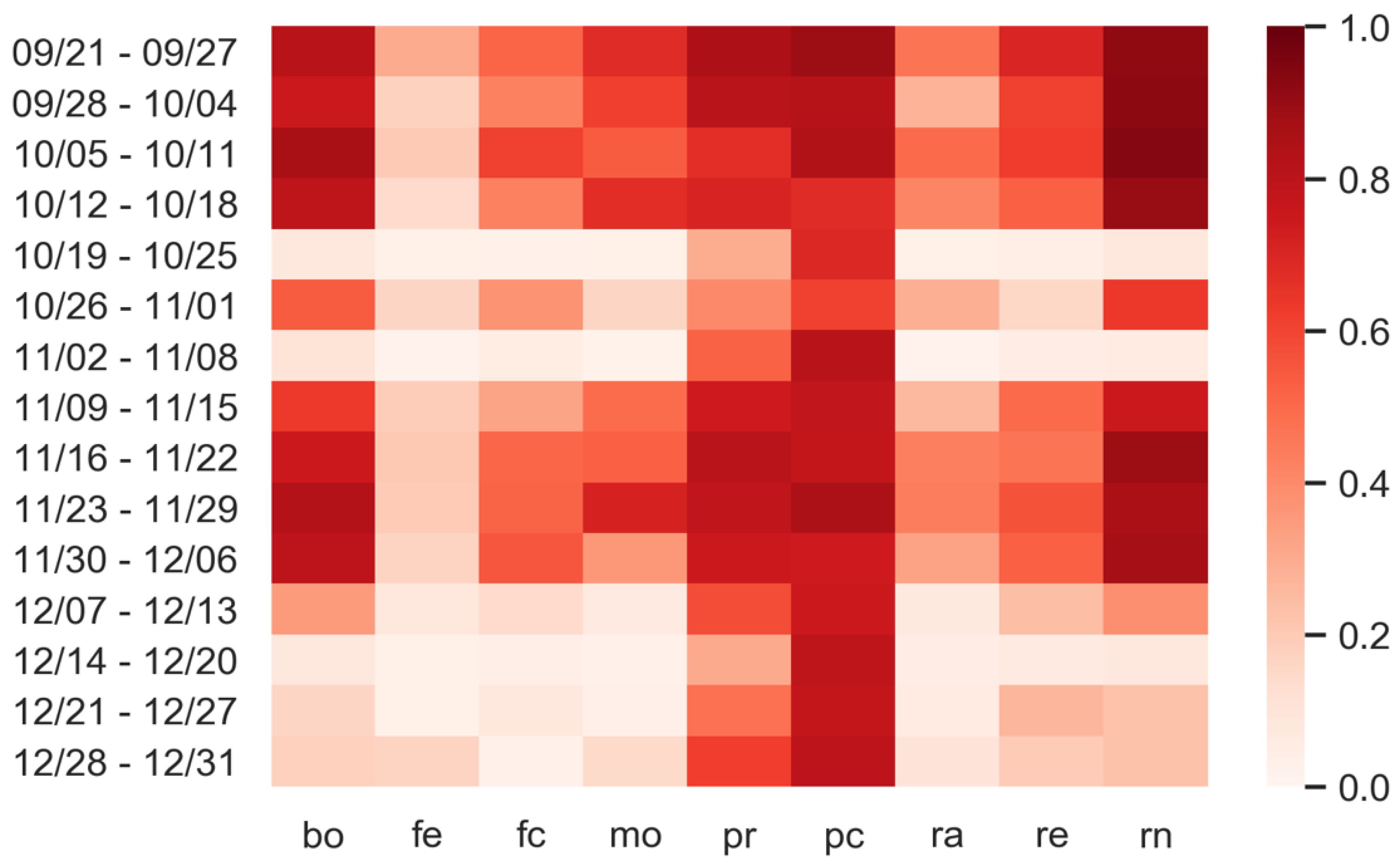
| Day | Bo | Fe | Fc | Mo | Pr | Pc | Ra | Re | Rn |
|---|---|---|---|---|---|---|---|---|---|
| 9/21 | 0.00 | 0.01 | 0.00 | 0.02 | 0.02 | 0.33 | 0.00 | 0.12 | 0.00 |
| 9/22 | 0.00 | 0.03 | 0.00 | 0.12 | 0.05 | 0.12 | 0.02 | 0.04 | 0.00 |
| 9/23 | 0.11 | 0.02 | 0.07 | 0.08 | 0.09 | 0.08 | 0.03 | 0.07 | 0.05 |
| 9/24 | 0.04 | 0.01 | 0.15 | 0.1 | 0.09 | 0.08 | 0.01 | 0.02 | 0.1 |
| 9/25 | 0.00 | 0.02 | 0.00 | 0.06 | 0.06 | 0.06 | 0.01 | 0.02 | 0.00 |
| 9/26 | 0.04 | 0.01 | 0.00 | 0.11 | 0.08 | 0.05 | 0.01 | 0.01 | 0.00 |
| 9/27 | 0.01 | 0.01 | 0.01 | 0.05 | 0.05 | 0.03 | 0.03 | 0.04 | 0.05 |
| 9/28 | 0.00 | 0.03 | 0.00 | 0.12 | 0.04 | 0.09 | 0.03 | 0.06 | 0.00 |
| 9/29 | 0.01 | 0.07 | 0.00 | 0.15 | 0.06 | 0.03 | 0.02 | 0.04 | 0.00 |
| 9/30 | 0.02 | 0.01 | 0.01 | 0.03 | 0.01 | 0.13 | 0.00 | 0.01 | 0.00 |
| 10/1 | 0.00 | 0.01 | 0.00 | 0.26 | 0.05 | 0.07 | 0.04 | 0.04 | 0.00 |
| 10/2 | 0.01 | 0.09 | 0.1 | 0.08 | 0.09 | 0.14 | 0.02 | 0.04 | 0.00 |
| 10/3 | 0.07 | 0.02 | 0.06 | 0.1 | 0.15 | 0.19 | 0.01 | 0.07 | 0.01 |
| 10/4 | 0.14 | 0.03 | 0.11 | 0.22 | 0.24 | 0.15 | 0.02 | 0.03 | 0.12 |
| 10/5 | 0.01 | 0.04 | 0.01 | 0.11 | 0.05 | 0.19 | 0.05 | 0.01 | 0.01 |
| 10/6 | 0.00 | 0.06 | 0.00 | 0.06 | 0.08 | 0.05 | 0.00 | 0.02 | 0.00 |
| 10/7 | 0.00 | 0.00 | 0.02 | 0.12 | 0.4 | 0.12 | 0.01 | 0.09 | 0.00 |
| 10/8 | 0.07 | 0.04 | 0.13 | 0.06 | 0.24 | 0.23 | 0.04 | 0.06 | 0.02 |
| 10/9 | 0.1 | 0.07 | 0.11 | 0.09 | 0.22 | 0.3 | 0.08 | 0.12 | 0.05 |
| 10/10 | 0.03 | 0.07 | 0.01 | 0.22 | 0.19 | 0.19 | 0.03 | 0.06 | 0.01 |
| 10/11 | 0.01 | 0.04 | 0.01 | 0.13 | 0.32 | 0.18 | 0.05 | 0.07 | 0.01 |
| 10/12 | 0.01 | 0.13 | 0.15 | 0.36 | 0.28 | 0.21 | 0.04 | 0.09 | 0.02 |
| 10/13 | 0.00 | 0.01 | 0.03 | 0.04 | 0.26 | 0.04 | 0.05 | 0.07 | 0.00 |
| 10/14 | 0.03 | 0.04 | 0.08 | 0.06 | 0.21 | 0.52 | 0.12 | 0.08 | 0.00 |
| 10/15 | 0.04 | 0.11 | 0.04 | 0.16 | 0.44 | 0.47 | 0.05 | 0.06 | 0.06 |
| 10/16 | 0.07 | 0.08 | 0.23 | 0.37 | 0.51 | 0.34 | 0.05 | 0.12 | 0.04 |
| 10/17 | 0.16 | 0.09 | 0.12 | 0.19 | 0.41 | 0.28 | 0.09 | 0.23 | 0.04 |
| 10/18 | 0.02 | 0.21 | 0.04 | 0.06 | 0.14 | 0.43 | 0.15 | 0.05 | 0.07 |
| 10/19 | 0.03 | 0.47 | 0.05 | 0.22 | 0.67 | 0.35 | 0.11 | 0.6 | 0.23 |
| 10/20 | 0.11 | 0.11 | 0.13 | 0.16 | 0.56 | 0.66 | 0.1 | 0.24 | 0.15 |
| 10/21 | 0.06 | 0.16 | 0.05 | 0.05 | 0.28 | 0.86 | 0.07 | 0.07 | 0.03 |
| 10/22 | 0.05 | 0.09 | 0.13 | 0.1 | 0.38 | 0.82 | 0.07 | 0.07 | 0.03 |
| 10/23 | 0.05 | 0.12 | 0.06 | 0.19 | 0.62 | 0.81 | 0.03 | 0.18 | 0.02 |
| 10/24 | 0.12 | 0.21 | 0.21 | 0.2 | 0.53 | 0.9 | 0.22 | 0.25 | 0.03 |
| 10/25 | 0.34 | 0.27 | 0.11 | 0.18 | 0.36 | 0.92 | 0.1 | 0.19 | 0.07 |
| 10/26 | 0.18 | 0.11 | 0.04 | 0.18 | 0.49 | 0.81 | 0.08 | 0.19 | 0.05 |
| 10/27 | 0.16 | 0.1 | 0.4 | 0.17 | 0.62 | 0.86 | 0.23 | 0.16 | 0.11 |
| 10/28 | 0.27 | 0.18 | 0.26 | 0.15 | 0.59 | 0.85 | 0.28 | 0.22 | 0.19 |
| 10/29 | 0.17 | 0.3 | 0.05 | 0.19 | 0.84 | 0.82 | 0.05 | 0.26 | 0.04 |
| 10/30 | 0.02 | 0.08 | 0.07 | 0.18 | 0.77 | 0.6 | 0.06 | 0.11 | 0.02 |
| 10/31 | 0.04 | 0.27 | 0.25 | 0.13 | 0.4 | 0.64 | 0.14 | 0.12 | 0.01 |
| 11/1 | 0.04 | 0.14 | 0.11 | 0.23 | 0.68 | 0.91 | 0.09 | 0.12 | 0.02 |
| 11/2 | 0.09 | 0.06 | 0.15 | 0.18 | 0.43 | 0.64 | 0.15 | 0.1 | 0.04 |
| 11/3 | 0.07 | 0.47 | 0.14 | 0.2 | 0.33 | 0.7 | 0.25 | 0.21 | 0.04 |
| 11/4 | 0.23 | 0.16 | 0.21 | 0.38 | 0.64 | 0.84 | 0.2 | 0.33 | 0.05 |
| 11/5 | 0.17 | 0.17 | 0.06 | 0.15 | 0.53 | 0.48 | 0.25 | 0.13 | 0.02 |
| 11/6 | 0.03 | 0.02 | 0.04 | 0.15 | 0.62 | 0.35 | 0.04 | 0.03 | 0.01 |
| 11/7 | 0.05 | 0.05 | 0.03 | 0.02 | 0.3 | 0.43 | 0.03 | 0.03 | 0.03 |
| 11/8 | 0.03 | 0.05 | 0.06 | 0.11 | 0.42 | 0.27 | 0.01 | 0.08 | 0.02 |
| 11/9 | 0.02 | 0.07 | 0.03 | 0.28 | 0.68 | 0.23 | 0.02 | 0.05 | 0.03 |
| 11/10 | 0.07 | 0.06 | 0.03 | 0.07 | 0.41 | 0.18 | 0.1 | 0.12 | 0.07 |
| 11/11 | 0.04 | 0.01 | 0.17 | 0.15 | 0.49 | 0.22 | 0.04 | 0.14 | 0.01 |
| 11/12 | 0.06 | 0.09 | 0.05 | 0.28 | 0.67 | 0.07 | 0.04 | 0.18 | 0.05 |
| 11/13 | 0.02 | 0.02 | 0.02 | 0.01 | 0.14 | 0.1 | 0.04 | 0.01 | 0.02 |
| 11/14 | 0.03 | 0.01 | 0.03 | 0.02 | 0.13 | 0.15 | 0.01 | 0.02 | 0.05 |
| 11/15 | 0.01 | 0.02 | 0.01 | 0.08 | 0.47 | 0.1 | 0.02 | 0.05 | 0.05 |
| 11/16 | 0.08 | 0.00 | 0.01 | 0.09 | 0.41 | 0.03 | 0.06 | 0.03 | 0.00 |
| 11/17 | 0.01 | 0.01 | 0.02 | 0.03 | 0.09 | 0.05 | 0.02 | 0.03 | 0.01 |
| 11/18 | 0.01 | 0.09 | 0.03 | 0.16 | 0.22 | 0.03 | 0.02 | 0.05 | 0.01 |
| 11/19 | 0.01 | 0.08 | 0.02 | 0.32 | 0.52 | 0.22 | 0.13 | 0.18 | 0.01 |
| 11/20 | 0.03 | 0.04 | 0.16 | 0.04 | 0.17 | 0.05 | 0.07 | 0.04 | 0.04 |
| 11/21 | 0.05 | 0.02 | 0.08 | 0.21 | 0.44 | 0.18 | 0.05 | 0.01 | 0.09 |
| 11/22 | 0.03 | 0.01 | 0.03 | 0.09 | 0.13 | 0.04 | 0.03 | 0.02 | 0.04 |
| 11/23 | 0.04 | 0.04 | 0.02 | 0.08 | 0.26 | 0.1 | 0.02 | 0.05 | 0.01 |
| 11/24 | 0.01 | 0.04 | 0.03 | 0.16 | 0.4 | 0.13 | 0.02 | 0.07 | 0.00 |
| 11/25 | 0.07 | 0.06 | 0.03 | 0.16 | 0.4 | 0.26 | 0.09 | 0.05 | 0.05 |
| 11/26 | 0.14 | 0.02 | 0.08 | 0.22 | 0.52 | 0.21 | 0.13 | 0.07 | 0.08 |
| 11/27 | 0.05 | 0.06 | 0.04 | 0.15 | 0.15 | 0.19 | 0.06 | 0.04 | 0.05 |
| 11/28 | 0.22 | 0.28 | 0.03 | 0.24 | 0.46 | 0.29 | 0.25 | 0.08 | 0.07 |
| 11/29 | 0.12 | 0.04 | 0.14 | 0.23 | 0.31 | 0.51 | 0.15 | 0.22 | 0.11 |
| 11/30 | 0.48 | 0.15 | 0.15 | 0.13 | 0.19 | 0.38 | 0.23 | 0.11 | 0.15 |
| 12/1 | 0.03 | 0.07 | 0.09 | 0.11 | 0.39 | 0.16 | 0.12 | 0.05 | 0.12 |
| 12/2 | 0.05 | 0.09 | 0.03 | 0.09 | 0.52 | 0.63 | 0.07 | 0.1 | 0.02 |
| 12/3 | 0.04 | 0.04 | 0.03 | 0.04 | 0.32 | 0.67 | 0.03 | 0.05 | 0.04 |
| 12/4 | 0.04 | 0.08 | 0.02 | 0.09 | 0.38 | 0.32 | 0.07 | 0.04 | 0.02 |
| 12/5 | 0.14 | 0.08 | 0.06 | 0.27 | 0.76 | 0.66 | 0.13 | 0.04 | 0.01 |
| 12/6 | 0.14 | 0.08 | 0.22 | 0.1 | 0.38 | 0.5 | 0.12 | 0.06 | 0.07 |
| 12/7 | 0.01 | 0.36 | 0.35 | 0.25 | 0.66 | 0.45 | 0.25 | 0.17 | 0.3 |
| 12/8 | 0.03 | 0.32 | 0.19 | 0.38 | 0.38 | 0.48 | 0.2 | 0.08 | 0.03 |
| 12/9 | 0.15 | 0.22 | 0.03 | 0.13 | 0.35 | 0.55 | 0.2 | 0.08 | 0.01 |
| 12/10 | 0.12 | 0.12 | 0.17 | 0.1 | 0.45 | 0.56 | 0.09 | 0.05 | 0.34 |
| 12/11 | 0.24 | 0.08 | 0.11 | 0.09 | 0.36 | 0.73 | 0.08 | 0.08 | 0.06 |
| 12/12 | 0.1 | 0.06 | 0.04 | 0.18 | 0.22 | 0.77 | 0.09 | 0.05 | 0.03 |
| 12/13 | 0.23 | 0.19 | 0.25 | 0.19 | 0.53 | 0.9 | 0.2 | 0.22 | 0.09 |
| 12/14 | 0.09 | 0.12 | 0.18 | 0.22 | 0.39 | 0.79 | 0.22 | 0.19 | 0.12 |
| 12/15 | 0.15 | 0.27 | 0.18 | 0.24 | 0.72 | 0.84 | 0.23 | 0.26 | 0.07 |
| 12/16 | 0.07 | 0.38 | 0.1 | 0.29 | 0.73 | 0.85 | 0.29 | 0.13 | 0.07 |
| 12/17 | 0.05 | 0.18 | 0.21 | 0.12 | 0.36 | 0.82 | 0.16 | 0.09 | 0.12 |
| 12/18 | 0.12 | 0.18 | 0.08 | 0.26 | 0.53 | 0.86 | 0.18 | 0.18 | 0.05 |
| 12/19 | 0.16 | 0.36 | 0.42 | 0.38 | 0.55 | 0.92 | 0.24 | 0.33 | 0.06 |
| 12/20 | 0.13 | 0.05 | 0.18 | 0.13 | 0.42 | 0.71 | 0.24 | 0.15 | 0.07 |
| 12/21 | 0.18 | 0.28 | 0.33 | 0.2 | 0.51 | 0.71 | 0.27 | 0.34 | 0.17 |
| 12/22 | 0.06 | 0.48 | 0.15 | 0.23 | 0.37 | 0.44 | 0.4 | 0.17 | 0.00 |
| 12/23 | 0.59 | 0.08 | 0.41 | 0.13 | 0.57 | 0.5 | 0.25 | 0.19 | 0.04 |
| 12/24 | 0.12 | 0.14 | 0.14 | 0.08 | 0.43 | 0.66 | 0.1 | 0.08 | 0.15 |
| 12/25 | 0.07 | 0.11 | 0.08 | 0.11 | 0.24 | 0.48 | 0.14 | 0.12 | 0.06 |
| 12/26 | 0.09 | 0.23 | 0.1 | 0.18 | 0.52 | 0.8 | 0.1 | 0.08 | 0.16 |
| 12/27 | 0.1 | 0.1 | 0.11 | 0.18 | 0.49 | 0.82 | 0.11 | 0.16 | 0.2 |
| 12/28 | 0.05 | 0.15 | 0.03 | 0.21 | 0.49 | 0.63 | 0.1 | 0.12 | 0.02 |
| 12/29 | 0.09 | 0.22 | 0.13 | 0.19 | 0.45 | 0.86 | 0.18 | 0.15 | 0.04 |
| 12/30 | 0.27 | 0.22 | 0.19 | 0.13 | 0.27 | 0.7 | 0.15 | 0.12 | 0.1 |
| 12/31 | 0.12 | 0.24 | 0.05 | 0.12 | 0.55 | 0.5 | 0.12 | 0.04 | 0.06 |
© 2020 by the authors. Licensee MDPI, Basel, Switzerland. This article is an open access article distributed under the terms and conditions of the Creative Commons Attribution (CC BY) license (http://creativecommons.org/licenses/by/4.0/).
Share and Cite
Mirri, S.; Delnevo, G.; Roccetti, M. Is a COVID-19 Second Wave Possible in Emilia-Romagna (Italy)? Forecasting a Future Outbreak with Particulate Pollution and Machine Learning. Computation 2020, 8, 74. https://0-doi-org.brum.beds.ac.uk/10.3390/computation8030074
Mirri S, Delnevo G, Roccetti M. Is a COVID-19 Second Wave Possible in Emilia-Romagna (Italy)? Forecasting a Future Outbreak with Particulate Pollution and Machine Learning. Computation. 2020; 8(3):74. https://0-doi-org.brum.beds.ac.uk/10.3390/computation8030074
Chicago/Turabian StyleMirri, Silvia, Giovanni Delnevo, and Marco Roccetti. 2020. "Is a COVID-19 Second Wave Possible in Emilia-Romagna (Italy)? Forecasting a Future Outbreak with Particulate Pollution and Machine Learning" Computation 8, no. 3: 74. https://0-doi-org.brum.beds.ac.uk/10.3390/computation8030074