Non-Intrusive In-Plane-Out-of-Plane Separated Representation in 3D Parametric Elastodynamics

Abstract

Mesh-based solution of 3D models defined in plate or shell domains remains a challenging issue nowadays due to the fact that the needed meshes generally involve too many degrees of freedom. When the considered problem involves some parameters aiming at computing its parametric solution the difficulty is twofold. The authors proposed, in some of their former works, strategies for solving both, however they suffer from a deep intrusiveness. This paper proposes a totally novel approach that from any existing discretization is able to reduce the 3D parametric complexity to the one characteristic of a simple 2D calculation. Thus, the 3D complexity is reduced to 2D, the parameters included naturally into the solution, and the procedure applied on a discretization performed with a standard software, which taken together enable real-time engineering.

1. Introduction

The finite element method (FEM) remains the major protagonist of SBE (Simulation Based Engineering). It is largely considered for performing three-dimensional (3D) analyses, however the number of degrees of freedom that certain models involve compromises the solution efficiency. That is the case of problems defined in plate or shell domains, where the mesh size is almost determined by the domain thickness and the material and/or solution details to be represented.

The enormous number of degrees of freedom that such models involve makes the use of traditional discretization techniques difficult. A possibility to circumvent such difficulty consists of reducing the model complexity. In this sense simplified descriptions can be derived by introducing adequate kinematic and mechanic hypotheses, leading to usual shell, plate or beam theories.

However, when inelastic behaviors occur, some of them implying localization, or for complex microstructures (e.g., foams or architectured materials and metamaterials), usual hypotheses fail, and the 3D descriptions become compulsory locally or globally.

Another valuable route proposed in our former works relies on the use of separated representations within the Proper Generalized Decomposition (PGD) framework. The interested reader can refer to [1] for a primer and [2] for the use of PGD in the solution of parametrized problems. As PGD considers a separated representation of the solution, the computational complexity reduces to the one of the variables involved in the separated form. Thus, if a generic problem involving the unknown field $u(x,y,z)$ is defined in a hexahedral domain, one is tempted to express the problem solution in the separated form

$$u(x,y,z)\approx \sum _{i=1}^N{X}_i\left(x\right)Y_i\left(y\right)Z_i\left(z\right),$$

(1)

and consequently the complexity reduces from the one characteristic of a 3D problem to the one characteristic of the 1D solutions involved in the determination of functions $X_i\left(x\right)$, $Y_i\left(y\right)$ and $Z_i\left(z\right)$.

When the problem is defined in a plate (or shell) domain $\Omega ={\Omega }_{xy}\times {\Omega }_z$, with ${\Omega }_{xy}\subset {\mathbb{R}}^2$ and ${\Omega }_z=(0,H)$, the 3D solution can be expressed from

$$u(x,y,z)\approx \sum _{i=1}^N{X}_i(x,y)Z_i\left(z\right),$$

(2)

and now the complexity reduces to the one associated with the solution of the 2D problems for determining functions $X_i(x,y)$, the computational complexity being related to the calculation of the one-dimensional functions $Z_i\left(z\right)$ negligible with respect to the former.

When considering vector-valued fields, as the displacement field in the mechanical problems later addressed, it reads

$$\mathbf{u}(\mathit{x},\mathit{y},\mathit{z})\approx \sum _{i=1}^N{\mathbf{X}}^i\left(\mathit{x}\right)\circ {\mathbf{Y}}^i\left(\mathit{y}\right)\circ {\mathbf{Z}}^i\left(\mathit{z}\right)$$

(3)

where “∘” stands for Hadamard product (component to component), with $\Omega ={\Omega }_x\times {\Omega }_y\times {\Omega }_z$.

The in-plane-out-of-plane separated representation of the displacement field defined in a plate domain reads

$$\mathbf{u}(\mathit{x},\mathit{y},\mathit{z})\approx \sum _{i=1}^N{\mathbf{X}}^i(\mathit{x},\mathit{y})\circ {\mathbf{Z}}^i\left(\mathit{z}\right)$$

(4)

with $\Omega ={\Omega }_{xy}\times {\Omega }_z$.

In-plane-out-of-plane separated representations have been applied to solve elastic problems defined in plate [3], shell [4], extruded domains [5], multilayered composite structures [6,7], and were extended to cover many other physics: the solution of thermal problems [8]; the solution of the Navier–Stokes equations [9] and the simulation of heat and mass transfer [10]; the squeeze flows of Newtonian and non-Newtonian fluids in laminates in [11], among may others.

However, the just referred separated representation becomes strongly intrusive with respect to existing structural mechanics softwares. In a recent work [12], authors proposed a variant, able to reduce the computational complexity as well as its implementation intrusiveness. For that purpose, instead of the usual process of applying variables separation and then proceeding to the problem discretization, authors proposed to discretize, in a usual FEM sense, and then enforce the variable separation for solving the algebraic system resulting from the discretization.

The objective of this paper is to move a step forward, to extend such a non-intrusive approach to parametric elastodynamics, where the real-time evaluation of the structure response for any possible loading, while considering the structure or the material composing it, defined from a series of parameters, constitutes an excellent tool for enabling safer designs as well as for real-time motoring and active control. The real-time evaluation of dynamical responses is possible as soon as a parametric solution of it, involving parameters describing the structure, the materials composing it and the loading, is available. In the preset work, that parametric solution is computed in a non-intrusive manner, by using any well experienced numerical discretization method and commercial solver.

The paper is organized as follows: Section 2 revisits the non-intrusive formulation of the in-plane-out-of-plane separated representation, that allows reducing the computational complexity as well as the intrusiveness of the standard PGD procedure. In Section 3, the non-intrusive formulation is implemented to address parametric elastodynamics. Section 4 proves the benefits of the proposed approach through a numerical example, before addressing the main conclusions of the work in the last section.

2. Methods

2.1. Non-Intrusive Formulation of the In-Plane-Out-of-Plane Separated Representation

In what follows the in-plane-out-of-plane decomposition for solving 3D problems based on a non-intrusive approach is cosidered. The domain is expressed from $\Omega ={\Omega }_{xy}\times {\Omega }_z$ with $(x,y)$∈${\Omega }_{xy}$ and z∈${\Omega }_z=(0,H)$, and the separated representation of the displacement field $\mathbf{u}=(\mathit{u},\mathit{v},\mathit{w})$ reads

$$\mathbf{u}(\mathit{x},\mathit{y},\mathit{z})\approx \left(\begin{array}{c}\mathit{u}(\mathit{x},\mathit{y},\mathit{z})\\ \mathit{v}(\mathit{x},\mathit{y},\mathit{z})\\ \mathit{w}(\mathit{x},\mathit{y},\mathit{z})\end{array}\right)=\sum _{k=1}^N\left(\begin{array}{c}{\mathcal{X}}_u^k(\mathit{x},\mathit{y})·{\mathcal{Z}}_u^k\left(\mathit{z}\right)\\ {\mathcal{X}}_v^k(\mathit{x},\mathit{y})·{\mathcal{Z}}_v^k\left(\mathit{z}\right)\\ {\mathcal{X}}_w^k(\mathit{x},\mathit{y})·{\mathcal{Z}}_w^k\left(\mathit{z}\right)\end{array}\right)$$

$$=\sum _{k=1}^N{\mathbf{X}}^k(\mathit{x},\mathit{y})\circ {\mathbf{Z}}^k\left(\mathit{z}\right),$$

(5)

where vectors ${\mathbf{X}}^k$ are composed by the functions involving the in-plane coordinates $(x,y)$ while ${\mathbf{Z}}^k$ involves the thickness coordinate $\left(z\right)$. This formulation seems again the most appealing route for addressing 3D discretizations while keeping the computational complexity the one characteristic of 2D discretizations. However, the use of the above separated representation into the discretization process results in a very intrusive formulation. A new alterative formulation is proposed in what follows.

The elasto-static problem, within a fully 3D finite element formulation, leads to the algebraic system

$$\mathbf{K}\mathbf{U}=\mathbf{F},$$

(6)

where $\mathbf{F}$ is the vector grouping the nodal loads, $\mathbf{K}$ is the stiffness matrix and $\mathbf{U}$ contains the nodal displacements.

Now, a layered mesh is cosidered, composed of $\mathcal{L}$ layers along the thickness, with $l=1,\dots ,\mathcal{L}$, each containing m nodes (defining the mesh of ${\Omega }_{xy}$). The nodal displacements vector on layer l, ${\mathbf{U}}_l$, is expressed from

$${\mathbf{U}}_l={\left[u_{1,l},u_{2,l},\dots ,u_{m,l},v_{1,l},v_{2,l},\dots v_{m,l},w_{1,l},w_{2,l},\dots ,w_{m,l}\right]}^T.$$

(7)

Thus, Equation (6) can be rewritten in the form

$$\left(\begin{array}{cccc}{\mathbf{K}}_{11}& {\mathbf{K}}_{12}& \cdots & {\mathbf{K}}_{1\mathcal{L}}\\ {\mathbf{K}}_{21}& {\mathbf{K}}_{22}& \cdots & {\mathbf{K}}_{2\mathcal{L}}\\ ⋮& ⋮& \ddots & ⋮\\ {\mathbf{K}}_{\mathcal{L}1}& {\mathbf{K}}_{\mathcal{L}2}& \cdots & {\mathbf{K}}_{\mathcal{L}\mathcal{L}}\end{array}\right)\left(\begin{array}{c}{\mathbf{U}}_1\\ {\mathbf{U}}_2\\ ⋮\\ {\mathbf{U}}_{\mathcal{L}}\end{array}\right)=\left(\begin{array}{c}{\mathbf{F}}_1\\ {\mathbf{F}}_2\\ ⋮\\ {\mathbf{F}}_{\mathcal{L}}\end{array}\right),$$

(8)

with the associated nodal forces written by

$${\mathbf{F}}_l={\left[F_{1,l}^x,F_{2,l}^x,\cdots ,F_{m,l}^x,F_{1,l}^y,F_{2,l}^y,\cdots ,F_{m,l}^y,F_{1,l}^z,F_{2,l}^z,\cdots ,F_{m,l}^z\right]}^T.$$

(9)

2.2. Separated Representation Constructor

Now, taking into account the in-plane-out-of-plane separated representation given in Equation (5), the layer displacements read

$${\mathbf{U}}_l\approx \sum _{k=1}^N\left(\begin{array}{c}{\mathcal{P}}_u^k·{\mathcal{T}}_{u,l}^k\\ {\mathcal{P}}_v^k·{\mathcal{T}}_{v,l}^k\\ {\mathcal{P}}_w^k·{\mathcal{T}}_{w,l}^k\end{array}\right)=\sum _{k=1}^N{\mathbf{P}}^k\circ {\mathbf{T}}_l^k,$$

(10)

where

$$\left\{\begin{array}{c}{\mathcal{P}}_u^k={\left[P_{u,1}^k,P_{u,2}^k,\dots ,P_{u,m}^k\right]}^T\hfill \\ {\mathcal{P}}_v^k={\left[P_{v,1}^k,P_{v,2}^k,\dots ,P_{v,m}^k\right]}^T\hfill \\ {\mathcal{P}}_w^k={\left[P_{w,1}^k,P_{w,2}^k,\dots ,P_{w,m}^k\right]}^T\hfill \end{array}\right.,$$

(11)

with ${\mathbf{P}}^k={\left[{\mathcal{P}}_u^{k^T},{\mathcal{P}}_v^{k^T},{\mathcal{P}}_w^{k^T}\right]}^T$.

At its turn,

$$\left\{\begin{array}{c}{\mathcal{T}}_{u,l}^k=T_{u,l}^k{\left[1,1,\dots ,1\right]}^T=T_{u,l}^k{\mathbf{I}}_m^T\hfill \\ {\mathcal{T}}_{v,l}^k=T_{v,l}^k{\left[1,1,\dots ,1\right]}^T=T_{v,l}^k{\mathbf{I}}_m^T\hfill \\ {\mathcal{T}}_{w,l}^k=T_{w,l}^k{\left[1,1,\dots ,1\right]}^T=T_{w,l}^k{\mathbf{I}}_m^T\hfill \end{array}\right.,$$

(12)

with ${\mathbf{I}}_m$ the vector with m unitary entries and ${\mathbf{T}}_l^k={\left[{\mathcal{T}}_{u,l}^{k^T},{\mathcal{T}}_{v,l}^{k^T},{\mathcal{T}}_{w,l}^{k^T}\right]}^T$.

Now, it is assumed that at the n enrichment step, ${\mathbf{U}}^{n-1}$ is already known, and that now the algorithm looks for the solution ${\mathbf{U}}^n$, that at each layer $l=1,\dots ,\mathcal{L}$ reads

$${\mathbf{U}}_l^n={\mathbf{U}}_l^{n-1}+{\mathbf{P}}^n\circ {\mathbf{T}}_l^n=\sum _{k=1}^{n-1}{\mathbf{P}}^k\circ {\mathbf{T}}_l^k+{\mathbf{P}}^n\circ {\mathbf{T}}_l^n.$$

(13)

2.2.1. In-Plane Update

When looking for the in-plane update, Equation (13) can be expressed as

$${\mathbf{U}}_l^n=\sum _{k=1}^{n-1}{\mathbb{Z}}_l^k{\mathbf{P}}^k+{\mathbb{Z}}_l^n{\mathbf{P}}^n$$

(14)

with ${\mathbb{Z}}_l^j=diag\left({\mathbf{T}}_l^j\right)$, for $j=1,\dots ,n$.

Thus, the nodal displacements vector ${\mathbf{U}}^n$ reads

$${\mathbf{U}}^n=\sum _{k=1}^{n-1}{\mathbb{T}}^k{\mathbf{P}}^k+{\mathbb{T}}^n{\mathbf{P}}^n$$

(15)

with ${\mathbb{T}}^j={[{\mathbb{Z}}_1^j,\dots ,{\mathbb{Z}}_{\mathcal{L}}^j]}^T$.

Now, premultiplying Equation (6) by the transpose of the test function ${\mathbf{U}}^{*}={\mathbb{T}}^n{\mathbf{P}}^{*}$, and introducing Equation (15), it results

$${\mathbf{P}}^{{*}^T}\left[{\mathbb{T}}^{n^T}\mathbf{K}{\mathbb{T}}^n\right]{\mathbf{P}}^n={\mathbf{P}}^{{*}^T}{\mathbb{T}}^{n^T}\mathbf{F}-{\mathbf{P}}^{{*}^T}{\mathbb{T}}^{n^T}\mathbf{K}\left(\sum _{k=1}^{n-1}{\mathbb{T}}^k{\mathbf{P}}^k\right),$$

(16)

that, ${\mathbf{P}}^{{*}^T}$ being arbitrary, leads finally to the linear system

$$\left[{\mathbb{T}}^{n^T}\mathbf{K}{\mathbb{T}}^n\right]{\mathbf{P}}^n={\mathbb{T}}^{n^T}\mathbf{F}-{\mathbb{T}}^{n^T}\mathbf{K}\left(\sum _{k=1}^{n-1}{\mathbb{T}}^k{\mathbf{P}}^k\right).$$

(17)

This procedure allows to compute vector ${\mathbf{P}}^n$ from ${\mathbb{T}}^n$, by solving the linear system associated with the in-plane 2D problem (17).

2.2.2. Through-The-Thickness Update

As soon as ${\mathbf{P}}^n$ is available, $T_{u,l}^n$, $T_{v,l}^n$ and $T_{w,l}^n$ must be computed, for $l=1,\dots ,\mathcal{L}$. For this purpose, we first define matrices ${\mathbb{P}}^j=diag\left({\mathbf{P}}^j\right)$, $j=1,\dots ,n$, vectors ${\mathbf{T}}^j={\left[T_{u,1}^j,T_{v,1}^j,T_{w,1}^j,\dots ,T_{u,\mathcal{L}}^j,T_{v,\mathcal{L}}^j,T_{w,\mathcal{L}}^j\right]}^T$ and the m-components vectors ${\mathbf{O}}_m={\left[0,\dots ,0\right]}^T$ and ${\mathbf{I}}_m={\left[1,\dots ,1\right]}^T$ that at its turn allows defining the $m\times 3$ matrix $\mathbf{C}$

$$\mathbf{C}=\left(\begin{array}{ccc}{\mathbf{I}}_m& {\mathbf{O}}_m& {\mathbf{O}}_m\\ {\mathbf{O}}_m& {\mathbf{I}}_m& {\mathbf{O}}_m\\ {\mathbf{O}}_m& {\mathbf{O}}_m& {\mathbf{I}}_m\end{array}\right),$$

(18)

such that the following relation applies

$${\mathbf{U}}_l\approx \sum _{k=1}^N{\mathbb{P}}^k\mathbf{C}\left(\begin{array}{c}{T}_{u,l}^k\\ T_{v,l}^k\\ T_{w,l}^k\end{array}\right).$$

(19)

By defiining ${\tilde{\mathbb{P}}}^k={\mathbb{P}}^k\mathbf{C}$, and then the block diagonal matrix ${\mathfrak{P}}^k$ from

$${\mathfrak{P}}^k=\left(\begin{array}{ccc}{\tilde{\mathbb{P}}}^k& \mathbf{0}& \cdots \\ \mathbf{0}& {\tilde{\mathbb{P}}}^k& \cdots \\ ⋮& ⋮& \ddots \end{array}\right),$$

(20)

the global displacement reads

$$\mathbf{U}\approx \sum _{k=1}^N{\mathfrak{P}}^k{\mathbf{T}}^k.$$

(21)

At the enrichment step n, the separated representation of the displacement field reads

$${\mathbf{U}}^n=\sum _{k=1}^{n-1}{\mathfrak{P}}^k{\mathbf{T}}^k+{\mathfrak{P}}^n{\mathbf{T}}^n.$$

(22)

Now, with the test function given by

$${\mathbf{U}}^{*}={\mathfrak{P}}^n{\mathbf{T}}^{*},$$

(23)

premultiplying Equation (6) by the transposition of Equation (23) and using Equation (22), it results

$${\mathbf{T}}^{{*}^T}\left[{\mathfrak{P}}^{n^T}\mathbf{K}{\mathfrak{P}}^n\right]{\mathbf{T}}^n={\mathbf{T}}^{{*}^T}{\mathfrak{P}}^{n^T}\mathbf{F}-{\mathbf{T}}^{{*}^T}{\mathfrak{P}}^{n^T}\mathbf{K}\left(\sum _{k=1}^{n-1}{\mathfrak{P}}^k{\mathbf{T}}^k\right),$$

(24)

that due to the arbitrariness of ${\mathbf{T}}^{*}$, it reduces to

$$\left[{\mathfrak{P}}^{n^T}\mathbf{K}{\mathfrak{P}}^n\right]{\mathbf{T}}^n={\mathfrak{P}}^{n^T}\mathbf{F}-{\mathfrak{P}}^{n^T}\mathbf{K}\left(\sum _{k=1}^{n-1}{\mathfrak{P}}^k{\mathbf{T}}^k\right),$$

(25)

whose computational complexity scales with the number of nodes along the thickness.

Thus, the three-dimensional solution reduces to a sequence of two problems, the ones to compute vectors ${\mathbf{P}}^k$, with a complexity characteristic of 2D discretizations, and the one related to the calculation of vectors ${\mathbf{T}}^k$, whose complexity as just mentioned, is the one characteristic on a 1D discretization, both making use of the standard FEM discrete form guaranteeing its minimal intrusiveness.

3. Problem Formulation

Non-Intrusive Parametric Elastodynamics in Layered Media

Let us consider the general discrete form of linear elastodynamics [13],

$$\mathbf{M}\ddot{\mathbf{U}}\left(t\right)+\mathbf{C}\dot{\mathbf{U}}\left(t\right)+\mathbf{K}\mathbf{U}\left(t\right)=\mathbf{F}\left(t\right)$$

(26)

where $\mathbf{M}$ is the mass matrix, $\ddot{\mathbf{U}}$ is the acceleration vector, $\mathbf{C}$ is the damping matrix, $\dot{\mathbf{U}}$ is the velocity vector, $\mathbf{K}$ is the stiffness matrix, $\mathbf{U}$ is the displacement vector and $\mathbf{F}$ is the external force vector.

Addressing fast transient dynamics can usually be accomplished using explicit integrations that require satisfying stability conditions affecting the largest integration time-step $\Delta t_{\mathrm{m}ax}$, closely related to the size of the elements involved in the mesh $\mathcal{M}$ covering the domain $\Omega$. Many robust integration schemas exist and are widely employed, from the very popular Newmark [14] to more advanced schemes able to preserve inherent mechanical properties [15].

In the context of model order reduction (MOR), in [16] authors proposed a POD-based reduced order modeling (Proper Orthogonal Decomposition) operating in the time domain. Ladeveze and coworkers proposed an extension of their radial approximation [17] for addressing mid-frequency dynamics, the so-called variational theory of complex rays [18].

If damping vanishes, i.e., $\mathbf{C}=\mathbf{0}$ (if it is not the case, it is usually assumed to be proportional, $\mathbf{C}=a_0\mathbf{M}+a_1\mathbf{K}$), and by moving to the frequency-domain through the Fourier transform $\mathcal{F}(•)$, and by denoting $\mathbf{f}\left(\omega \right)=\mathcal{F}\left(\mathbf{F}\right(t\left)\right)$ and $\mathfrak{A}\left(\omega \right)=\mathcal{F}\left(\mathbf{U}\right(t\left)\right)$, Equation (26) reduces to

$$-{\omega }^2\mathbf{M}\mathfrak{A}\left(\omega \right)+\mathbf{K}\mathfrak{A}\left(\omega \right)=\mathbf{f}\left(\omega \right).$$

(27)

In what follows a layered medium consisting of $\mathcal{H}$ material layers is cosidered, with a material property $\mu$ varying from layer to layer, e.g., the elastic modulus, affecting only the stiffness matrix. In these circumstances the global stiffness matrix can be expressed as

$$\mathbf{K}({\mu }_1,\dots ,{\mu }_{\mathcal{H}})={\mu }_1{\mathbf{K}}_1+\cdots +{\mu }_{\mathcal{H}}{\mathbf{K}}_{\mathcal{H}},$$

(28)

and the dynamical problem reads

$$-{\omega }^2\mathbf{M}\mathfrak{A}\left(\omega \right)+\{{\mu }_1{\mathbf{K}}_1+\cdots +{\mu }_{\mathcal{H}}{\mathbf{K}}_{\mathcal{H}}\}\mathfrak{A}\left(\omega \right)=\mathbf{f}\left(\omega \right),$$

(29)

from which one is tempted to look for a general parametric solution in the form $\mathfrak{A}(\omega ,{\mu }_1,\dots ,{\mu }_{\mathcal{H}})$.

The problem weighted residual form reads

$${\int }_{\Gamma }{\mathfrak{A}}^{{*}^T}\left(-{\omega }^2\mathbf{M}+{\mu }_1{\mathbf{K}}_1+\cdots +{\mu }_{\mathcal{H}}{\mathbf{K}}_{\mathcal{H}}\right)\mathfrak{A}d\Gamma ={\int }_{\Gamma }{\mathfrak{A}}^{{*}^T}\mathbf{f}d\Gamma ,$$

(30)

with $\Gamma ={\Omega }_{\omega }\times {\Omega }_{{\mu }_1}\times \cdots \times {\Omega }_{{\mu }_{\mathcal{H}}}$.

Following the rationale described in the previous section, the parametric in-plane-out-of-plane separated representation concerns:

• The in-plane update at the enrichment step n uses

  $${\mathfrak{A}}^n=\sum _{k=1}^{n-1}{\mathbb{T}}^k{\mathbf{P}}^k{W}_k\left(\omega \right){\mathcal{M}}_k^1\left({\mu }_1\right)\cdots +{\mathbb{T}}^n{\mathbf{P}}^n{W}_n\left(\omega \right){\mathcal{M}}_n^1\left({\mu }_1\right)\dots ,$$

  (31)

  with everything known except ${\mathbf{P}}^n$.
  By introducing the approximation (31) and its associated test function into Equation (30) (after this last is integrated into $\Gamma$) and taking into account the arbitrariness of ${\mathbf{P}}^{*}$ the algebraic equation to compute ${\mathbf{P}}^n$ is derived.
• The through-the-thickness update at the enrichment step n uses

  $${\mathfrak{A}}^n=\sum _{k=1}^{n-1}{\mathfrak{P}}^k{\mathbf{T}}^k{W}_k\left(\omega \right){\mathcal{M}}_k^1\left({\mu }_1\right)\cdots +{\mathfrak{P}}^n{\mathbf{T}}^n{W}_n\left(\omega \right){\mathcal{M}}_n^1\left({\mu }_1\right)\dots ,$$

  (32)

  with everything known except ${\mathbf{T}}^n$.
  By introducing the approximation (32) and its associated test function into Equation (30) (after this last is integrated into $\Gamma$) and taking into account the arbitrariness of ${\mathbf{T}}^{*}$, the algebraic equation to compute ${\mathbf{T}}^n$ is defined.
• Parametric update. In this case in Equation (32) everything is known except one of the functions depending on the frequency $W_n\left(\omega \right)$ or the parameters ${\mathcal{M}}_n^h\left({\mu }_h\right)$, $h=1,\dots ,\mathcal{H}$. Introduced into Equation (30) (after this last is integrated into all the variables except the one in which the unknown function is defined) and taking into account the arbitrariness of the associated test function, a scalar algebraic equation that allows calculating the searched function, is obtained.

The fact of including the frequency into the parametric solution has enormous benefits. Thus, after computing the parametric solution, very efficiently because of the reduction complexity from the 3D to the 2D while including the parameters, now, as soon as the loading is known, the FFT (Fast Fourier Transform) applies to compute the frequency content, and with the solution known for each frequency and the problem being linear (the nonlinear case needs an specific treatment [19]), the solution can be reconstructed by simple superposition, for any given material parameter, in real-time.

4. Numerical Example

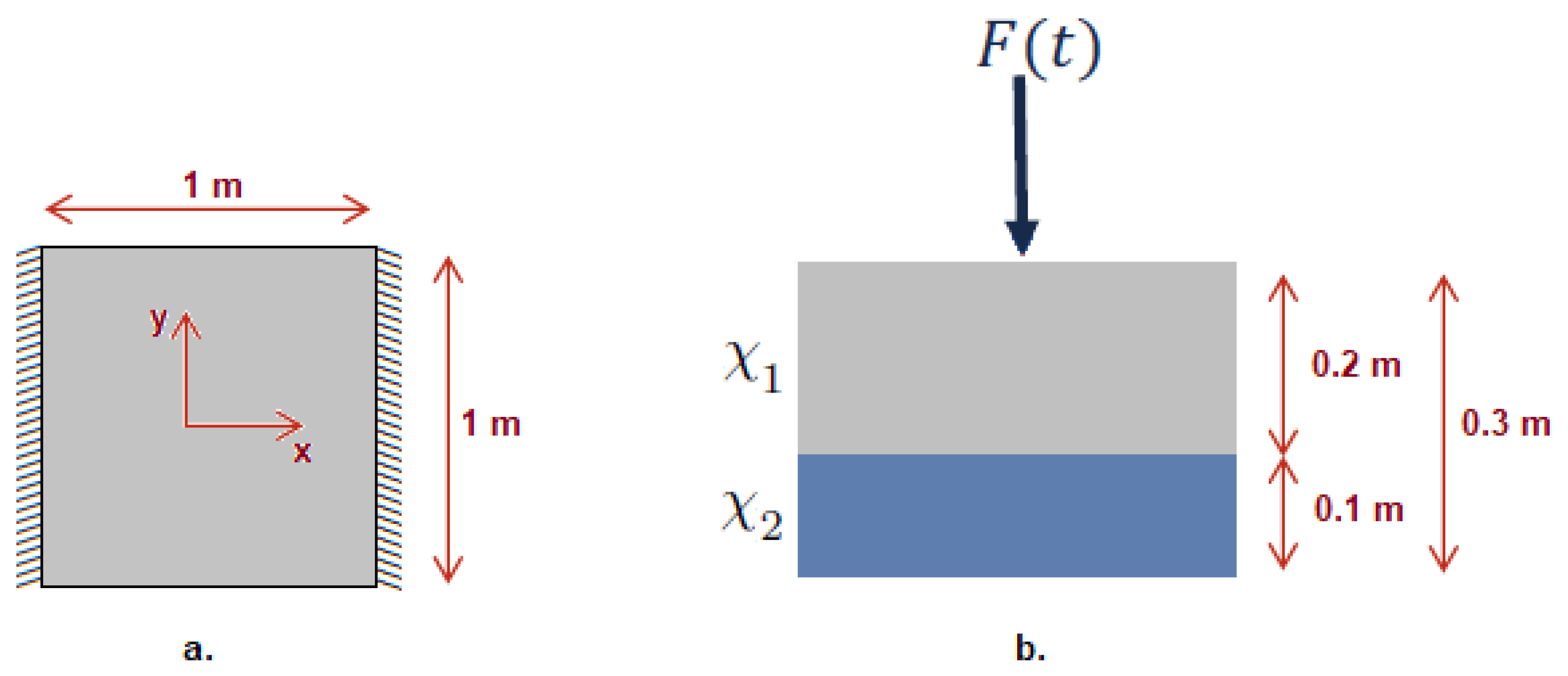
The numerical simulation addressed here considers the separated representation just discussed in the two layers laminate sketched in Figure 1 (with the layers described by the characteristic functions ${\chi }_1$ and ${\chi }_2$), of elastic modulus ${\mu }_1$ and ${\mu }_2$, with the material density given by ${\rho }_1={\rho }_2=1900$ kg/m${}^3$ and the Poisson coefficient ${\nu }_1={\nu }_2=0.1$.

The procedure described in the previous section is applied to calculate the parametric solution of the displacement field ${\mathfrak{A}}^n(\omega ,{\mu }_1,{\mu }_2)$. The parametric domain is defined by ${\Omega }_{\omega }=2\pi (0,25)$s${}^{-1}$, ${\Omega }_{{\mu }_1}=(2\times {10}^8,2\times {10}^9)$ Pa and ${\Omega }_{{\mu }_2}=(2\times {10}^8,2\times {10}^9)$ Pa. The choice of the material parameters aims at representing usual elastic materials, mainly described by their elastic modulus, and concerning the frequency, including it as an extra-coordinate, as previously indicated, enables the real-time calculation of the structural response to any loading (the frequency interval corresponds to the usual spectral content of a dynamical loading, larger intervals will be considered later for approaching the spectral content of a typical earthquake).

The different domains ${\Omega }_{xy}$, ${\Omega }_z$, ${\Omega }_{\omega }$, ${\Omega }_{{\mu }_1}$ and ${\Omega }_{{\mu }_2}$ were discretized by considering respectively 100, 30, 500, 200 and 200 nodes. It is important to recall that a fully mesh-based solution of the 6D problem will imply $6\times {10}^{10}$ nodes, almost unreachable by using reasonable computational availabilities nowadays.

As previously indicated, the fact of computing such a parametric solution allows the analysis of many possible scenarios concerning the material properties of the different structure layers, and the fact of including the frequency makes reconstructing the structural response from the Fourier transform of the applied load possible (very fast when using the Fast Fourier Transform), then the superposition principle applies as the problem is linear. Thus, the solution in the frequency domain results from the frequency-dependent parametric solution weighted with the frequency content of the applied load. Then, the inverse Fourier applies to the superposed response to obtain the fully 3D solution in the time domain. In our knowledge, such a real-time parametric analysis becomes almost impossible when using alternative discetization procedures, justifying the use of the technique proposed here.

The parametric solution computed using the procedure just indicated was compared with the reference one, that as previously indicated consists of the one calculated by using a well experienced time-integration (Newmark) for different values of the material parameters and the applied loads. These solutions computed by standard procedures are quite expensive from a computational point of view, making their use for real-time applications impossible, but allowed to confirm the excellent accuracy of the parametric solution obtained by the methodology presented here.

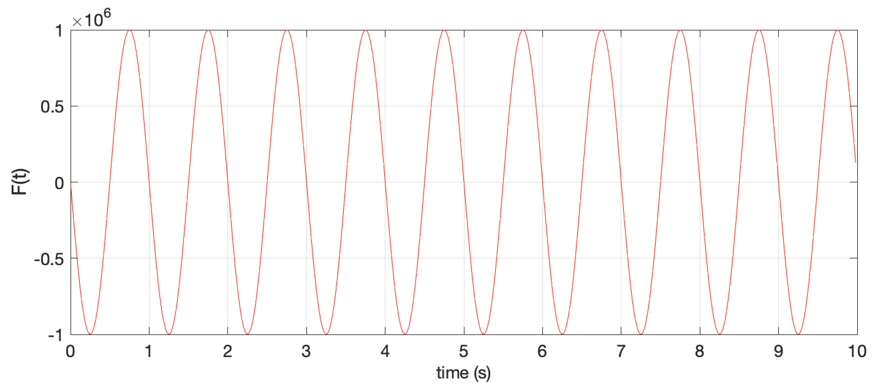
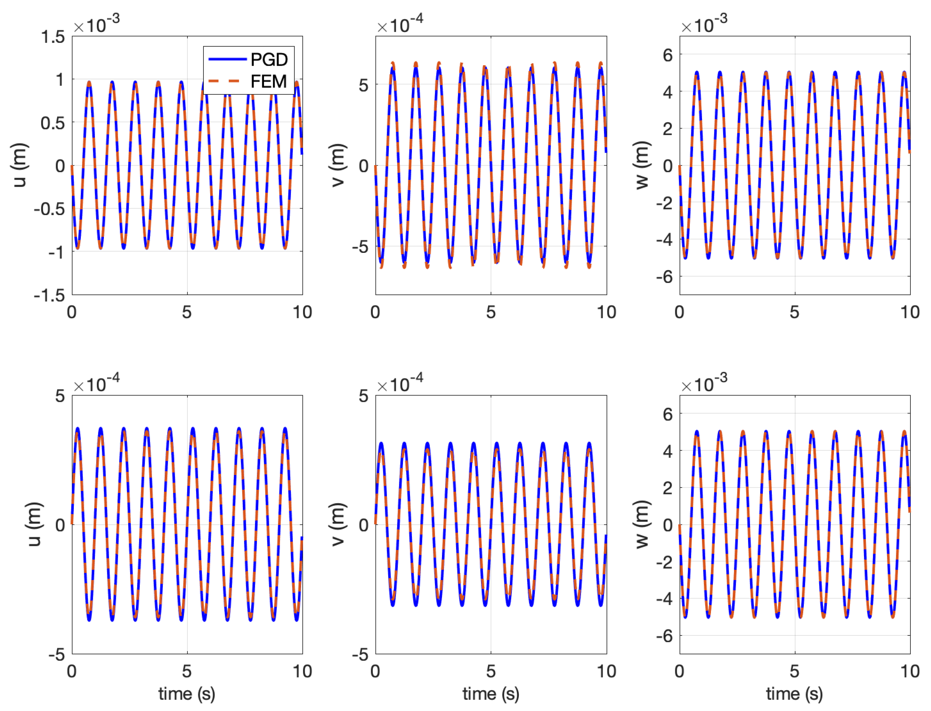
The force, which is applied at the center of the in-plane domain, is depicted in Figure 2. Figure 3 illustrates the time evolution of the displacement field (u, v, w) at the mid-depth of each layer with the in-plane coordinates given by $(0.3,0.3)$ when considering ${\mu }_1=4\times {10}^8$ Pa and ${\mu }_2=1\times {10}^9$ Pa. It also compares the parametric elastodynamics solution with a standard fully three-dimensional finite element time integration for that choice of the parameters, that is considered as reference. A perfect agreement between both solutions can be noticed.

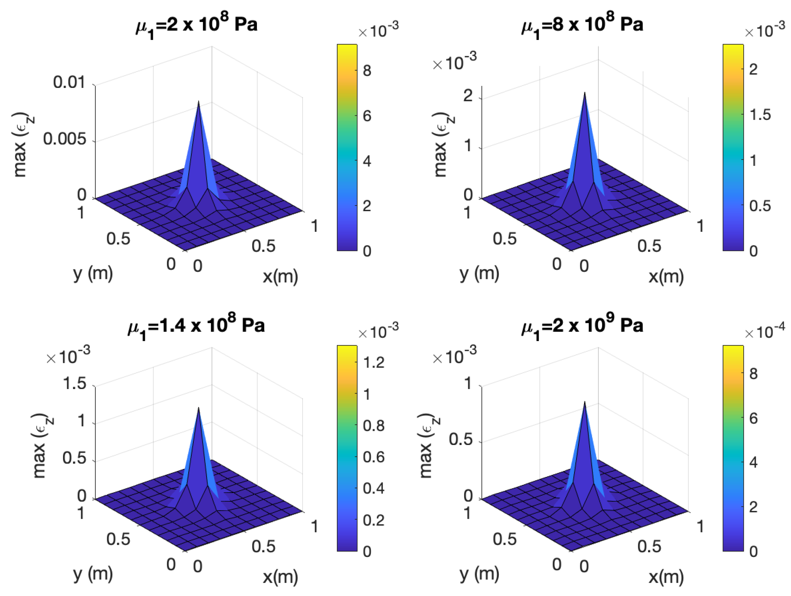
Figure 4 shows the maximum strain ${ϵ}_z$ at the top layer for different values of the elastic modulus ${\mu }_1$ and with ${\mu }_2=2\times {10}^8$ Pa. As expected, the higher the elastic modulus, the smaller the maximum strain. This parametric solution is very useful for the analysis of materials sequencing in laminates, for example in order to optimize the materials sequencing with respect to a certain quantity of interest. PGD enables a significant computing time saving in the solution of parametric models, and in the present case the procedure has an additional benefit due to the in-plane-out-of plane decomposition that allows considering the solution of high-resolved 3D models at the cost of usual 2D solutions, gains that were reported in [3].

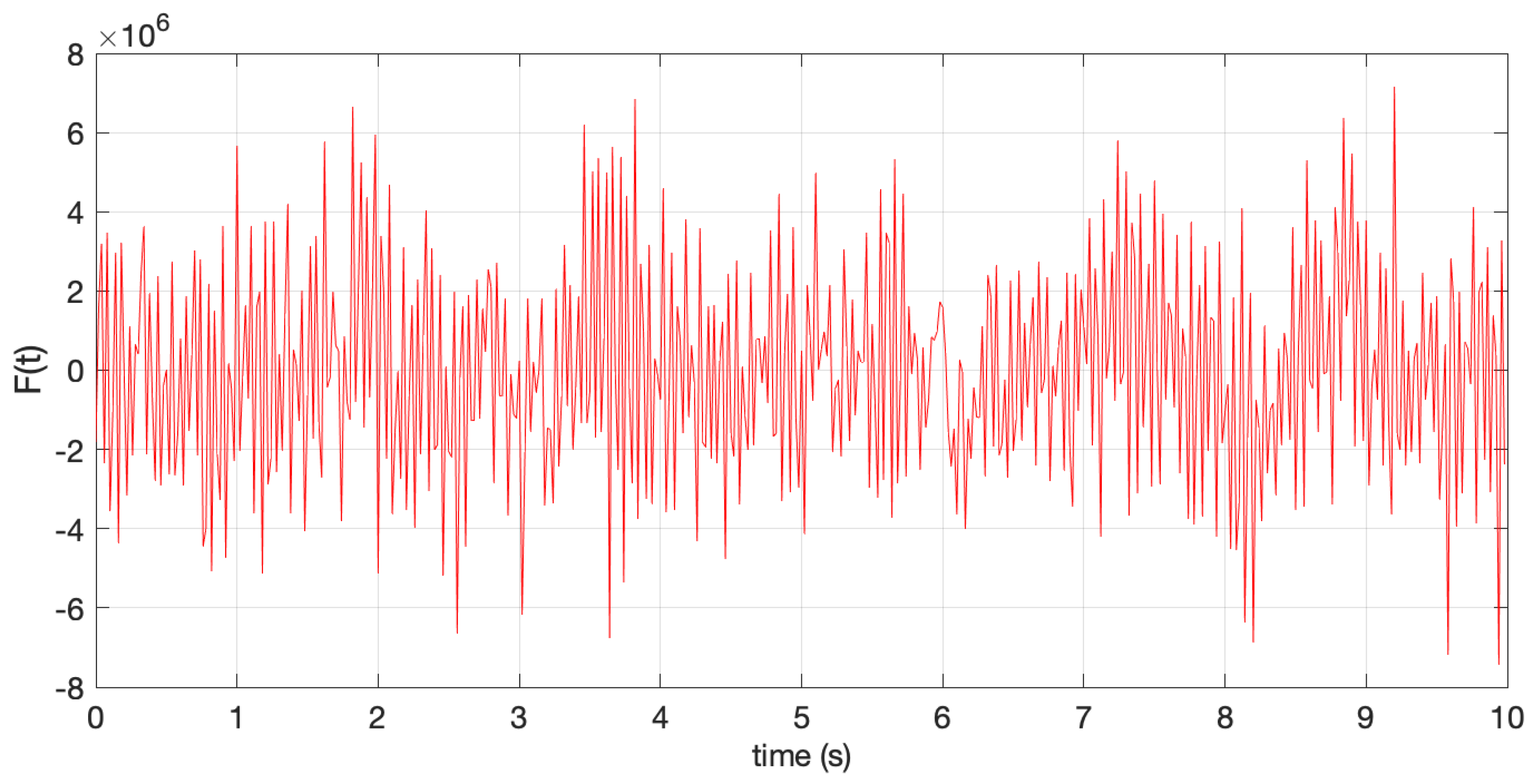
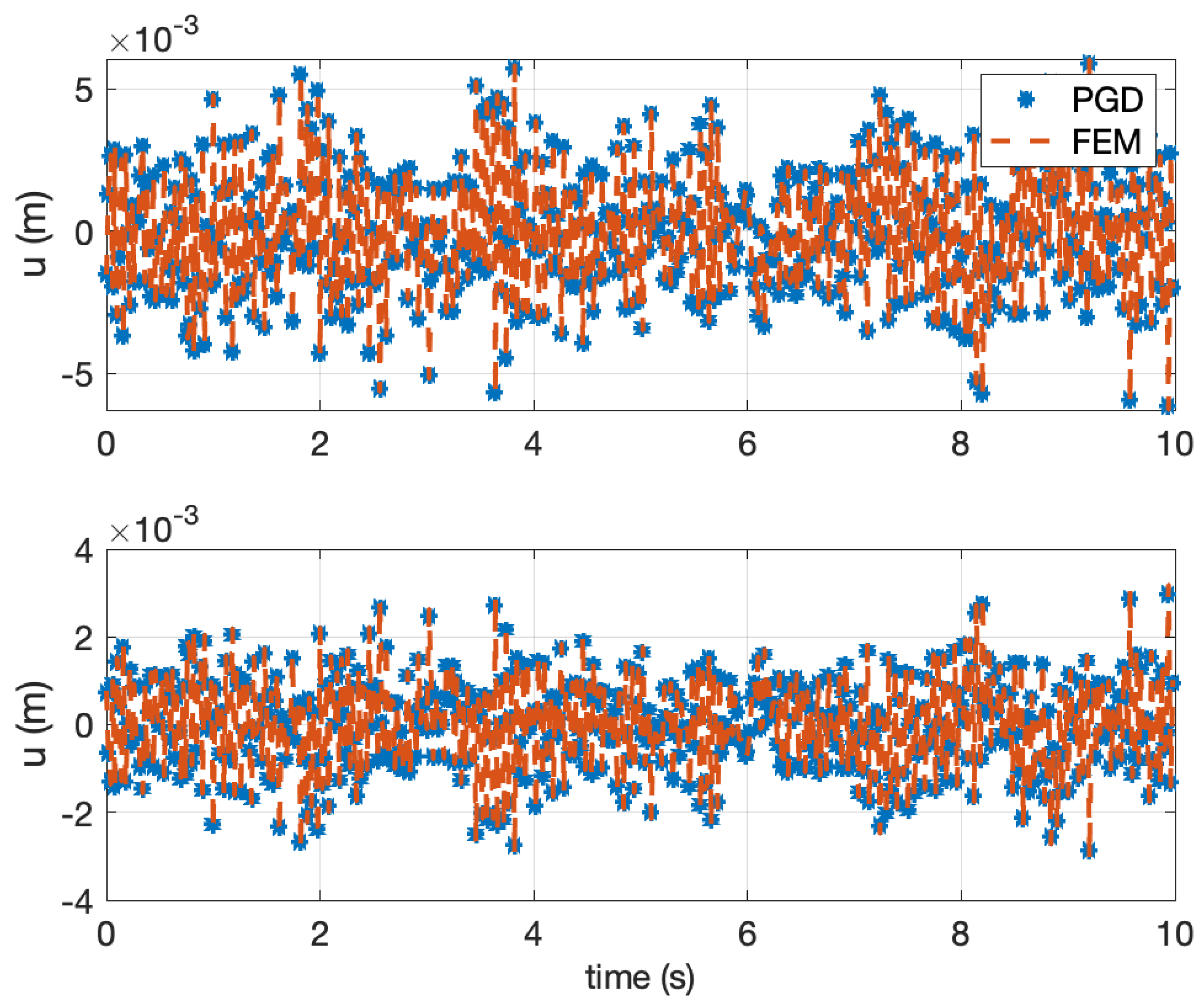
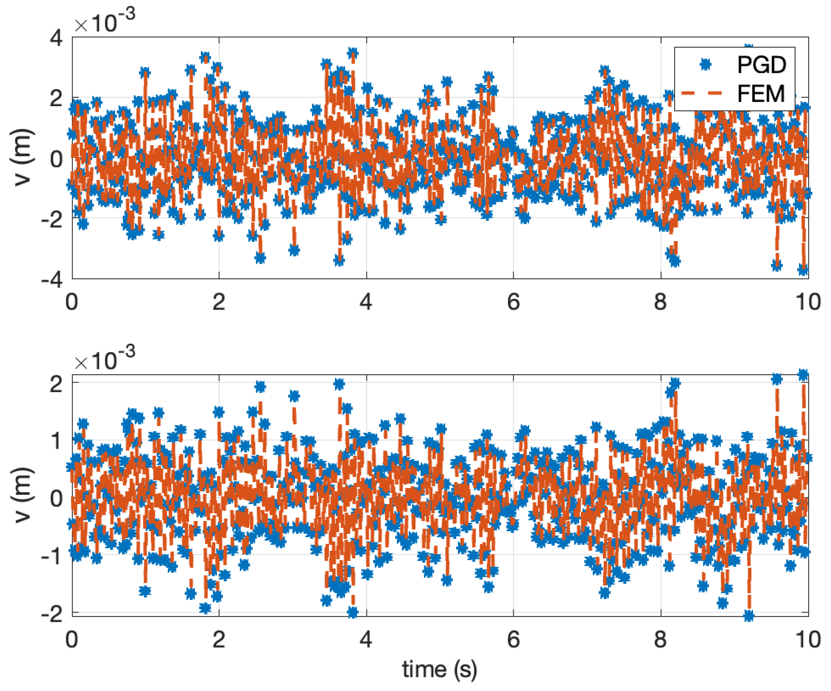
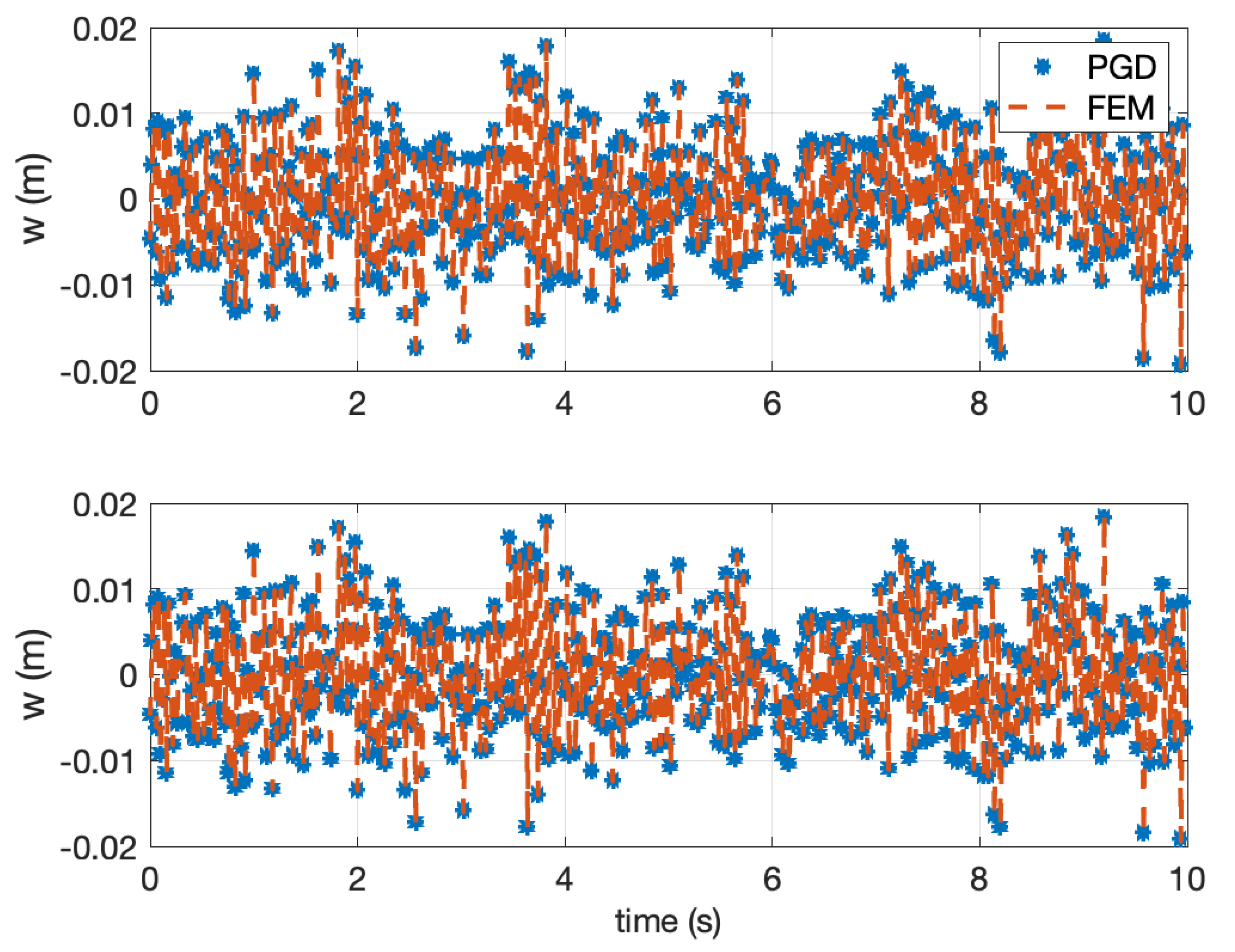
Now it is considered, for ${\mu }_1=2\times {10}^9$ Pa and ${\mu }_2=5\times {10}^8$ Pa, the more complex loading shown in Figure 5 that involves many frequencies. Figure 6 shows the x-component of the displacement at the top of both layers, whereas Figure 7 and Figure 8 show the other displacement components. Again, the particularized solution (PGD-based) and the reference one (FEM) agree in minute despite the loading complexity and its much richer spectral content, with the former evaluated instantaneously (real-time) whereas the latter, the reference one (FEM), is much more computationally expensive.

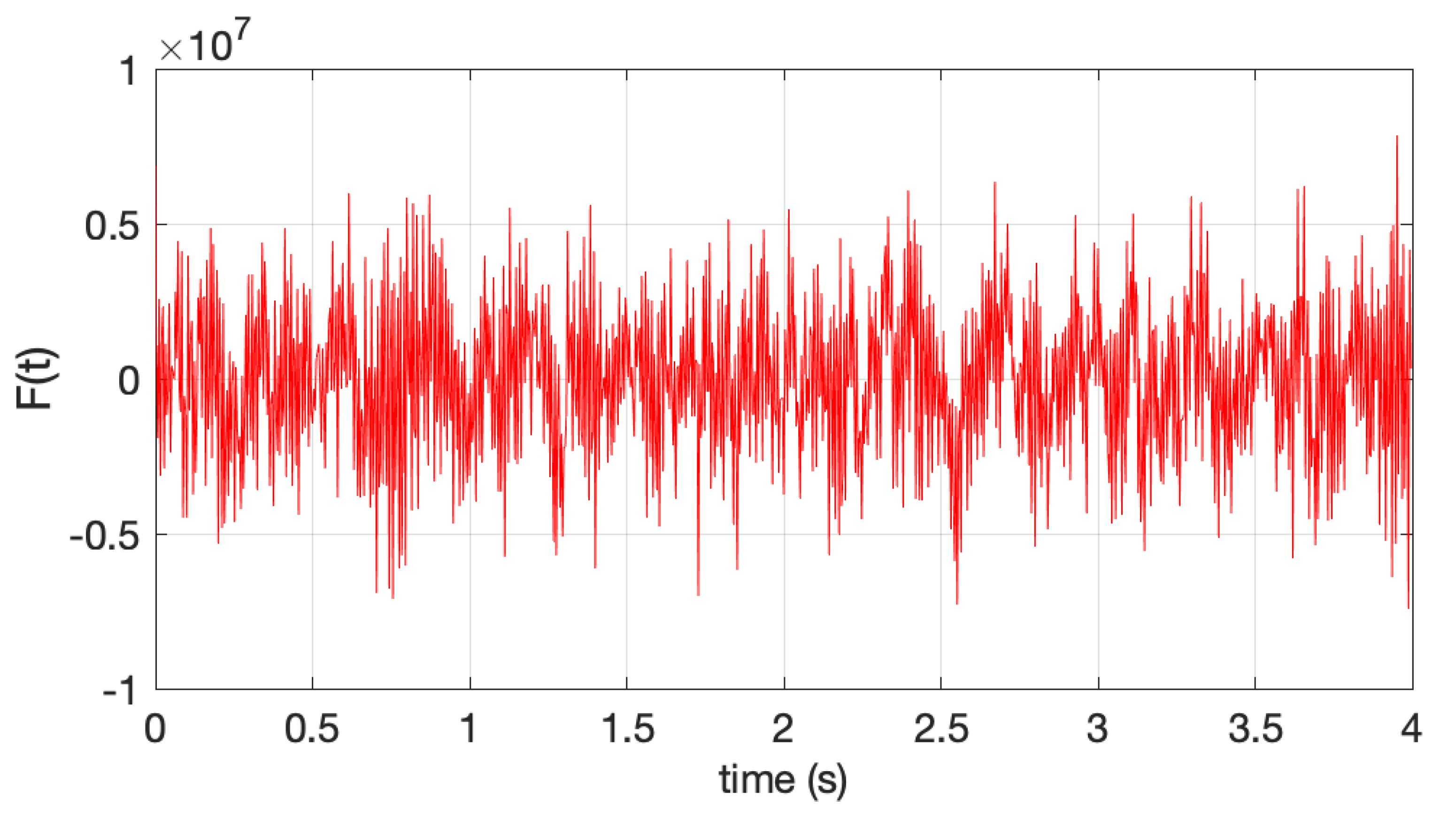
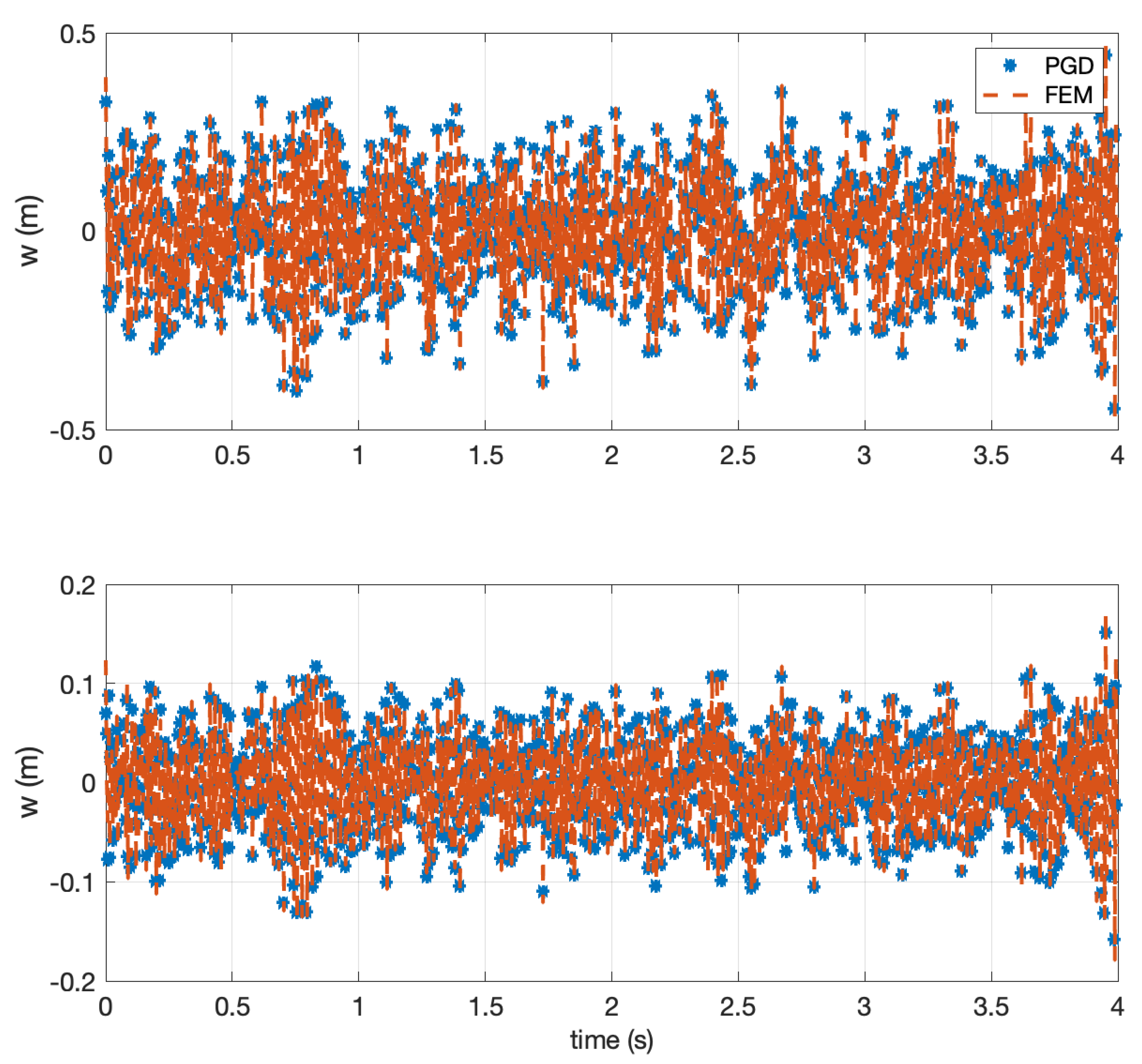
Finally, a larger frequency domain was considered ${\Omega }_{\omega }=2\pi (0,125)$s${}^{-1}$ in order to include natural frequencies inside, activated by the loading reported in Figure 9. For the same parameters that were considered previously, Figure 10 compares the z-component of the displacement at the center of the in-plane domain and at the top of both layers when using the PGD and the FEM, the latter computed by using the well experienced Newmark time integrator [14]. The solutions obtained by using both methods are again in prefect agreement.

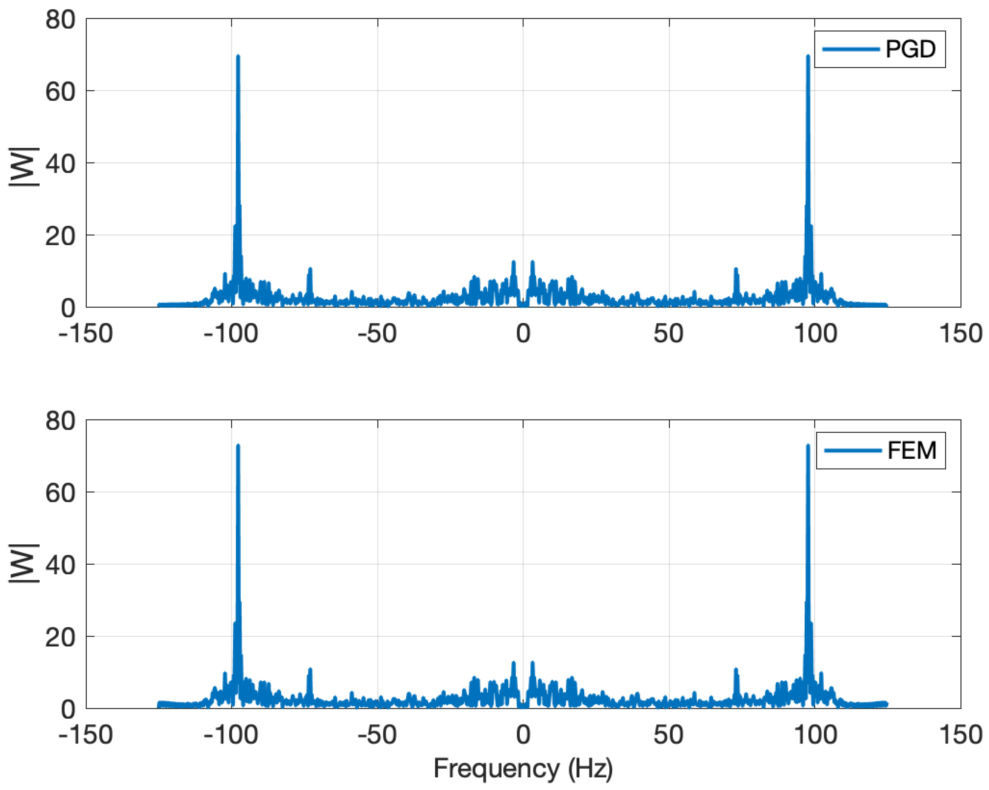
Finally, Figure 11 depicts the displacement amplitude versus the frequency, where the expected pics at the natural frequencies are noticed. Again, the solution computed by using the PGD is in perfect agreement with the one obtained by using the FEM, which is considered a reference solution.

As it can be noticed, the accuracy of the parametric solution particularization with respect to the reference solution is excellent, allowing evaluating in real-time (instantaneously) for any value of the parameters describing the soil behavior, helping engineers to improve design resilience.

5. Conclusions

The present work succeeded to extend the non-intrusive in-plane-out-of-plane separated representation to parametric dynamics. The procedure considers a non-intrusive formulation in order to overcome the difficulty related with the standard PGD algorithm when performing the in-plane-out-of-plane separated representation and, moreover, including parameters as extra coordinates. The results are very satisfactory when compared with a 3D FEM model, with the added value of its parametric nature.

Combining dimensionality reduction, that is, solving 3D problems at 2D cost, while incorporating parameters as extra-coordinates, and among them the frequency, the latter enabling the response evaluation instantaneously for any loading, and the whole performed in a non-intrusive manner, represents the main contribution of the preset work, never addressed until now, opening numerous possibilities in risk assessment as well as for improving structural designs.

References

- Chinesta, F.; Keunings, R.; Leygue, A. The Proper Generalized Decomposition for Advanced Numerical Simulations; A Primer, Springerbriefs; Springer: Berlin/Heidelberg, Germany, 2014. [Google Scholar]
- Chinesta, F.; Leygue, A.; Bordeu, F.; Aguado, J.V.; Cueto, E.; Gonzalez, D.; Alfaro, I.; Huerta, A. Parametric PGD based computational vademecum for efficient design, optimization and control. Arch. Comput. Methods Eng. 2013, 20, 31–59. [Google Scholar] [CrossRef]
- Bognet, B.; Leygue, A.; Chinesta, F.; Poitou, A.; Bordeu, F. Advanced simulation of models defined in plate geometries: 3D solutions with 2D computational complexity. Comput. Methods Appl. Mech. Eng. 2012, 201, 1–12. [Google Scholar] [CrossRef] [Green Version]
- Bognet, B.; Leygue, A.; Chinesta, F. Separated representations of 3D elastic solutions in shell geometries. Adv. Model. Simul. Eng. Sci. 2014, 1, 4. [Google Scholar] [CrossRef] [Green Version]
- Chinesta, F.; Leygue, A.; Beringhier, M.; Nguyen, L.T.; Grandidier, J.C.; Schrefler, B.; Pesavento, F. Towards a framework for non-linear thermal models in shell domains. Int. J. Numer. Methods Heat Fluid Flow 2013, 23, 55–73. [Google Scholar] [CrossRef] [Green Version]
- Vidal, P.; Gallimard, L.; Polit, O. Proper generalized decomposition and layer-wise approach for the modeling of composite plate structures. Int. J. Solids Struct. 2013, 50, 2239–2250. [Google Scholar] [CrossRef]
- Vidal, P.; Gallimard, L.; Polit, O. Shell finite element based on the proper generalized decomposition for the modeling of cylindrical composite structures. Comput. Struct. 2014, 132, 1–11. [Google Scholar] [CrossRef] [Green Version]
- Bordeu, F.; Ghnatios, C.; Boulze, D.; Carles, B.; Sireude, D.; Leygue, A.; Chinesta, F. Parametric 3D elastic solutions of beams involved in frame structures. Adv. Aircr. Spacecr. Sci. 2015, 2, 233–248. [Google Scholar] [CrossRef]
- Dumon, A.; Allery, C.; Ammar, A. Proper general decomposition (PGD) for the resolution of Navier-Stokes equations. J. Comput. Phys. 2011, 230, 1387–1407. [Google Scholar] [CrossRef] [Green Version]
- Dumon, A.; Allery, C.; Ammar, A. Simulation of heat and mass transport in a square lid-driven cavity with proper generalized decomposition. Numer. Heat Transf. Part B Fundam. 2013, 63, 18–43. [Google Scholar] [CrossRef] [Green Version]
- Ghnatios, C.H.; Chinesta, F.; Binetruy, C. 3D Modeling of squeeze flows occurring in composite laminates. Int. J. Mater. Form. 2015, 8, 73–83. [Google Scholar] [CrossRef]
- Leon, A.; De Luca, S.; Leygue, A.; Duval, J.L.; Chinesta, F. Non-intrusive proper generalized decomposition involving space and parameters: Application to the mechanical modeling of 3D woven fabrics. Adv. Model. Simul. Eng. Sci. 2019, 6, 13. [Google Scholar] [CrossRef] [Green Version]
- Clough, R.W.; Penzien, J. Dynamics of Structures; Civil Engineering Series McGraw-Hill: New York, NY, USA, 1993. [Google Scholar]
- Newmark, N.M. A method of computation for structural dynamics. J. Eng. Mech. Div. 1959, 85, 67–94. [Google Scholar]
- Bathe, J. Conserving energy and momentum in nonlinear dynamics: A simple implicit time integration scheme. Comput. Struct. 2007, 85, 437–445. [Google Scholar] [CrossRef]
- Boucinha, L.; Gravouil, A.; Ammar, A. Space-time proper generalized decompositions for the resolution of transient elastodynamic models. Comput. Methods Appl. Mech. Eng. 2013, 255, 67–88. [Google Scholar] [CrossRef] [Green Version]
- Ladeveze, P. The large time increment method for the analyze of structures with nonlinear constitutive relation described by internal variables. CR Acad. Sci. Paris 1989, 309, 1095–1099. [Google Scholar]
- Ladeveze, P.; Arnaud, L.; Rouch, P.; Blanze, C. The variational theory of complex rays for the calculation of medium-frequency vibrations. Eng. Comput. 1999, 18, 193–214. [Google Scholar] [CrossRef] [Green Version]
- Quaranta, G.; Argerich, C.; Ibanez, R.; Duval, J.L.; Cueto, E.; Chinesta, F. From linear to nonlinear PGD-based parametric structural dynamics. Comptes Rendus Mécanique 2019, 347, 445–454. [Google Scholar] [CrossRef]
Figure 1.
Case study: (a) In-plane view; (b) cross-sectional view.
Figure 2.
Harmonic loading.
Figure 3.
Displacement field (u, v, w) versus time at the mid-depth of the top layer (top) and bottom layer (bottom). As this figure aims to compare finite element method (FEM) and Proper Generalized Decomposition (PGD) solutions, due to the significant differences of the displacement values, for the sake of clarity, different scales are considered in each figure.
Figure 4.
Maximum strain at the top of the top layer. Because of the significant differences in the strain values, for the sake of clarity, different scales are considered in each figure.
Figure 5.
Loading involving a wider frequency content.
Figure 6.
x-component of the displacement at the top of both layers: (top) top layer and (bottom) bottom layer.
Figure 7.
y-component of the displacement at the top of both layers: (top) top layer and (bottom) bottom layer.
Figure 8.
z-component of the displacement at the top of both layers: (top) top layer and (bottom) bottom layer.
Figure 9.
Loading involving a larger frequency content.
Figure 10.
Figure 11.
Displacement amplitude W versus frequency at top of the top layer.
© 2020 by the authors. Licensee MDPI, Basel, Switzerland. This article is an open access article distributed under the terms and conditions of the Creative Commons Attribution (CC BY) license (http://creativecommons.org/licenses/by/4.0/).
Share and Cite
MDPI and ACS Style
Germoso, C.; Quaranta, G.; Duval, J.L.; Chinesta, F. Non-Intrusive In-Plane-Out-of-Plane Separated Representation in 3D Parametric Elastodynamics. Computation 2020, 8, 78. https://0-doi-org.brum.beds.ac.uk/10.3390/computation8030078
AMA Style
Germoso C, Quaranta G, Duval JL, Chinesta F. Non-Intrusive In-Plane-Out-of-Plane Separated Representation in 3D Parametric Elastodynamics. Computation. 2020; 8(3):78. https://0-doi-org.brum.beds.ac.uk/10.3390/computation8030078
Chicago/Turabian StyleGermoso, Claudia, Giacomo Quaranta, Jean Louis Duval, and Francisco Chinesta. 2020. "Non-Intrusive In-Plane-Out-of-Plane Separated Representation in 3D Parametric Elastodynamics" Computation 8, no. 3: 78. https://0-doi-org.brum.beds.ac.uk/10.3390/computation8030078
Note that from the first issue of 2016, this journal uses article numbers instead of page numbers. See further details here.