Graph Reachability on Parallel Many-Core Architectures


Department of Control and Computer Engineering, Politecnico di Torino, Corso Duca degli Abruzzi 24, I-10129 Turin, Italy
*
Author to whom correspondence should be addressed.
Computation 2020, 8(4), 103; https://0-doi-org.brum.beds.ac.uk/10.3390/computation8040103
Submission received: 19 October 2020
/
Revised: 20 November 2020
/
Accepted: 26 November 2020
/
Published: 2 December 2020
Abstract
:Many modern applications are modeled using graphs of some kind. Given a graph, reachability, that is, discovering whether there is a path between two given nodes, is a fundamental problem as well as one of the most important steps of many other algorithms. The rapid accumulation of very large graphs (up to tens of millions of vertices and edges) from a diversity of disciplines demand efficient and scalable solutions to the reachability problem. General-purpose computing has been successfully used on Graphics Processing Units (GPUs) to parallelize algorithms that present a high degree of regularity. In this paper, we extend the applicability of GPU processing to graph-based manipulation, by re-designing a simple but efficient state-of-the-art graph-labeling method, namely the GRAIL (Graph Reachability Indexing via RAndomized Interval) algorithm, to many-core CUDA-based GPUs. This algorithm firstly generates a label for each vertex of the graph, then it exploits these labels to answer reachability queries. Unfortunately, the original algorithm executes a sequence of depth-first visits which are intrinsically recursive and cannot be efficiently implemented on parallel systems. For that reason, we design an alternative approach in which a sequence of breadth-first visits substitute the original depth-first traversal to generate the labeling, and in which a high number of concurrent visits is exploited during query evaluation. The paper describes our strategy to re-design these steps, the difficulties we encountered to implement them, and the solutions adopted to overcome the main inefficiencies. To prove the validity of our approach, we compare (in terms of time and memory requirements) our GPU-based approach with the original sequential CPU-based tool. Finally, we report some hints on how to conduct further research in the area.
1. Introduction
The rapid accumulation of huge graphs from a diversity of disciplines, such as geographical navigation, social and biological networks, XML indexing, Internet routing, and databases, among others, requires fast and scalable graph algorithms. In these fields data are normally organized into a directed graph (or digraph) and the ancestor-descendant relationship of nodes is often required. Thus, given a directed graph finding whether there is a simple path leading from a vertex v to another vertex u is known as the reachability problem [1,2,3,4,5,6,7,8,9]. Reachability plays an important role in several modern algorithms since it is the underlying steps of many other applications.
State-of-the-art methodologies to solve the reachability problem are based either on algorithms visiting the graph or on computing its Transitive Closure. Unfortunately, traversal algorithms, such as breadth-first (BFS) and depth-first (DFS) searches, have linear time complexity (in the graph size) for each query. Moreover, the materialization of the whole transitive closure is very space-consuming as it implies a quadratic memory occupation (in the graph size). As a consequence, these strategies do not scale well for large graphs (e.g., beyond few millions of vertices and edges), and most practical reachability algorithms trade-off their characteristics and ends-up lying somewhere in between them. In the so-called graph labeling methods, the vertices are assigned labels such that the reachability between nodes can be decided using these labels. Current approaches belonging to this category include two phases. During a pre-processing step, they create the “index”, trying to minimize the amount of information added to each node of the graph. During the exploitation phase, they use the index to speed-up the query resolution time. Selecting the correct trade-off between the indexing space and the querying time often represents the main attribute characterizing an algorithm. The biggest limitation of state-of-the-art algorithms using this approach lies in their ability to efficiently process large graphs. Then, scalability has become one of the most significant metrics to compare reachability approaches.
Interestingly, general-purpose computing on GPUs is increasingly used to deal with computationally intensive algorithms coming from several domains [10,11,12]. The advent of languages such as OpenCL and CUDA have transformed general purpose GPU (Graphical Processing Unit) into highly-parallel systems with significant computational power. Many-core parallel systems have been proved to scale gracefully by exploiting their rapidly improving hardware features and their increasing number of processors. As a consequence, since 2006, when the first version of CUDA was released, there has been a continuous effort to redesign algorithms to exploit the large degree of data parallelism, the ever-increasing number of processors, and the huge bandwidth available on GPUs. More specifically, GPUs are designed to execute efficiently the same program concurrently over different data. For that reason, recently there has been an increasing focus to produce software processing graph in CUDA, both from NVIDIA, with its NVIDIA Graph Analytic library, and from independent projects, such as the recent Gunrock library [13].
In this context, as sequential programming has often become “parallel programming” [14,15], we present a multi-core CPU-based and a many-core GPU-based design of the reachability strategy called GRAIL [16]. GRAIL (Graph Reachability Indexing via RAndomized Interval Labeling) was designed to be conceptually simple, efficient, and scalable on large graphs. The algorithm presents linear time complexity and linear memory requirements, and, after a pre-processing phase, it is able to solve reachability queries with a cost varying from constant to linear in the graph size in terms of computation time. In this work, our target is to re-design the original algorithm to make it exploitable on computation devices allowing a high degree of data parallelism, such as the so called SIMT (Single Instruction, Multiple Threads) systems. The main difficulty to implement this transformation is due to the fact that GRAIL executes a series of DFSs to generate all the nodes’ label during the labeling phase and to exploit them during the query phase. DFS is an intrinsically recursive procedure, as it recursively visits each path in-depth before moving to the next path. This logic generates two orders of problems. Firstly, in-depth visits are very difficult to parallelize. Secondly, even when using Dynamic Parallelism, GPUs do not allow more than 24 in-depth recursion levels. In turn, this limitation would restrict applicability to very small graphs only. For the above reasons, the first step required to re-design the original algorithm to the target hardware device, is to modify its logic flow to increase the number of operation performed in parallel and to formally remove recursion. Notice that, explicitly substituting recursion by implementing a “user” stack would be inefficient both in terms of time and of memory requirements. Adopting one (or more) “user” stack(s) (possibly one for each thread) would imply using an unpredictable quantity of memory to sustain the work of each thread with eventually high contention problems. As a consequence, following Naumov et al. [17,18], we exploit some property of Direct Acyclic Graphs (DAGs) to label them adopting a non-recursive procedure. We substitute one single depth-first visit finding a label pair for each node, with a sequence of four breadth-first traversals. The first three BFSs will be used to label nodes with their post-order outer rank. The last one will be used to complete each label, computing the in-order rank starting from the previously computed post-order label. In any case, a BFS iteratively expand the “frontier” set of states, thus it enables a much higher degree of data parallelism and it is intrinsically non-recursive. Obviously, as our algorithm will finally perform four breadth-first traversals of the graph instead of one single depth-first visit, it will be essential to efficiently implement BFSs on GPUs. As a consequence, following other recent researchers in the area [13,19,20,21], we will dedicate part of our work to describe how to adapt state-of-the-art BFSs to general purpose GPU computing. Our data analysis, on large standard benchmarks and home-made graphs, will prove that our GPU-based implementation is quite competitive with the original CPU-based reachability tool and it presents interesting speed-up factor in many cases. Our results also further motivate new research paths, analyzing those cases in which heterogeneous computational units may work together to solve more efficiently huge and complex tasks where reachability may just be a part of a wider scenario.
As far as the implementation language is concerned, nowadays, CUDA and OpenCL are the leading GPGPU frameworks and each one brings its own advantages and disadvantages. Even if OpenCL is supported in more applications than CUDA, the general consensus is that CUDA generates better performance results [22,23,24] as NVIDIA provides extremely good integration.
For that reason, we provide an implementation of the proposed solution developed on CUDA-based systems, even if an OpenCL implementation would imply moderate modifications and corrections.
It has to be noticed that this paper is an extended version of the conference paper in Reference [25]. The current paper extends the original one in several directions. First of all, it completely revises the original notation and it presents the pseudo-code of all adopted functions. Secondly, it enriches the original work with an analysis of the final algorithm in terms of time and memory complexity. Finally, it reformulates all experimental results, now including not only the largest standard benchmarks but also large home-made graphs. As far as we know, some of the previous contributions are presented for the first time.
Roadmap
The paper is organized as follow. Section 2 introduces the related works on graph reachability, the notation adopted, and the necessary background on graph labeling and SIMT architectures. Section 3 briefly describes a multi-core CPU-based implementation, while Section 4 introduces the GPU-based strategy to perform labeling. After that, Section 5 concentrates on how to solve reachability queries on GPU-based systems. Section 6 discusses our experimental data analysis. Section 7 concludes the paper summarizing our work and reporting some comments on possible future works.
2. Background
2.1. Related Works
The graph reachability problem has been extensively studied over the years. A first main block of works concentrate on the classical problem, that is, it focuses on static and directed acyclic graph on which the main target is to improve the efficiency to solve reachability queries. These works can be divided into three main categories.
The first category [16,26,27] includes on-line searches. These approaches proceed in two phases. During the first one, instead of fully computing the transitive closure of the graph, they create auxiliary labeling information for each vertex. During the second one, they use this information to reduce the query time by pruning the search space. Among the advantages of these approaches it is worth mentioning their applicability to very large graphs. Unfortunately, in many cases the query phase is from one to two orders of magnitude slower than the one obtained with methods belonging to the other two categories.
The second category [3,28] includes the so-called reachability oracle methods, more commonly known as hop labeling strategies. The core idea is the following one. Each vertex v of the graph G is labeled with two sets. The first set includes all vertices reachable from v, that is, . The second set contains all vertices that can reach v, that is, . Once and are known for all nodes, a query to check whether v reaches u can be solved by verifying if there is at least a common hop between and , that is, . This strategy somehow lie in between the other two categories. For that reason, it should be able to deliver indices more compact than the third category and offer query times smaller than the first class of approaches.
The third category [1,29,30,31,32,33] includes all approaches trying to compute a condensed form of the transitive closure of the graph. To compress the transitive closure, these method store for each vertex v in the graph G a compact representation of all vertices reachable from v, that is, . Once this is done, the reachability from vertex v to u can be checked by verifying whether vertex u belong to the set . Obviously, the experimental evidence show how these approaches are the fastest in terms of query efficiency. Unfortunately, representing the transitive closure, even if in a compressed format, may still be very expensive. For that reason, these approaches do not scale well enough to be applicable on large graphs.
Some more recent works also study the same problem under a different perspective or problems related to the original one. Zhu et al. [4] concentrate on the application of existing techniques on dynamically changing graphs commonly encountered in practice. The authors adopt a reachability index able to handle vertex insertions and deletions, and they show that their updated algorithm can be used to improve existing techniques on static graphs. Su et al. [5] exploit k-min-wise independent permutations to smartly process reachability queries. They propose a new Bloom filter labeling scheme that can be proved to have bounded probability to answer reachability queries and a high power to answer more reachability queries directly. Strzheletska et al. [6] focus on processing spatio-temporal reachability queries for large disk-resident trajectory data-sets. In this application, information cannot be instantaneously transferred from one object to another, thus forcing interacting objects to stay in contact for some time interval and making the query processing even more challenging. Mäkinen at al. [7] concentrate on the minimum path cover problem, that is, on finding a minimum-cardinality set of paths that cover all the nodes of a directed acyclic graph. More specifically, the authors study the case of DAGs with a small width, and they introduce a general framework to extend sparse dynamic programming to DAGs. Peng et al. [8] analyze the problem of label-constrained reachability query which is more challenging than the standard problem because the number of possible label constraint sets is exponential in the size of the labels. The authors propose a label-constrained 2-hop indexing technique with novel pruning rules and order optimization strategies. Pacaci et al [9] study persistent query evaluation over streaming graphs and they focus on navigational queries that satisfy user-specified constraints. The authors propose deterministic algorithms to uniformly evaluate persistent Regular Path Query under both arbitrary and simple path semantics.
2.2. Notation
In the sequel, we will refer to directed graph as , where V is the set of vertices and E the set of directed edges. We will also refer to the cardinality of V and E with n and m, respectively. In our implementations, we will store a graph G adopting the so called Compressed Sparse Row (CSR) representation. CSR is particularly efficient when large graphs must be represented, since it is basically a matrix-based representation that stores only non-zero elements of every row. Using this strategy, we are then able to offer a fast access to the information related to each row, avoiding useless overhead for very sparse matrices at the same time. Essentially, in the CSR format edges are represented as a concatenation of all adjacency lists of every node. Two additional arrays are used to store information about the cardinality of each adjacency list and to index the adjacency list of each vertex in the main array. Figure 1b reports the CSR representation for the graph of Figure 1a. As an example, in order to iterate through the children of node 3, we would have to access the 2 elements of the adjacency list array starting from the node at position 4, since the cardinality of node 3 is 2 and the first children is in position 4. We also point out that, traditionally, the array storing the cardinalities is not necessary, since these cardinalities can be computed through two accesses to the array storing the indices. Unfortunately, GPU architectures set a high price for sequential accesses on consecutive array elements by the same thread. Thus, in our application, it is preferable to retrieve the cardinality using one extra array.
To check whether there is a path that goes from vertex v to node u, we use the notation which indicate the standard reachability query. Moreover, we write to indicate that such a path exists, and if it does not exist.
We also suppose each vertex v has a set of attributes associated with it. These attributes will store for each node any information our algorithms need. For example, we will indicate with the interval label associated with vertex v, with the path leading from the root of the directed tree to vertex v, with and the set of parents and children of node v, and so forth.
As a final comment, please recall that reachability on directed graphs can be reduced to reachability on Directed Acyclic Graphs (DAGs). In fact, for every directed graph it is possible to find all strongly connected components (SCCs) with a liner cost and to build an equivalent but more compact graph. Once this step is done, the reachability query on a directed graph can be answered by checking whether in the condensation graph the SSC of v and the SCC of u, namely and , coincide or whether . Henceforth, we assume that all our graphs are directed and acyclic.
2.3. GPUs and CUDA
GPGPU (General Purpose GPU) is the use of a GPU (Graphics Processing Unit), which would typically only manage computer graphics, to execute tasks that are traditionally run by the CPU. GPGPUs enable data transfer in a bi-directional way, that is, from the CPU to GPU and from the GPU to CPU, such that they can hugely improve efficiency in a wide variety of tasks. OpenCL and CUDA are software frameworks that allow GPU to accelerate processing in applications where they are respectively supported. OpenCL is the leading open source framework. CUDA, on the other hand, is the leading proprietary framework. The general consensus is that if an application supports both CUDA and OpenCL, CUDA will be faster [22,23,24] as the integration is always extremely good and well supported. For that reason, we describe the corrections required to the multi-core CPU-based algorithm to handle the heavy workload unbalance and the massive data dependency of the original recursive algorithm on the CUDA framework.
In a NVIDIA architecture, parallelization is obtained by running tasks on a large number of streaming processors or CUDA cores. CUDA cores can be used to run instructions, such that all cores in a streaming multiprocessor execute the same instruction at the same time. This computational architecture, called SIMT (Single Instruction, Multiple Threads), can be considered as an advanced form of the SIMD (Single instruction, Multiple Data) paradigm. The code is normally executed by groups of 32 threads. Each group is called “warp”. Memory access schemes can also strongly influence the final application performance. GPUs support dynamic random access memory, with an L2 cache with low-latency, and an L1 cache with a high-bandwidth per streaming multiprocessor.
CUDA allows programmers to exploit the different parallel architecture of graphic processing units for certain categories of programs that require massive computing power. Graphics computing usually involves large matrices modeling pixels on the screen, on which lots of heavy mathematical calculations have to be quickly computed in order to create new images that have to be shown on the screen with fast refresh rates. This mechanism offer offers high level of data-parallelism, because such mathematical operations can be done independently in parallel on each pixel.
2.4. The GRAIL Approach
When taking about graphs, interval labeling consists in assigning to each node a label representing an interval. Intervals can be generated using different strategies. The most common ones are the pre-post and the min-post scheme. GRAIL [16] uses the latter approach. This approach assigns to each graph node a label made-up of two values, that is, , forming a closed interval. Let us suppose we deal with a Direct Tree (DT) in which every node v has a single parent. In our notation, we indicate with:
- the rank of vertex v in a post-order traversal of the graph G. is also referred to as the “outer rank” of v. Outer ranks can be computed visiting the DT recursively from the roots to the leaves such that all children of a node are visited adopting a pre-defined and fixed order. In this way, each node is “discovered” moving “down” along the recursion process and it is “released” moving “up”. We initially assign 1 to . Then, we assign to a vertex every time the vertex is released during the visit and we increment after each assignment.
- is the starting value of each interval and it is also referred to as “inner rank” of v. The inner rank is computed starting from the outer rank as follow. If the vertex v is a leaf, than is equal to . If the vertex v is an internal node, is equal to the minimum value among all outer-ranks of the descendants of v, that is, .
This approach guarantees that the containment between intervals is equivalent to the reachability relationship between the nodes, since the post-order traversal enters a node before all of its descendants, and leaves after having visited all of its descendants.
Given two nodes v and u and their labels, and , GRAIL checks whether by verifying the interval containment of the two vertices, that is, , if and only if . For the DT of Figure 2a labels can be computed through a simple DFS, with a construction time which is linear in the number of vertices. We suppose that the DFS follows the left child of each node before moving along the right child. Then, these label intervals can be used to check the reachability between every couple of vertices. For example, , since , and , since .
Unfortunately this simple procedure is no longer valid for DAGs. In fact, if we move from a DT to a DAG, min-post labeling may be used to correctly detects all reachable pairs but it may also falsely detect as reachable pairs that are actually unreachable. For example, the DAG of Figure 2b derived from the DT of Figure 2a with the addition of a few edges (highlighted in bold). Unfortunately, node I has vertices E, G and H as parents and its inner rank will propagate to all of them. This entails that two nodes that do not reach each other but have a common descendant, such as E and F, can be easily marked as reachable. In fact, but .
One of the possible strategy to mitigate the above problem, the one adopted by GRAIL, is to compute multiple interval labels. As a consequence we can perform multiple randomized visits of the graph, create a label pair during each visit, and using multiple intervals for every vertex at the end of the process. We will use d to indicate the number of label pairs. An example of labeling with , that is, with two label pairs, is represented in Figure 2c. This time, we suppose that the second DFS follows the right child of each node before moving along the left child. In this case, we can see that we have label inclusion on the first label pair, that is, , but not on the second label pair, that is, , thus we may conclude that .
Usually, a small number of labels d is sufficient to drastically reduce the number of exceptions. For example, one can notice that the number of exceptions in the graph of Figure 2b decreases from 15 to just 3 by using two label pairs instead of one. Since the number of possible labelings is exponential, usual values for d are in the range , regardless of the size of the graph.
Unfortunately, even with multiple label pairs, unreachable nodes can still be detected as reachable. For that reason, once we have ruled-out all unreachable nodes, all remaining reachable pairs must be explicitly verified. Two different strategies are usually adopted. The first one, consists in creating an exception list for each vertex a priory. Unfortunately, as creating and storing exception lists may be extremely expensive, this strategy is rarely adopted. The second one is to resort to an extra depth-first search to rule-our false positive. In this case, the extra visit required for each positive pair is much faster than the original graph visit, as is may use interval comparison to prune the tree search at every level. Therefore, this will be the strategy used in our implementation.
3. Parallel Graph Exploration
Parallelizing the previous approach can be trivial, but results may be quite limited and disappointing. Algorithm 1 presents a first possible solution. Given the original graph G and the set of all queries S, it splits the process into the labeling (lines 1–3) and the query phase (lines 4–6), and it parallelizes both of them. As each single DFS is hardly parallelizable, during the labeling phase parallelization is limited to create each single labeling pair (within the set of d labeling pairs) on a different core. For the query phase, the parallelization may run all queries S diving them into subsets s of k queries, and solving each subset using a different thread.
| Algorithm 1 The labeling and the query phases: A trivial parallel approach. | |
| ParallelLabelingAndQuery (G, S) | |
| 1: | fori varying from 1 to d label pairs in parallel do |
| 2: | ComputeLabels (G, i) |
| 3: | end for |
| 4: | fors in the set S of all queries in parallel do |
| 5: | SolveQuery (G, s) |
| 6: | end for |
Unfortunately, even this trivial divide-and-conquer approach, with its limited degree of parallelism, cannot be easily extended to GPU computations. In spite of their enormous computational throughput, GPUs are particularly sensitive to several programming issues and breadth-first traversals represent a class of algorithms for which it is very hard to obtain a significant performance improvement from parallelization. As a matter of fact, GPUs are suppose to perform poorly on data structures such as graphs for several reasons. As access patterns to memory have a high correlation with the structure of the input graph, optimizing the memory requirements of a BFS is hard. Moreover, code parallelization introduces contention among threads, control flow divergence, load imbalance and memory inefficiency, parameters that together lead to an under-utilization of multi-threaded architectures. To mitigate the above issues, previous approaches performing parallel graph algorithms (for example, see Merrill et al. [34]) based their implementations on two key architectural GPU features. The first one is hiding memory latency by adopting multi-threading and overlapped computations. The second one is fine-grained synchronization by resorting to specific atomic read-write operations. In particular, atomicity is useful especially to coordinate the manipulation of dynamic shared data and to arbitrate contentions on shared objects. Unfortunately, even if modern GPU architectures provide these features, the serialization forced by atomic synchronization is particularly expensive for GPUs in terms of efficiency. Moreover, even atomic mutual exclusion does not scale well to thousands of threads. Furthermore, the occurrence of fine-grained and dynamic serialization within the SIMD width is much more expensive than between overlapped SMT threads. We will concentrate on our efforts to parallelize the labeling phase and the query phase on a GPU in the next two sections.
4. Our GPU-Based Labeling Strategy
DFS-based labeling approaches traverse a graph in-depth, adopting recursion, and following a pre-defined order of the nodes during the visit, given by the topology of the graph. Moreover, these algorithms usually update global variables storing inner and outer rank values. These variables need to be properly protected and accessed in mutual exclusion in parallel applications. These features are conspicuous limitations for parallelization, as already noted by Aggarwal et al. [35] and by Acar et al. [36], among the others. However, a graph can also be visited breadth-first, by exploring the current set (i.e., the frontier set) of vertices in-breadth. A BFS can proceed in parallel on all vertices of the frontier set, allowing a higher degree of data parallelism. Unfortunately, we do not just have to visit a graph, but we have to label all visited vertices, operation easily performed in-depth but much harder when processing node in breadth-first.
The key to compute label pairs while visiting the graph in breadth-first is based on the consideration that finding the post-order rank of a node in a directed tree is equivalent to computing an offset based on the number of nodes standing below and on the left of the node itself. Following a process first presented by Naumov et al. [17,18], we will substitute the original DFS-based labeling approach with a BFS-based one. The latter one, including three BFSs, will be able to compute the outer rank of each node, based on the previous observation, and it will be capable to proceed in parallel on every vertex each node can reach. Note that, even if this process can generate a complete label pair for each node, this labeling scheme, using separate counters for the pre and post-order ranks, will be unsuited for label inclusion. Thus, during the first three BFSs, we compute only the outer rank of each vertex v, and we adopt an extra breadth-first visit to recompute its inner rank and to build the entire min-post label for v, that is, . The resulting process, which includes four breadth-first visits, is illustrated by the running example of Figure 3 and described by Algorithm 2. We will analyze each main step in one of the following four subsections.
| Algorithm 2 The labeling computation phase based on four BFSs. | ||
| ComputeLabels (G) | ||
| 1: | DT = DAGtoDT (G) | // Step 1 |
| 2: | ComputeSubgraphSize (DT) | // Step 2 |
| 3: | ComputePostOrder (DT) | // Step 3 |
| 4: | ComputeMinPostLabeling (DT) | // Step 4 |
4.1. Step 1
The starting point of our running example is represented in Figure 3a. This is a very simple DAG G, including only 7 nodes, for the sake of simplicity. Figure 3b shows the DT obtained from the previous graph through the application of function DAGtoDT, called at line 1 of the high-level pseudo-code of Algorithm 2. To transform a DAG into a DT, function DAGtoDT may proceed in different way. The core idea is to select a parent for each vertex v of the original graph G and to erase all edges leading to v from all other parents. The so called “path based method” follows an intuitive approach. It essentially traverses the graph breadth-first, visiting the nodes top-down, and it assigns to each vertex the first encounter parent. In other words, a path to a vertex v is retained only when v has not been reached by a previous path. When two paths leading to a node are found, a node-by-node comparison of the two paths takes place. This comparison starts from the root and proceeds until a decision point is found and solved by selecting the path with the “smaller” node according to the ordering relationship in the graph.
The corresponding pseudo-code is shown in Algorithm 3. The function traverses the graph top-down, from roots to leaves and it stores the path used to reach each node from one of the roots in an array. As introduced in Section 2.2, we suppose such an array (named path) and other attributes (such as the parents, the children, etc.) are associated with each vertex v and references as , , and so forth. We also suppose to manipulate two queues (namely, and ) with standard functions (such as Init, Push, and Pop) properly protected by synchronization strategies. In reality, the actual implementation of these queues will be described in Section 4.5. Once initialized the path and the parent for all vertices, and the queue , function DAGtoDT considers, for all vertices in the first queue in parallel (line 6) all children in parallel (line 8). For each child, the function computes the new path to reach it (line 9). If the new path proceeds the current one (line 10), the latter is updated (line 11) and v is set as the proper parent of u. The comparison on line 10 can be performed by storing the path nodes in a linear array, aligning the arrays on the left and comparing the elements pairwise left-to-right until a mismatch is found. More details on how this phase can be optimized, can be found in References [17,18]. For example, the memory required to store paths can be reduced from to . This can be done by storing paths in chained linked list of blocks of size k. If the path completely fits into a block, then we store it there. Otherwise, if it does not fit, we store only the tail of the path in the block and we point to its “parent” block. By chaining the blocks in this way, it is also possible to reuse the path already stored for earlier nodes, therefore saving memory. The comparisons can be performed in parallel. A further possible optimization is related to path pruning. In a graph nodes with a single outgoing edge will never be a decision point. As a consequence, nodes with only a single outgoing edge do not affect the path comparison and do not have to be included in any path. A last possible optimization derives from path compression. As the number of outgoing edges is always significantly smaller than the total number of nodes, it is possible to associate a lexicographic order to each edge and to use this value to specify paths. While storing a node typically requires 32 (or 64) bits, if there are at most o outgoing edges from a node, the compression rate is (or ).
4.2. Step 2
Figure 3c reports the same directed tree of Figure 3b in which each vertex v is associated with , that is, the size of the subgraph rooted at v. The pseudo-code to compute is represented by Algorithm 4, which implements the second step within by the high-level procedure of Algorithm 2.
| Algorithm 3 Step 1: From DAG to DT with a top-down BFS. | |
| DAGtoDT (G) | |
| 1: | for each vertex v in parallel do |
| 2: | = = |
| 3: | end for |
| 4: | Init (, ) |
| 5: | while (≠) do |
| 6: | for each vertex v∈ in parallel do |
| 7: | Init (, ∅) |
| 8: | for each vertex u∈ in parallel do |
| 9: | = + v |
| 10: | if ( ≤ ) then |
| 11: | = |
| 12: | = v |
| 13: | end if |
| 14: | Set as visited |
| 15: | if (all incoming edges of u are visited) then |
| 16: | Push (, u) |
| 17: | end if |
| 18: | end for |
| 19: | end for |
| 20: | = |
| 21: | end while |
| Algorithm 4 Step 2: Subgraph size computation with a bottom-up BFS. | |
| ComputeSubgraphSize (DT) | |
| 1: | Init (, ∅) |
| 2: | for each vertex v in parallel do |
| 3: | = 0 |
| 4: | if (v is a leaf) then |
| 5: | Push (, v) |
| 6: | end if |
| 7: | end for |
| 8: | while (≠) do |
| 9: | for each vertex v∈ in parallel do |
| 10: | Init (, ∅) |
| 11: | for each vertex u∈ in parallel do |
| 12: | Set edge as visited |
| 13: | if (each outgoing edge of u is visited) then |
| 14: | Push (, u) |
| 15: | end if |
| 16: | end for |
| 17: | end for |
| 18: | for each vertex v∈ in parallel do |
| 19: | = prefix sum on |
| 20: | end for |
| 21: | |
| 22: | end while |
Function ComputeSubgraphSize essentially traverses the graph adopting a bottom-up BFS. During the visit, every time a vertex v is encountered, the size of the subgraph rooted at v is propagated upward to its parent u. More in details, the algorithm works as follow. All subgraphs sizes are initialized to zero (line 3), and all leaves are inserted into a first queue (line 5). During the outer iterative construct (line 9), the algorithm proceeds in parallel by extracting nodes from and by visiting their parents in the inner cycle (line 11). During each iteration of the inner cycle, the edge , where u is the parent and v is the child, is visited (line 12) and used to propagate upward. When a parent vertex u has been visited by all of its children, it is inserted on the second queue . This queue stores all the vertices that will be visited during the next outer iteration. The desired subgraph size , for each node v, can finally be computed operating a prefix-sum (The prefix sum, or cumulative sum, of a sequence of numbers is a second sequence of numbers such that each is the sums of prefixes, that is, , , , etc.) on the size of all the children of v (line 19). As a last observation please note that the algorithm proceeds bottom-up, and this implies that it is necessary to wait until a parent has been visited by all its children before computing the prefix sum at line 19 as the sizes of all the children would not be available otherwise.
4.3. Step 3
As previously observed, function ComputePostOrder computes the final value of (the post-order or outer-rank) of each node v. The Figure 3d–g show all main intermediate results computed by this function. Function ComputePostOrder visits the directed tree in breadth-first, managing nodes top-down. As described in Section 2.2, given a vertex , we will refer to the set of its children through the attribute . These children will be considered as implicitly sorted adopting the ordering relationship given by the original DFS visit of the graph. Thus, for each vertex , we define
where indicates the number of vertices that are visited by all siblings of vertex u coming before u in the ordering relationship given by the original DFS. These values are reported in Figure 3d. Once all values of are computed, we consider that in a directed tree there exists at most one path connecting each root r to a node v, that is, is unique, if it exists. Following this intuition, we define as the sum of all the along the path leading from r to v, that is,
These values are reported in Figure 3e. Once both and (computed by Equation (2)) are available for each vertex v, the outer-rank (or post-order) can be computed as follow:
Figure 3f reports for all nodes the computations indicated by Equation (3) to evaluate . The pseudo-code of this entire procedure is represented by Algorithm 5. The algorithm has the same structure of Algorithm 4, but it explores the graph top-down rather than bottom-up. Thus, it iterates from root to leaves and it processes a vertex v by propagating its to all of its children u and by marking the edges as visited, until all of the children’s incoming edges have been marked. When this happens each child is added to the next iteration queue.
| Algorithm 5 Step 3: Post order computation with a top-down BFS. | |
| ComputePostOrder (DT) | |
| 1: | for each vertex v in parallel do |
| 2: | = 0 |
| 3: | end for |
| 4: | Init (, ) |
| 5: | while (≠) do |
| 6: | for each vertex v∈ in parallel do |
| 7: | p = |
| 8: | Init (, ) |
| 9: | for each vertex u∈ in parallel do |
| 10: | = p + |
| 11: | Set edge as visited |
| 12: | if (each incoming edge of u is visited) then |
| 13: | Push (, u) |
| 14: | end if |
| 15: | end for |
| 16: | = p + |
| 17: | end for |
| 18: | = . |
| 19: | end while |
4.4. Step 4
The fourth and last step of our high-level labeling procedure procedure is represented by function ComputeMinPostLabeling. This function (represented by Algorithm 6) computes the final label pair, that is, , for each vertex v. Those values are reported in Figure 3g. Function ComputeMinPostLabeling follows a logic very similar to the one used by all previous functions. It essentially visits the directed tree following a breadth-first order, analyzing the nodes on the way back, that is, bottom-up. Each inner rank is computed resorting to its definition as reported in Section 2.4. If the vertex v is a leaf, then . If the vertex v is not a leaf, is computed as the minimum value of the outer-rank among the descendants of v. The final labels are reported in Figure 3h on the original graph G of Figure 3a.
| Algorithm 6 Step 4: Min-post labeling computation with a bottom-up BFS. | |
| ComputeMinPostLabeling (DT) | |
| 1: | for each vertex v in parallel do |
| 2: | = 0 |
| 3: | end for |
| 4: | Init (, ) |
| 5: | while (≠) do |
| 6: | for each vertex v∈ in parallel do |
| 7: | Init (, ∅) |
| 8: | for each vertex u∈ in parallel do |
| 9: | Set edge as visited |
| 10: | if (each outgoing edge of u is visited) then |
| 11: | Push (, u) |
| 12: | end if |
| 13: | end for |
| 14: | end for |
| 15: | for vertex v∈ in parallel do |
| 16: | = min () among all children of v |
| 17: | end for |
| 18: | = |
| 19: | end while |
4.5. Low-Level Optimizations
An important aspect of the algorithmic steps analyzed in the previous 4 subsections is the necessity to implement two queues (namely and ) to store the nodes belonging to the frontier set, that is, the vertices which have to be visited during the next BFS iteration. Standard CPU-based approaches usually represent frontier nodes resorting to a queue which is then properly protected using synchronization schemes for the critical section problem. Nonetheless, this approach cannot be used for implementing breadth-first visits on CUDA architectures as a locking strategy on an object shared among thousands of threads will cause huge penalty in terms of contention. Following previous CUDA-based BFS implementations, such as the Graph Analytic library or the Gunrock library, we thus replace our queues with a “frontier” (or “status”) array, that is, an array with one element for every vertex . In the frontier array, the value of each element will essentially represent a Boolean value, which indicates whether the corresponding vertex v will be part of the frontier set on the next iteration or not. As a consequence, our queues are implemented as Boolean status arrays relying on several manipulation procedures built on top of them. Then, at every iteration, each thread instead of pushing and popping elements from and to the queues will assign a false or a true value to the element corresponding to the vertex that will have to be traversed in the next iteration.
Another problem of breadth-first searches is thread divergence [5], which leads to inefficiency slowing down the traversal process. In fact, each node may have a very different number of children, thus if each thread is dealing with one node, some threads will process thousands of children vertices while other threads will process none. Follow Luo et al. [19] and Liu et al. [20], we reduce threads’ divergence in our procedure by grouping nodes that have similar out-degree. To implement this idea, we divide the frontier set into more frontiers sets, each one represented by a different status array. The first array will contain nodes with less than 32 children; the second array will contain vertices with more than 256 children; finally, the last array will includes all other nodes, that is, the ones with an intermediate number of children. Moreover, to be efficient, each queue will be processed by a variable number of threads, such that the work of each thread will be as balanced as possible. Vertices belonging to the first array will be managed by a single thread; nodes within the second array will be assigned to a warp of threads; finally, vertices of the last array will be taken care by a block of threads. Each status array will be managed by a different kernel, implementing the proper manipulation strategy. The resulting implementation will partition the visit among thread having approximately the same amount of work. Resources, will be assigned proportionally to the necessity of each node. More efficient optimization techniques can be deployed based on the graph structure, that is, its average node degree, but are here considered as belonging to possible future extensions.
4.6. Complexity Analysis and Memory Requirements
As specified in Section 2.2, let us suppose to create an index for the graph , with n vertices and m edges. Moreover, let us suppose to create and store d interval labels for each vertex.
In the labeling phase, the original sequential approach performs d linear depth-first visits. Therefore, the construction algorithm performs steps to build all label pairs. Moreover, the amount of memory required is to store the graph, and to store each label pair. Thus, the overall memory required to store the graph plus d label pairs is . Notice that for each vertex and each label we need either (or ) bytes, thus the memory required is .
As far as the GPU-based approach is concerned, it executes 4 BFSs instead of a single DFS. Luckily, the first 2 BFS can be factorized in case more than one interval must be computed. Thus, when d interval must be evaluated, the total work made by the algorithm is . Moreover, the parallel approach can usually perform all d visits in parallel, thus reducing the number of steps to . As far as the memory requirements are concerned, the parallel strategy uses the same memory of the sequential implementation to store the graph and the final index, that is, . Intermediate computations can be more memory expensive, due to thread-local data structures and the necessity to store the queues and (partially stored on the system stack by the recursive DFS), , and . This overhead should be limited by an additional .
A more detailed analysis, keeping track of the maximum degree of a vertex, the length of the longest path in the DAG, ad the performances of the queues, can be found in Reference [18]. Anyhow, we will better quantify it experimentally in Section 6, which reports a complete analysis of the times and memory requirements of our implementation.
5. Our GPU-Based Searching Strategy
Following the description reported in Section 2.4, the label pairs computed in the previous steps can be used during the reachability query phase to speed-up reachability. Following other approaches, we implement the query phase to maximize the number of graph explorations run concurrently. Unfortunately, these approaches (see for example the Enterprise BFS [20]) often parallelize visits belonging to the same breadth-first traversal. On the contrary, our target is to concurrently run traversal procedures belonging to different queries. In general, this process implies that each vertex can belong to the frontier set of different queries at the same time. As a consequence, during each algorithmic step, many nodes will be logically associated to distinct queries, forcing our code to maintain a correspondence between the set of visited vertices and the set of queries solved during that time frame.
To be more precise, let us suppose we have to process the query . The procedure will start to visit in breadth-first the subtree rooted at v; the label pairs computed in the previous steps will be used to prune the set of paths that have to be followed; at each step the procedure will check whether the vertex u has been reached or not and it will end when either the vertex u has been reached, all nodes have been visited or the label intervals are incompatible. All vertices belonging to the same BFS traversal level will be visited concurrently. Unfortunately, as introduced in Section 4.5, our procedure tracks the set of nodes belonging to the current level through a status array. This array specifies whether each vertex has to be explored during the current visit or not, assuming that no other BFS is visiting the same node at the same time. Since we want to proceed in parallel with several visits, we must implement a mechanism to singularly identify the frontier set for each query. To realize this process, we adopt a status array in which each element instead of being a Boolean value has a complex type. In this way, each query is associated with a single bit of this type and bit-wise operators are used to manipulate the bit corresponding to the proper query.
To summarize, and following the notation adopted in the original procedure of Algorithm 1), we divide the overall set of queries S into subsets s of k queries. The value of k coincides with the highest number of bits that can be efficiently stored (and retrieved) on a single CUDA data-type. The subsets s are then processed serially one at a time, and queries within the same group s are managed in parallel. During each traversal phase, the bits within the status array’s data types are managed through bit-wise atomic operations made available by the language. For example, functions atomicOr (address, value), belonging to the CUDA API, can be used to set the i-th bit of vertex v to represent that this vertex has to be explored during the next iteration associated with the i-th query.
An implementation of this process is described by Algorithm 7. The function SolveQuery receives the graph G (where all vertices are already coupled with the label pairs computed by function ComputeLabels of Algorithm 2) and the set of all queries S. Firstly, it divides all queries in groups s of k queries and it goes through each group sequentially (line 1). For each main iteration, it manages all queries in the current subset s of S in parallel (line 2–7). In line 2, an array with the labels of the destination nodes of all parallel queries is created to be passed to the kernels solving the queries (and run at line 6) in order to allow a coalesced access to this data structure. Within each group, a query is identified through an index value included between 1 and k and corresponding to a bit field. As analyzed in Section 4.5, we insert each vertex in a different queue, depending on its number of children. Therefore, in line 3, the status array is scanned and each node is inserted into the proper bin depending on its number of children, if its value is different from zero. As during each iteration it is necessary to reset the values of the status array in order to avoid visiting nodes that belong to the previous level, the status array is paired with a similar array used to transfer each node’s bit mask to the queue exploration phase. In this way, the 3 kernels run at line 6 (for the small, medium, and large number of children) can associate the node to the exact queries to which it belongs to by extracting the positions of all the set bits and using these positions for the queries. Line 4 computes the size of each bin and line 5 runs 3 kernels to create proper queues (i.e., status array) storing the nodes with a small, medium, and large number of children. These queues are then passed to the 3 kernels traversing the graph, which are finally generated at line 6.
| Algorithm 7 Main loop of the GPU based search phase. | |
| SolveQuery (G, S) | |
| 1: | for each query set s of size k in S do |
| 2: | CacheDestinationLabels () |
| 3: | = GenerateBins () |
| 4: | PrefixSums () |
| 5: | Init (Q, ) |
| 6: | = Explore (Q) |
| 7: | PrefixSum () |
| 8: | end for |
The kernel exploring the queues storing nodes with a small, medium or large number of children behave in the same way, but they obviously assign a different number of threads to each node. Given the high number of label comparisons, it is important to limit the number of global accesses to the array storing the destination nodes and created in line 2. Thus, at the beginning, each kernel loads the labels of the searched nodes from this global memory array into a shared memory cache. Notice that the array is loaded cooperatively even for the small queue exploration kernel, in which children processing is implemented without inter-block thread cooperation, given that these labels will be frequently accessed by every thread regardless of whether they are collaborating on a query or not. As soon as the labels are loaded, the kernel has to load node v, extract from the bit mask of v the indices of the queries to which it is associated, load the destination nodes of these queries, and test for equality of the children of v and the destination nodes in order to check whether the destination node was found or not. If the destination node coincides with one of the children of v, the query index is used to store this positive outcome on the global result array. Otherwise, a label comparison between the destination node and each children is executed to decide whether that specific child has to be inserted into the next iteration queue. Notice that each thread accesses a node’s status flag from a copy of the status array’s values on that iteration. The status flag contains the indices of the destination vertices to which a node’s exploration is associated and it is manipulated through CUDA bit-wise functions, such as the __ffsll function that returns the position of a long’s least significant bit.
Once the 3 kernels have managed all k queries, an additional prefix sum (line 7) is executed on the array to compute the number of reachable queries in the current group. Notice that the array resides in the main memory and has k elements which are used to store whether a given search resulted in a positive outcome or not.
As a final comment, it is important to address a noteworthy problem of the previous algorithm concerning the number of queries that it has to manage and solve on the GPU. During the testing phase of the CPU based algorithms, we noticed that the vast majority of the queries returning a negative result (from 75% to 90% overall) had been immediately solved by the first label comparison. This observation can be used to speed-up the previous GPU implementation as we can avoid to assign to the GPU those queries for which an answer can be provided with a single label comparison. In conclusion, the previous GPU search algorithm was modified in order to pre-check all queries, which are instantly tested for reachability before eventually assigning them to the GPU. This strategy resulted in a speedup of an order of magnitude compared to indistinctly analyzing all queries on the GPU.
6. Experimental Results
We run our experimental analysis on a small server initially configured for gaming. The configuration include a CPU Intel Core i7 7770HQ (with a quad-core processor running at GHz, and 16 GB of RAM) and a GPU NVIDIA GTX 980 over-clocked to 1300 MHz (with 4 GB of dedicated fast memory, and 2048 CUDA cores belonging to Compute Level ). All software runs under Ubuntu .
Our experimental analysis includes two different sets of graphs, varying in terms of topography, size, and edge density.
The first set, generated from real applications, is the one used to verify the original GRAIL algorithm and it can be obtained from https://code.google.com/archive/p/grail/. It includes small sparse, small dense, and large graphs. Our initial analysis of this graph set shows that our tool requires index construction and query times from one to two order of magnitudes smaller than those of the original paper by Yildirim et al. [16]. This difference, partially due to the different hardware architectures used in the two works, forced us to consider only large graphs and to avoid any further analysis of the small sparse and the small dense subsets. Table 1 reports the characteristics of this subset in terms of number of vertices, number of edges, and vertex average degree. This collection includes graphs up to 25 M vertices and 46 M edges. Among the graphs, Citeseer is significantly smaller, the Cit-Patents is a large dense graph, and the Uniprot family ranges from relatively large to huge graphs. The Uniprot subset has a distinct topology. These DAGs have a very large set of roots connected to a single sink through very short paths. This peculiar configuration has significant implications on reachability testing. Since there is a single sink, we would expect all the nodes in the graph to have the same inner rank. This situation potentially increases the number of false positives, thus we would expect a large amount of exceptions and, consequently, a significant aggregated querying time. However, our results proved that as these graphs have a very low depth (6 levels), the queries can be solved rapidly even in a scenario that should result problematic for the GRAIL index. Anyhow, also the standard DFS exploration is extremely efficient on them and query times are negligible even when queries are considered. For that reason, we also present results on a set of home-made DAGs, with a much higher average edge degree and much deeper than the previous ones. These DAGs are randomly created with a given number of vertices and a given average degree. Table 2 reports their characteristics. Even if they are much smaller than the previous benchmarks, the labeling and the query phase will be much more challenging and they will require larger times as proved in the following sections.
6.1. GPU-Based Labeling
Results, to create from to label pairs, are reported in Figure 4 for both benchmark (top) and home-made (bottom) graphs. The two left-hand side plots report the results gathered by re-running the original sequential GRAIL version (taken verbatim from https://code.google.com/archive/p/grail/). The two right-hand side graphics report the results of our GPU version. In all cases, the x-axis indicates the different graphs and the y-axis reports the wall-clock times to perform labeling. Notice that, the wall-clock time is the time necessary to a (mono-thread or multi-thread) process to complete its job, that is, the difference between the time at which the task ends and the time at which it started. For this reason, the wall-clock time is also known as elapsed time.
Generally speaking, the indexing times range from 0 to 160 s for the original CPU-based GRAIL implementation and from 0 to 25 s for the GPU-based version. On the smaller benchmarks, the GPU and the CPU tools present contrasting results, as the winner strongly depends on the topology of the graph. The efficiency gap increases on more challenging and time-consuming benchmarks. As far as the speed-up is concerned, we are about 6–7 times faster on average on benchmarks and about 5 times faster on average on home-made graphs.
Obviously, labeling is more expensive the larger the value of d, and the number of edges seems to be almost as important as the number of vertices for the efficiency of the process. In fact, benchmarks are more expensive to manipulate than home-made graphs, but not as much as one should deduce from their relationship in terms of number of vertices. Moreover, notice that each pair of home-made graphs have the same number of vertices but an increasing number of edges, and the variation of the latter seem to have a greater influence on the computation time than the variation of the former. For example, dag has less vertices and more edges than dag, and it is more expensive to deal with. The GPU-based algorithm spends considerable time on the first two phases of the process, that is, DAGtoDT and ComputeSubgraphSize, especially on the larger instances of the data set. This is motivated by the large amount of edges that are ruled-out by the first procedure. On the GPU side, functions DAGtoDT and procedure ComputeSubgraphSize may be executed just once when we need to compute multi-dimensional labels. For that reason, CPU times increase more than GPU times, when we increase the value of d from 1 to 5. As a final comment on our time plots, please notice that the results presented in Figure 4 share many similarities with the ones presented by Yildirim et al. [16], even if, as previously stated, our architecture is from one to two orders of magnitude faster than the original one. Moreover, it may be useful to notice that one of the main limit of our approach lies in its inherently sequential nature. Our process includes four algorithmic steps, each one essentially performing a breadth-first visit of the graph which generates all information required during the execution of the following step. This sequentiality inevitably prevents our algorithm to increase the concurrency level by running the 4 steps concurrently or to share tasks between the GPU and the CPU adopting a cooperative approach in which all hardware resources cooperate to the solution of the same task.
Figure 5 reports a comparison between the original CPU-based implementation and the GPU-based one in terms of memory requirement. Our GPU procedures were carefully designed to maximize the execution regularity, thus avoiding reiterated calls to memory allocation and repeated data transfer from and to the CPU. To reach this target, we simply resort to the algorithmic structure in which the output of each breadth-first visit is given in input to the next one, thus we can pre-allocate and keep most of our data structures in the GPU’s global memory until they are no longer necessary. Following the Enterprise library approach [20], we also use different GPU memories for distinct data structures. However, our GPU version uses more memory than the original CPU-based version, as theoretically analyzed in Section 4.6. Practically speaking, this is due to two main reasons: The labeling strategy, as we have transformed a single DFS search into a sequence of BFSs, and the parallelization process. The first transformation requires temporary information to compute the final labeling; the second one implies some redundancy and duplication of the necessary data structures. Both reasons are strictly related to the methodology and they cannot be completely eliminated. As a consequence, as the available memory on our GPU is limited to 4 GBytes, it was not possible to pre-allocate all data structures at the beginning of the process and some of them had to be freed to avoid memory overflow, and then reallocated and re-initialized when necessary. Moreover, for the larger graph (namely uniprotenc and uniprotenc), to avoid running out of memory to create more than labels, we transfer back to the CPU partial results or previously computed label pairs. In this case, we selectively cache the most frequently accessed data in GPU shared memory to reduce expensive random global memory accesses. These operations, together with the necessary data transfer from and to the CPU, added a significant overhead to the final GPU times. Overall, we used about times the memory used by the original process on benchmarks, and about times the memory used on home-made graphs.
6.2. GPU-Based Search
Given the label pairs computed in the previous section, we now focus on the reachability phase, comparing the performances of the original CPU-based approach with our GPU-based one. Each single experiment consists in testing the reachability of 100,000 randomly generated vertex pairs. To have meaningful results, we repeat each experiment 10 times and we present average results. As described in Section 5, we divide our set of queries S into subsets s, each one containing k queries. We managed the subset s in sequence, and all queries within the same subset in parallel. In our architecture k is limited to 64.
As described in Section 5, we do not assign to the GPU those queries for which an answer can be provided with the first label comparison. Thus, our searching procedure performs a preliminary filtering phase, in which all queries are pre-tested on the CPU-side. If the initial comparison is inconclusive, the query is passed to the GPU. Considering this initial CPU side screening, the averaged results to run 100,000 queries 10 times are reported in Figure 6. The time reported on the plots include both the time spent to pre-check the label pairs on the CPU plus the time spent to perform graph visits on the GPU. As far as the speed-up is concerned, we are about times faster on average on benchmarks and about 8 times faster on average on home-made graphs.
Similarly to our previous analysis of the running times, our results on memory requirement present an overall profile very similar to the one presented by the results gathered by Yildirim et al. [16]. For example, the amount of positive and negative queries obtained on the benchmark graphs are practically identical. Moreover, the graph instances that required larger processing times, both for querying and indexing, are the same in most cases. The main difference between the two studies is the time required by the CPU-based DFS search. In particular, using the original tool, the unguided DFS and the guided one (using label pairs) perform approximately in the same way, whereas in our framework the unguided DFS is consistently slower than the guided version. Moreover, our unguided DFS performs relatively better on the smaller graphs than on the most critical benchmarks. Furthermore, both experimental analysis confirm the peculiarity of standard benchmarks, which often have a large diameter but are very shallow, with very short paths from roots to leaves. As a consequence, a significant amount of queries is directly solved by the first label comparison and it does not need any further investigation. For example, for the Uniprot family 50% of the overall queries are completely solved by the CPU, and within the remaining queries very few vertex pairs are actually reachable. A direct consequence of this topography is that the CPU-based DFS exploration is extremely efficient and it is really hard to beat on these graphs.
6.3. Performance Analysis
To conclude our experimental analysis some more comments on our CUDA implementation are in order. We focus on the labeling phase, by far more GPU-intensive than the search step.
Figure 7 reports some insights on the costs of the different steps of Algorithm 2 and the CPU-to-GPU relationship during the labeling phase flow. Each column of the table indicates the time required by the corresponding phase as a percentage of the total wall-clock time necessary to the GPU to complete the entire labeling phase. The table reports the data averaged over all benchmark and home-made graphs considered separately. As it can be noticed, for both graph sets, the majority of the time is spent in the first phase, to transform a DAG into a DT. This phase runs slightly faster on the sparse (and smaller) graphs since in these cases fewer edges must be discarded. The other three phases run with a certain equilibrium, as they require much less computation effort than the first phase. The histogram considers the same statistics embedded in the overall computation activity including the CPU. As in the previous case, we report percentage data averaged for the benchmark and the home-made graphs. The initial bar (blue color) is the time required by the CPU to read the graph from the file and to initialize all data structures. Red bars consider memory transfer, memory allocation, reallocation, and memory adjustment times. These are higher for larger graphs and after the initialization phase and smaller between the different more GPU-intensive steps.
Figure 8 analyzes our application with Nsight, the CUDA profiling tool ( NVIDIA Nsight is a debugger, analysis and profiling tool for CUDA GPU computing (https://developer.nvidia.com/tools-overview).). The pie chart reports the main reasons that force our working threads in a stall situation. Minor causes (i.e., from the “warp not selected” item on) are only reported in the table and not in the pie chart. The pie chart shows that the three primary stall reasons for our application are synchronization, execution dependency, and memory dependency. These strongly depend on the principle of data locality and the branch divergence.
Synchronization stalls count-up for about 34% of the overall waiting time. These stall conditions are reached when a thread is blocked on a barrier instruction (e.g., __syncthreads). One of the strategies to reduce synchronization stalls is to increase load-balancing among threads. Unfortunately, for our algorithm, the workload for different threads is inherently heavily unbalanced due to the topographic nature of the graphs. As discusses, we divided the frontier set into more frontiers sets, but this apparently is not enough to drastically reduce waiting times. More fine-grained approaches should be put in place to further reduce this overhead. We have also already minimized the use of thread-fences, as we just wait at the end of each traversal step, but another cause for stalling is given by memory throttle (which count-up for about 2% of the overall stall time).
The second reason for thread stalling is execution dependency. This takes place when an instruction is blocked waiting for one or more arguments to be ready. Execution dependency stalls can often be reduced by increasing instruction-level parallelism but, unfortunately, in our case, this remedy is not easy to achieve.
The last reason for stalling is memory dependency (together with texture dependency). This is due to these cases in which the next instruction is waiting for a previous memory accesses to complete. These stalls can often be reduced by improving memory coalescing or by increasing memory-level parallelism. Unfortunately, in our code, the data locality principle is limited by the topography of the graph and further analysis are required to reduce the impact of this factor.
7. Conclusions
This paper focuses on designing a data-parallel version of a graph reachability algorithm. In a pre-processing phase, the approach, named GRAIL, augments each vertex of a graph with one or more label pairs. Then, during the reachability analysis, it uses those label pairs to check queries without traversing the graph. We implement both the labeling step and the query phase on a GPU CUDA-based architecture. We discuss how to avoid recursion, generating the labels transforming a DFS visit into a sequence of 4 BFSs, parallelizing the query steps, optimizing data transfer between computational units, and minimizing data structure contention. We present an experimental analysis of both the labeling and the query phase and we show that our implementation presents competitive results. We also show that the CPU algorithm may be preferred when working on small graphs on which even the original DFS algorithm may be sufficiently efficient. On the contrary, we prove that the GPU implementations become attractive on larger graphs on which labeling and query times grow substantially. In these cases, the main limitation of our approach lies in the amount of memory used as memory is usually limited on current GPU architectures. This may become a major issue especially when the number of label pairs increases and it may require further data transfer to reduce the amount of data stored on the GPU side.
Regarding the labeling algorithm, future works will include the exploration of approaches to obtain a higher degree of concurrency among the subsequent algorithmic phases (namely the 4 steps analyzed in the labeling section). Concerning the query phase, we envisage the possibility to increment the level of parallelism by using GPU architectures with longer data types or more efficient complex data type manipulation. Another source of optimization may be obtained by improving the level of cooperation and parallelism between the CPU and the GPU. Finally, we would like to experiment on more heterogeneous and circuit-oriented graph sets and on more diversified hardware architectures.
Author Contributions
S.Q. developed the tools, designed the experiments and wrote the manuscript. A.C. ran the experiments. All authors have read and agreed to the published version of the manuscript.
Funding
This research received no external funding.
Acknowledgments
The author wish to thank Antonio Caiazza for implementing the first version of the tool and performing the initial experimental evaluation.
Conflicts of Interest
The authors declare no conflict of interest.
References
- Chen, Y.; Chen, Y. Decomposing DAGs into Spanning Trees: A new way to Compress Transitive Closures. In Proceedings of the 2011 IEEE 27th International Conference on Data Engineering, Hannover, Germany, 11–16 April 2011; pp. 1007–1018. [Google Scholar] [CrossRef]
- Zhang, Z.; Yu, J.X.; Qin, L.; Zhu, Q.; Zhou, X. I/O Cost Minimization: Reachability Queries Processing over Massive Graphs. In Proceedings of the 15th International Conference on Extending Database Technology; Association for Computing Machinery: New York, NY, USA, 2012; EDBT ’12; pp. 468–479. [Google Scholar] [CrossRef]
- Ruoming, J.; Guan, W. Simple, Fast, and Scalable Reachability Oracle. arXiv 2013, arXiv:1305.0502. [Google Scholar]
- Zhu, A.D.; Lin, W.; Wang, S.; Xiao, X. Reachability Queries on Large Dynamic Graphs: A Total Order Approach. In Proceedings of the 2014 ACM SIGMOD International Conference on Management of Data; Association for Computing Machinery: New York, NY, USA, 2014; SIGMOD ’14; pp. 1323–1334. [Google Scholar] [CrossRef]
- Su, J.; Zhu, Q.; Wei, H.; Yu, J.X. Reachability Querying: Can It Be Even Faster? IEEE Trans. Knowl. Data Eng. 2017, 29, 683–697. [Google Scholar] [CrossRef]
- Strzheletska, E.V.; Tsotras, V.J. Efficient Processing of Reachability Queries with Meetings. In Proceedings of the 25th ACM SIGSPATIAL International Conference on Advances in Geographic Information Systems; Association for Computing Machinery: New York, NY, USA, 2017; SIGSPATIAL ’17. [Google Scholar] [CrossRef]
- Mäkinen, V.; Tomescu, A.I.; Kuosmanen, A.; Paavilainen, T.; Gagie, T.; Chikhi, R. Sparse Dynamic Programming on DAGs with Small Width. ACM Trans. Algorithms 2019, 15. [Google Scholar] [CrossRef] [Green Version]
- Peng, Y.; Zhang, Y.; Lin, X.; Qin, L.; Zhang, W. Answering Billion-Scale Label-Constrained Reachability Queries within Microsecond. Proc. VLDB Endow. 2020, 13, 812–825. [Google Scholar] [CrossRef] [Green Version]
- Pacaci, A.; Bonifati, A.; Özsu, M.T. Regular Path Query Evaluation on Streaming Graphs. In Proceedings of the 2020 ACM SIGMOD International Conference on Management of Data; Association for Computing Machinery: New York, NY, USA, 2020; SIGMOD ’20; pp. 1415–1430. [Google Scholar] [CrossRef]
- Garbo, A.; Quer, S. A Fast MPEG’s CDVS Implementation for GPU Featured in Mobile. IEEE Access 2018, 6, 52027–52046. [Google Scholar] [CrossRef]
- Cabodi, G.; Camurati, P.; Garbo, A.; Giorelli, M.; Quer, S.; Savarese, F. A Smart Many-Core Implementation of a Motion Planning Framework along a Reference Path for Autonomous Cars. Electronics 2019, 8, 177. [Google Scholar] [CrossRef] [Green Version]
- Quer, S.; Andrea, M.; Giovanni, S. The Maximum Common Subgraph Problem: A Parallel and Multi-Engine Approach. Computation 2020, 8, 48. [Google Scholar] [CrossRef]
- Wang, Y.; Davidson, A.; Pan, Y.; Wu, Y.; Riffel, A.; Owens, J.D. Gunrock: A High-Performance Graph Processing Library on the GPU. In Proceedings of the 21st ACM SIGPLAN Symposium on Principles and Practice of Parallel Programming; Association for Computing Machinery: New York, NY, USA, 2016; PPoPP ’16. [Google Scholar] [CrossRef] [Green Version]
- Mattson, T.; Sanders, B.; Massingill, B. Patterns for Parallel Programming, 1st ed.; Addison-Wesley Professional: New York, NY, USA, 2004; p. 384. [Google Scholar]
- McCool, M.; Reinders, J.; Robison, A. Structured Parallel Programming: Patterns for Efficient Computation, 1st ed.; Morgan Kaufmann Publishers Inc.: San Francisco, CA, USA, 2012. [Google Scholar]
- Yildirim, H.; Chaoji, V.; Zaki, M.J. GRAIL: Scalable Reachability Index for Large Graphs. Proc. VLDB Endow. 2010, 3, 276–284. [Google Scholar] [CrossRef]
- Naumov, M.; Vrielink, A.; Garland, M. Parallel Depth-First Search for Directed Acyclic Graphs. Nvidia Technical Report NVR-2017-001. Available online: https://research.nvidia.com/sites/default/files/publications/nvr-2017-001.pdf (accessed on 2 December 2020).
- Naumov, M.; Vrielink, A.; Garland, M. Parallel Depth-First Search for Directed Acyclic Graphs. In Proceedings of the Seventh Workshop on Irregular Applications: Architectures and Algorithms; Association for Computing Machinery: New York, NY, USA, 2017; IA3’17. [Google Scholar] [CrossRef]
- Luo, L.; Wong, M.; Hwu, W.M. An Effective GPU Implementation of Breadth-first Search. In Proceedings of the 47th Design Automation Conference; ACM: New York, NY, USA, 2010; DAC ’10; pp. 52–55. [Google Scholar] [CrossRef] [Green Version]
- Liu, H.; Huang, H.H. Enterprise: Breadth-first graph traversal on GPUs. In Proceedings of the International Conference for High Performance Computing, Networking, Storage and Analysis, Austin, TX, USA, 15–20 November 2015; pp. 1–12. [Google Scholar] [CrossRef] [Green Version]
- Shi, X.; Zheng, Z.; Zhou, Y.; Jin, H.; He, L.; Liu, B.; Hua, Q.S. Graph Processing on GPUs: A Survey. ACM Comput. Surv. 2018, 50. [Google Scholar] [CrossRef] [Green Version]
- Karimi, K.; Dickson, N.G.; Hamze, F. A Performance Comparison of CUDA and OpenCL. arXiv 2010, arXiv:1005.2581. [Google Scholar]
- Fang, J.; Varbanescu, A.L.; Sips, H. A Comprehensive Performance Comparison of CUDA and OpenCL. In Proceedings of the International Conference on Parallel Processing, Taipei, Taiwan, 13–16 September 2011; pp. 216–225. [Google Scholar] [CrossRef]
- Shin, W. Performance Comparison of Parallel Programming Frameworks in Digital Image Transformation. Int. J. Internet Broadcast. Commun. 2019, 11, 1–7. [Google Scholar]
- Quer, S. A Parallel Many-core CUDA-based Graph Labeling Computation. In Proceedings of the 15th International Conference on Software Technologies (ICSOFT), Paris, France, 7–9 July 2020; pp. 597–605. [Google Scholar]
- Sanders, P.; Schultes, D. Highway Hierarchies Hasten Exact Shortest Path Queries. In Algorithms, ESA 2005; Springer: Berlin, Germany, 2005; Volume 3369. [Google Scholar]
- Trißl, S.; Leser, U. Fast and Practical Indexing and Querying of Very Large Graphs. In Proceedings of the ACM SIGMOD International Conference on Management of Data; ACM: New York, NY, USA, 2007; SIGMOD ’07; pp. 845–856. [Google Scholar] [CrossRef]
- Cohen, E.; Halperin, E.; Kaplan, H.; Zwick, U. Reachability and Distance Queries via 2-hop Labels. In Proceedings of the Thirteenth Annual ACM-SIAM Symposium on Discrete Algorithms; Society for Industrial and Applied Mathematics: Philadelphia, PA, USA, 2002; SODA ’02; pp. 937–946. [Google Scholar]
- Jagadish, H.V. A Compression Technique to Materialize Transitive Closure. ACM Trans. Database Syst. 1990, 15, 558–598. [Google Scholar] [CrossRef]
- Wang, H.; He, H.; Yang, J.; Yu, P.S.; Yu, J.X. Dual Labeling: Answering Graph Reachability Queries in Constant Time. In Proceedings of the 22nd International Conference on Data Engineering (ICDE’06); IEEE Computer Society: Minneapolis, MO, USA, 2006; p. 75. [Google Scholar]
- Jin, R.; Xiang, Y.; Ruan, N.; Wang, H. Efficiently Answering Reachability Queries on Very Large Directed Graphs. In Proceedings of the 2008 ACM SIGMOD International Conference on Management of Data; ACM: New York, NY, USA, 2008; SIGMOD ’08; pp. 595–608. [Google Scholar] [CrossRef]
- Chen, Y.; Chen, Y. An Efficient Algorithm for Answering Graph Reachability Queries. In Proceedings of the IEEE 24th International Conference on Data Engineering; IEEE Computer Society: Washington, DC, USA, 2008; ICDE ’08; pp. 893–902. [Google Scholar] [CrossRef]
- Van, S.; Sebastiaan, J.; de Moor, O. A Memory Efficient Reachability Data Structure through Bit Vector Compression. In Proceedings of the 2011 ACM SIGMOD International Conference on Management of Data; Association for Computing Machinery: New York, NY, USA, 2011; SIGMOD ’11; pp. 913–924. [Google Scholar] [CrossRef]
- Merrill, D.; Garland, M.; Grimshaw, A. Scalable GPU Graph Traversal. In Proceedings of the 17th ACM SIGPLAN Symposium on Principles and Practice of Parallel Programming; Association for Computing Machinery: New York, NY, USA, 2012; PPoPP ’12; pp. 117–128. [Google Scholar] [CrossRef] [Green Version]
- Aggarwal, A.; Anderson, R.J.; Kao, M.Y. Parallel Depth-First Search in General Directed Graphs. In Proceedings of the Twenty-First Annual ACM Symposium on Theory of Computing; Association for Computing Machinery: New York, NY, USA, 1989; STOC ’89; pp. 297–308. [Google Scholar] [CrossRef]
- Acar, U.A.; Charguéraud, A.; Rainey, M. A Work-Efficient Algorithm for Parallel Unordered Depth-First Search. In Proceedings of the International Conference for High Performance Computing, Networking, Storage and Analysis; Association for Computing Machinery: New York, NY, USA, 2015; SC ’15. [Google Scholar] [CrossRef] [Green Version]
Figure 1.
Compressed Sparse Row (CSR) Format: A small example. (a) Example graph and (b) CSR representation.
Figure 1.
Compressed Sparse Row (CSR) Format: A small example. (a) Example graph and (b) CSR representation.

Figure 2.
A Direct Tree (DT) (a) and a Direct Acyclic Graph (DAG) (b) with a single label pair, and the same DAG (c) with two label pairs.
Figure 2.
A Direct Tree (DT) (a) and a Direct Acyclic Graph (DAG) (b) with a single label pair, and the same DAG (c) with two label pairs.

Figure 3.
A step-by-step representation of the entire process necessary to compute a single label pair for each vertex of the graph G of Figure (a). Step 1 (Figure (b)): Represents the directed tree corresponding to the original graph G once the selection of a single parent for each vertex has been performed. Step 2 (Figure (c)): The attribute stores, for each vertex v of the DT, the size of the subgraph rooted at v. Step 3 (Figure (d–g)): The attributes , , the value , and the post-order values are reported for each vertex v following the main inner steps performed by the third BFS procedure. Step 4 (Figure (h)): The final min-post labeling obtained by the procedure ComputeMinPostLabeling of Algorithm 2.

Figure 4.
Labeling results on benchmark and home-made graphs. The labeling times are reported in seconds, for different labeling size (from to ), Plots (a,c) reports the time for the original GRAIL implementation. Plots (b,d) the ones for the GPU-based version. A value equal to 3600 s (1 h) corresponds to a time overflow.

Figure 5.
Memory results for benchmark and home-made graphs. The memory used is reported in MBytes, for different labeling size (from to ), Plots (a,c) reports the time for the original GRAIL implementation; plots (b,d) the ones for the GPU-based version. A value equal to 8192 MBytes (8 GBytes) corresponds to a memory overflow.

Figure 6.
Query results on benchmark and home-made graphs. The labeling times are reported in milli-seconds, for different labeling size (from to ), Plots (a,c) reports the time for the original GRAIL implementation; plots (b,d) the ones for the GPU-based version. A value equal to 3600 s (1 h) corresponds to a time overflow.

Figure 7.
A deeper analysis of our application in terms of time costs. The table presents the relative costs of the different algorithmic phases (from step 1 to step 4) illustrated by Algorithm 2. The histogram reports the relative effort of the, somehow interleaved, CPU and GPU activity.
Figure 7.
A deeper analysis of our application in terms of time costs. The table presents the relative costs of the different algorithmic phases (from step 1 to step 4) illustrated by Algorithm 2. The histogram reports the relative effort of the, somehow interleaved, CPU and GPU activity.

Figure 8.
An analysis of our CUDA-based implementation with the NVIDIA profiling tool (Nsight). The chart represents all main reasons forcing a CUDA kernel function to stall, decreasing performances. The table reports the metric names, their descriptions (for the Compute Level ) and the percentage of stalls in decreasing order.


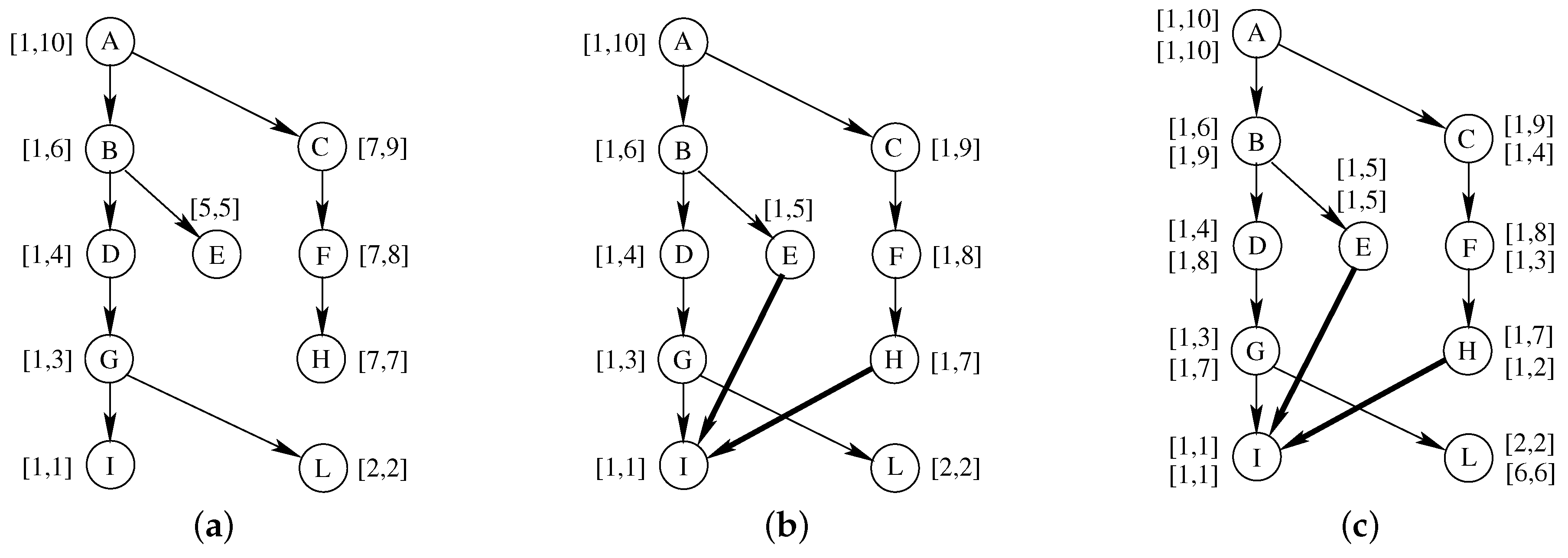
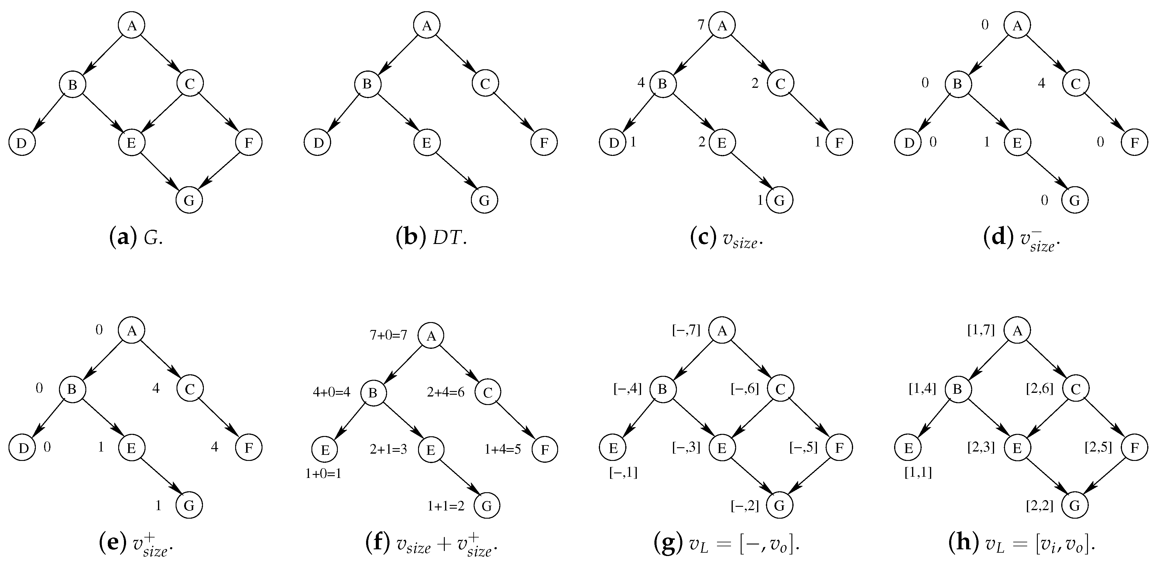
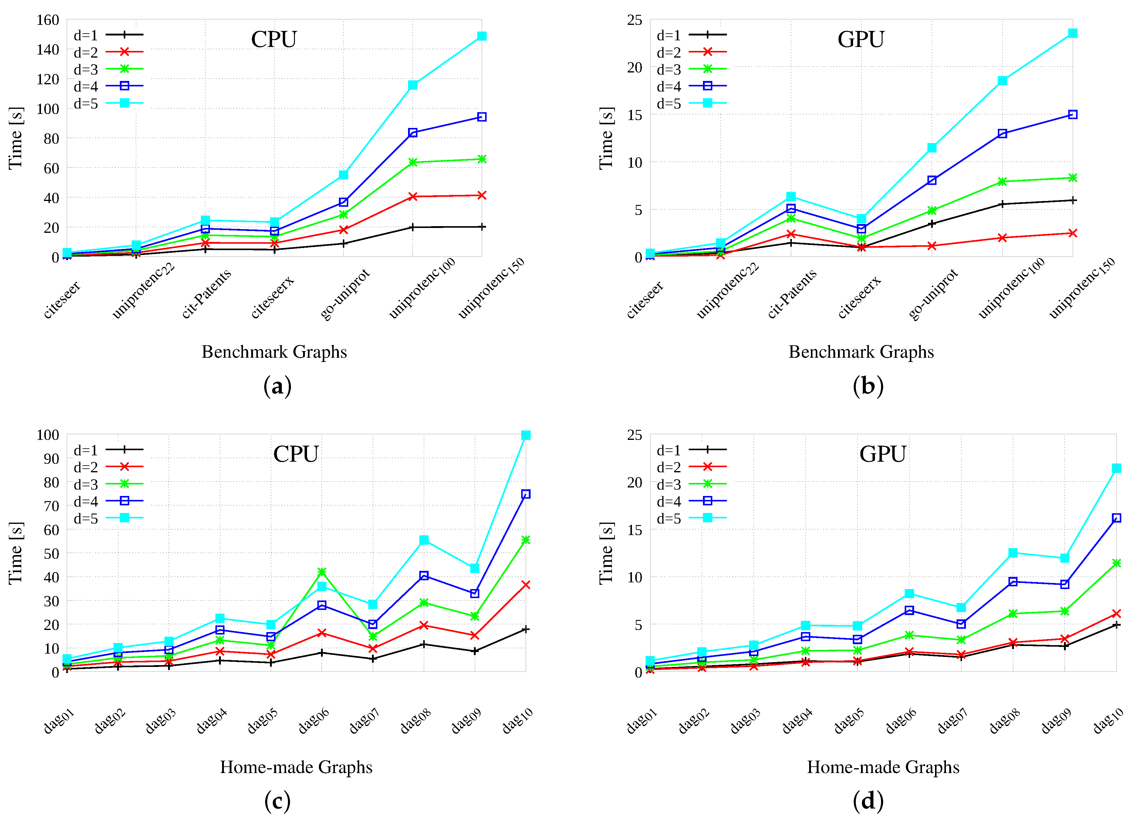
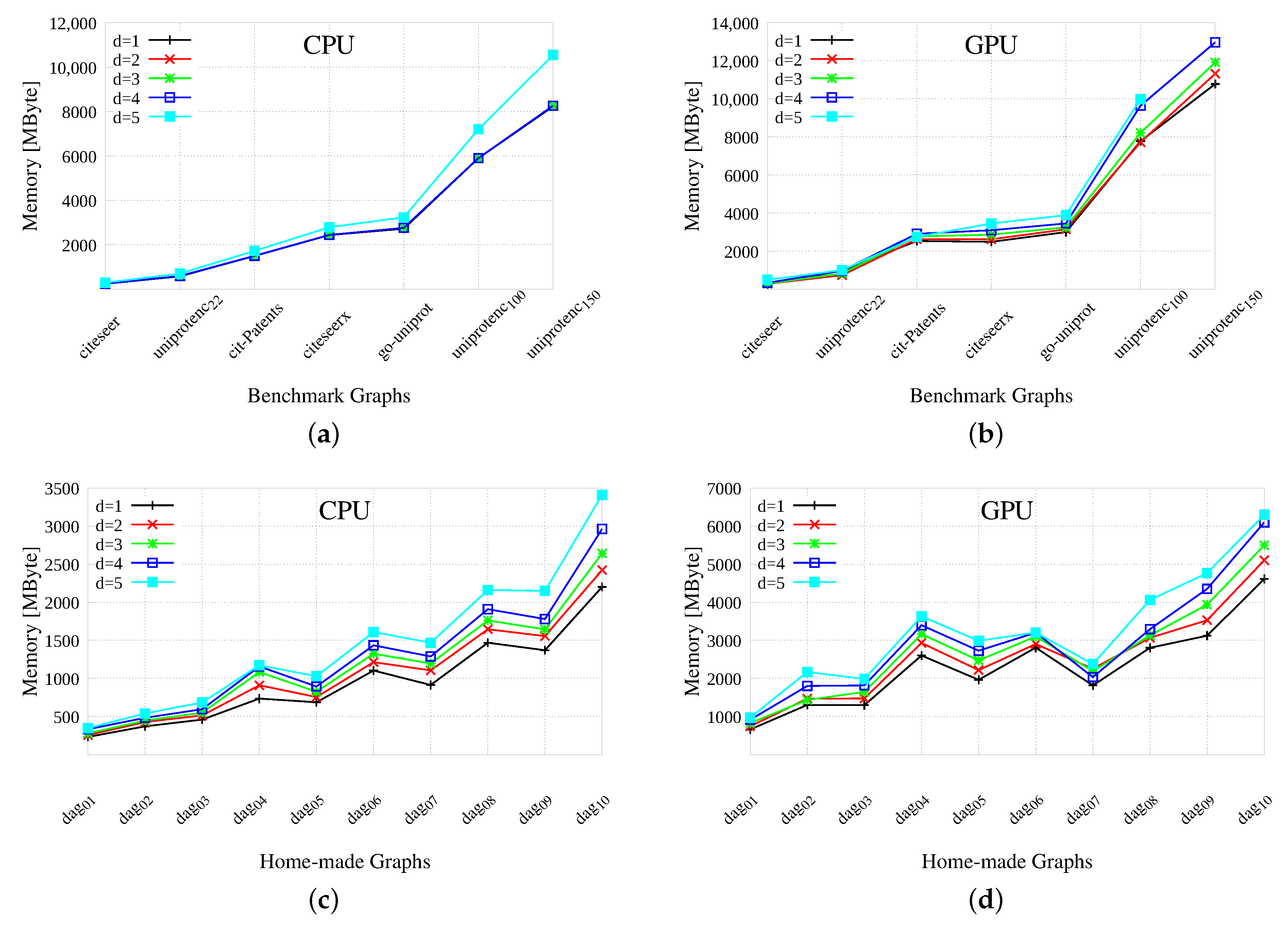
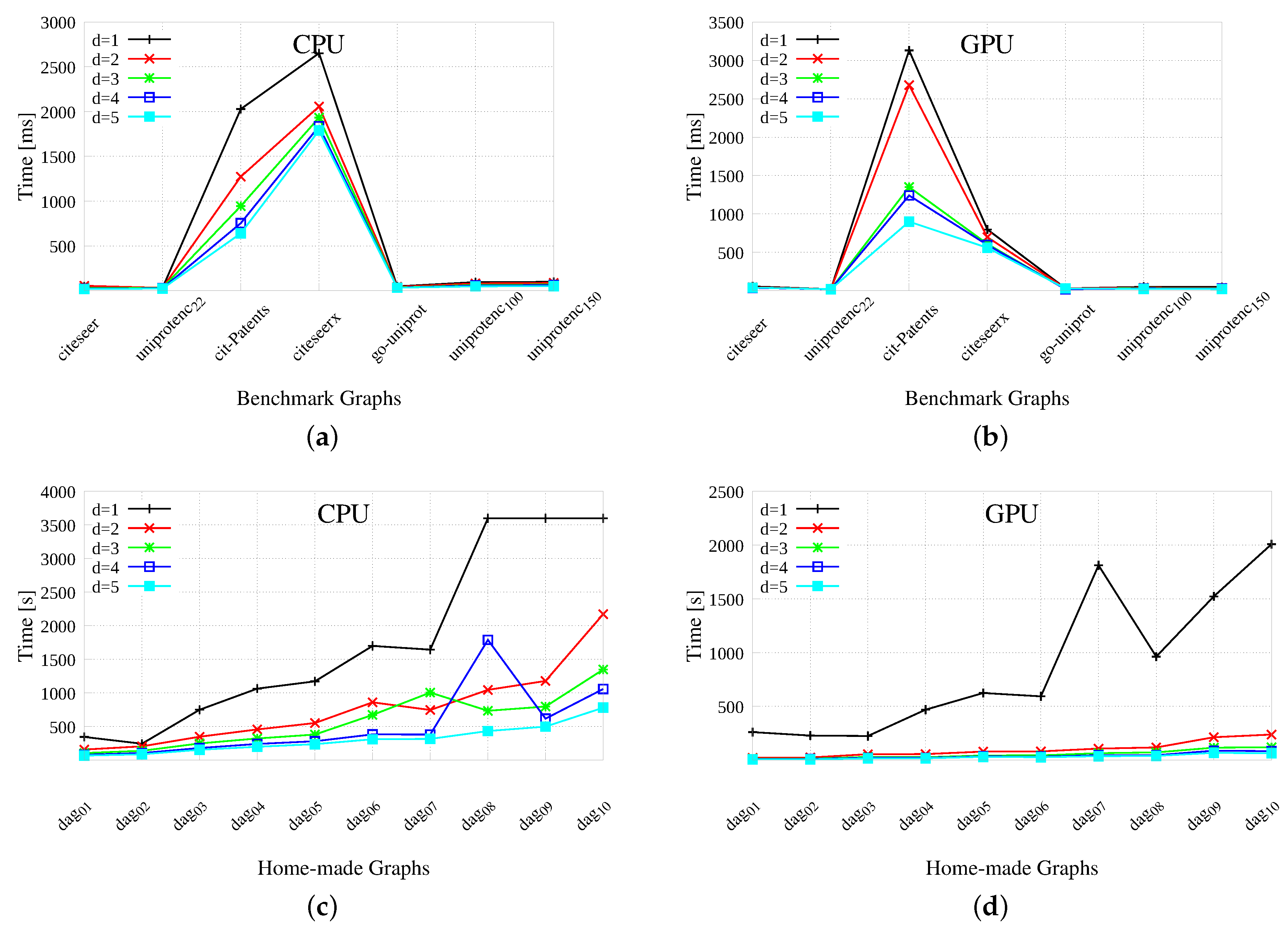
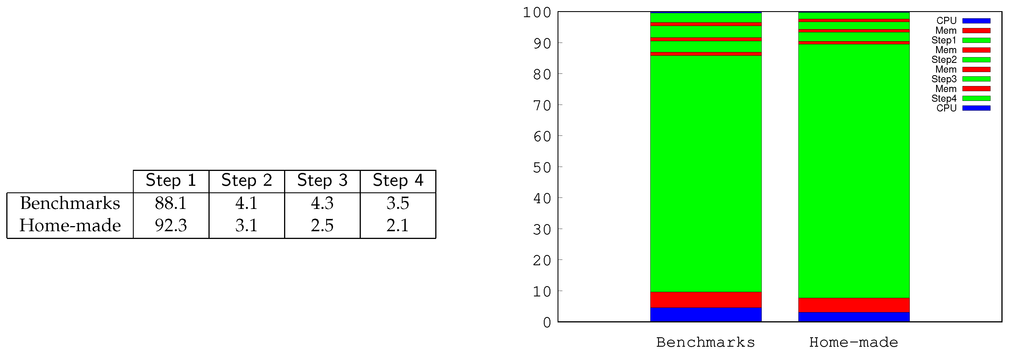
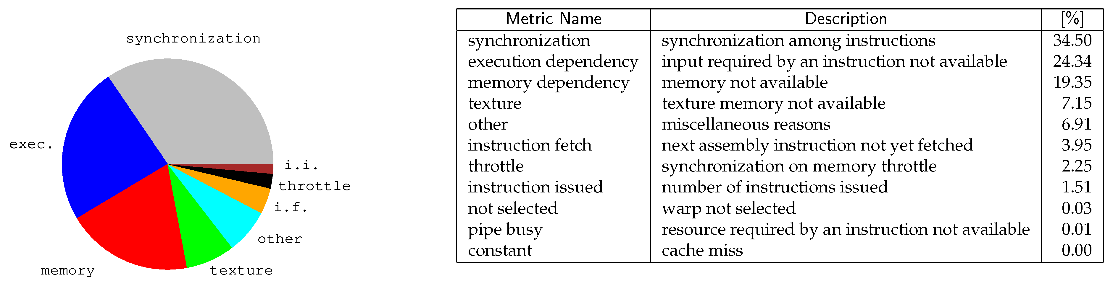
Table 1.
The large benchmark graph set.
| Benchmark | # Vertices (n) | # Edges (m) | Avg. Degree |
|---|---|---|---|
| citeseer | 693,947 | 312,282 | 0.45 |
| uniprotenc | 1,595,444 | 1,595,442 | 1.00 |
| cit-Patents | 3,774,768 | 16,518,947 | 4.38 |
| citeseerx | 6,540,401 | 15,011,260 | 2.3 |
| go-uniprot | 6,967,956 | 34,770,235 | 4.99 |
| uniprotenc | 16,087,295 | 16,087,293 | 1.00 |
| uniprotenc | 25,037,600 | 184,670 | 0.01 |
Table 2.
The home-made graph set.
| Benchmark | # Vertices (n) | # Edges (m) | Avg. Degree |
|---|---|---|---|
| dag | 250,000 | 12,518,774 | 50.08 |
| dag | 250,000 | 24,987,505 | 99.95 |
| dag | 500,000 | 24,959,258 | 49.92 |
| dag | 500,000 | 49,918,815 | 99.84 |
| dag | 750,000 | 37,552,465 | 50.07 |
| dag | 750,000 | 75,003,619 | 100.01 |
| dag | 1,000,000 | 50,009,975 | 50.01 |
| dag | 1,000,000 | 99,934,520 | 99.9 |
| dag | 1,500,000 | 75,024,132 | 50.02 |
| dag | 1,500,000 | 149,989,194 | 99.99 |
Publisher’s Note: MDPI stays neutral with regard to jurisdictional claims in published maps and institutional affiliations. |
© 2020 by the authors. Licensee MDPI, Basel, Switzerland. This article is an open access article distributed under the terms and conditions of the Creative Commons Attribution (CC BY) license (http://creativecommons.org/licenses/by/4.0/).
Share and Cite
MDPI and ACS Style
Quer, S.; Calabrese, A. Graph Reachability on Parallel Many-Core Architectures. Computation 2020, 8, 103. https://0-doi-org.brum.beds.ac.uk/10.3390/computation8040103
AMA Style
Quer S, Calabrese A. Graph Reachability on Parallel Many-Core Architectures. Computation. 2020; 8(4):103. https://0-doi-org.brum.beds.ac.uk/10.3390/computation8040103
Chicago/Turabian StyleQuer, Stefano, and Andrea Calabrese. 2020. "Graph Reachability on Parallel Many-Core Architectures" Computation 8, no. 4: 103. https://0-doi-org.brum.beds.ac.uk/10.3390/computation8040103
Note that from the first issue of 2016, this journal uses article numbers instead of page numbers. See further details here.