A QP Solver Implementation for Embedded Systems Applied to Control Allocation


Institute of System Dynamics and Control, Robotics and Mechatronics Center, German Aerospace Center (DLR), 82234 Weßling, Germany
*
Author to whom correspondence should be addressed.
Computation 2020, 8(4), 88; https://0-doi-org.brum.beds.ac.uk/10.3390/computation8040088
Submission received: 31 August 2020
/
Revised: 2 October 2020
/
Accepted: 6 October 2020
/
Published: 13 October 2020
(This article belongs to the Section Computational Engineering)
Abstract
:Quadratic programming problems (QPs) frequently appear in control engineering. For use on embedded platforms, a QP solver implementation is required in the programming language C. A new solver for quadratic optimization problems, EmbQP, is described, which was implemented in well readable C code. The algorithm is based on the dual method of Goldfarb and Idnani and solves strictly convex QPs with a positive definite objective function matrix and linear equality and inequality constraints. The algorithm is outlined and some details for an efficient implementation in C are shown, with regard to the requirements of embedded systems. The newly implemented QP solver is demonstrated in the context of control allocation of an over-actuated vehicle as application example. Its performance is assessed in a simulation experiment.
1. Introduction
Quadratic programming problems occur in various areas, for example in portfolio optimization where the risk-adjusted return shall be maximized [1], in signal processing operations, in audio applications [2], and in machine learning [3]. The efficient and reliable solution of quadratic programming problems (QPs) is essential in the solution of many real-time control problems. Especially, the use on electronic control units and embedded platforms poses challenges, as described in [1,4]. To run on platforms with little memory space, the solver should consist of code with a small footprint that is self-contained and does not depend on external libraries. For the use in real-time applications, a solution must certainly be accomplished within the sampling time, which can be very short depending on the application. So, the solver needs to be reliable and provide a solution even in the case of poor quality data without causing a termination of the algorithm in which the solver is used. Furthermore, the solver needs to be provided in a programming language matching the requirements of safety-critical applications, such as C, which is widely used especially in the automotive sector. A new C-implemented QP solver is presented here. It is based on the dual method of Goldfarb and Idnani [5]. Other solvers are based on the same method, such as the C++ libraries QuadProg++ [6] and qpmad [7] or a Matlab solver named QP [8]. There also exists a Fortran implementation by Schittkowski named QL [9] based on this dual method. Automatic conversion from Fortran to C is available with the f2c program [10]. However, the C code generated in this way, is not appropriate for application on embedded systems, since it relies on external Fortran libraries and consists of many jump statements. Yet, simple control structures provide benefits for the use on embedded platforms since, e.g., loops with a fixed number of iterations and the avoidance of jump statements make it easier to analyze the overall execution of the code and to determine the real-time capability of the code. Moreover, code with simple control structures is easier to maintain if adaptations should be necessary. However, such manual modifications in the f2c-generated code are not advisable, since the converted code is confusing and not well readable. For these reasons, a handwritten well-readable and embedded system suitable C code implementation of the QL solver was developed. This new implementation is called EmbQP. Although the new solver is based on the same approach as the QL solver, it has been implemented completely new. The new solver follows the process of the QL solver [9] only when handling non-positive definite matrices in the objective function of the QP problem. In contrast to [9], the EmbQP solver can also be used to solve QP problems without any lower and/or upper bounds of the solution vector being given. As an application example for the use of QPs, the control allocation problem from [11] is considered. It is included in the context of path following control for DLR’s ROboMObil (ROMO), a robotic full x-by-wire research vehicle [12]. In [11], the QL solver of Schittkowski was used to solve the QP problems. In the work presented here, the new EmbQP solver is used in this application example, and the simulation results of the two solvers are shown and compared.
The QL Fortran routine according to [9] and the underlying algorithm of Goldfarb and Idnani are explained in Section 2. Section 3 details the implementation of the EmbQP solver. In Section 4, the control allocation problem is described. The results of the simulations and the comparison between the QL solver and the new EmbQP solver are shown in Section 5.
2. Description of the EmbQP Algorithm
The new C implemented QP solver follows the dual active set method of Goldfarb and Idnani [5] with some additions from [9]. The algorithm solves the following strictly convex quadratic programming problem:
with a symmetric and positive definite matrix , vectors and , and a ()-matrix , together with representing linear constraints. Upper and lower bounds for the variable are given by and , respectively. The number of all equality constraints is denoted as .
In this implementation, the lower and upper bounds on are treated as additional inequality constraints by an appropriate expansion of and . Then, the number of constraints is adapted internally. However, it is optional to specify such limits, since the EmbQP solver can also handle QP problems without explicit declaration of lower and upper bounds on , where the constraints are thus only given by and . In contrast, the QL solver of Schittkowski always needs the input of such lower and upper bounds, and if a QP without such bounds is to be solved with it, sufficiently large values must be provided.
The QL routine of Schittkowski is based on the dual method of Goldfarb and Idnani, and the implementation of it goes back to Powell [13]. Some important points of the method of Goldfarb and Idnani are described here, whereas a detailed description can be found in [5]. A good summary of this method can also be found in [14]. The method of Goldfarb and Idnani creates optimal approximate solutions, while the value of the objective function is monotonically increasing. The method uses a so-called active set of constraints
which is the empty set at the beginning. During the course of iterations, indices of the constraints are added to so that represents the set of constraints that are satisfied as equalities with the current solution. Indices of inequality constraints can also be removed from if the corresponding constraint is no longer active. The minimum of the objective function subject to the current active set is calculated at every iteration.
For an active set , the subproblem is defined to be the relaxed quadratic programming problem with the objective function of Equation (1) subject to the subset of constraints, which is given by the active set . In every iteration of the algorithm, and are defined to be the solution pair if the following conditions are fulfilled: the vectors are linearly independent, the relaxed problem is feasible, minimizes the objective function , and satisfies all constraints in with equality. With these definitions, the basic principle of the method of Goldfarb and Idnani can be described. It comprises the following steps in Table 1.
Since the active set represents the empty set at the beginning of the algorithm, yields the minimum of the problem Equation (1) in the unconstrained case (), which is the minimum of the bare objective function. It serves as a starting point, and the first solution pair is given by . The iteratively calculated solution points are inadmissible except for the last one; therefore, there is no need to search for a feasible starting point with the dual method in contrast to other primal active set methods.
The algorithm terminates either after finding the optimal solution of the problem Equation (1) or after detecting that the problem is infeasible. The termination occurs after a finite number of steps, since the number of possible solution pairs is finite and since the return of the algorithm to a formerly computed solution pair is not possible, because the values of the objective function are monotonically increasing from one iteration to the next. The number of the solution pairs is limited by the number of possible subsets of , which is at the most. A reliable upper limit of iterations is particularly important for the use in hard real-time applications.
With a solution pair from the last iteration and a newly chosen violated constraint , two possible cases can occur. Either the vectors are linearly independent or is linearly dependent on . Based on these cases, the index can either be added directly to the active set or an element, which is no longer considered active, has to be removed from first before adding to it. The index is in any case added to .
A short summary of the algorithm of Goldfarb and Idnani is given in Table 2 where, in comparison to the basic principle in Table 1, particularly the computation of a new solution pair is described in more detail. The description of the algorithm is based on [5,14]. The notation is used here to describe a reduced matrix composed only of the rows of whose indices of the corresponding constraints are included in the current active set .
The algorithm takes steps in the primal and dual space, which means in the primal and dual variables, so changes in and/or in the Lagrange multipliers of the corresponding dual problem occur [5]. The dual feasibility is always fulfilled, producing the primal optimality of the subproblems in each iteration. Primal feasibility, i.e., compliance with all constraints, applies only to the last, optimal solution point. A change in the active set and in the dual variables is possible without changing ; see step 6 in Table 2.
The algorithm detects, on the basis of the step length, whether a new constraint can be added to the active set or whether an active constraint has to be removed first from the active set, i.e., whether a full step or a partial step is taken. If a step violates the dual feasibility, it has to be shortened. More details about the implementation of this method in the EmbQP algorithm are described in the next section.
3. EmbQP Implementation Details
Table 3 shows a summary of all inputs and outputs of the EmbQP solver. Further outputs are conceivable and easy to provide, such as the final active set that includes the indices of all constraints satisfied with equality by the solution vector.
In comparison to Table 2, the EmbQP solver implementation requires additional inputs that need to be specified in the calling function. These include Boolean parameters and that determine whether upper or lower bounds for the solution vector are provided or not. In contrast to the Fortran QL solver, the EmbQP solver also works if no upper or lower bounds or only either of them are given. Another additional input is the desired accuracy . It is used for comparisons of variables with zero and should therefore be greater than the target machine precision. Furthermore, as it is the case with the Fortran QL solver, the integer input parameter needs to be specified. It determines whether an initial Cholesky decomposition of is already known from the start and can be provided by the calling function. If this is the case, the provided factorization is stored in the lower triangular part of , and consequently, it is possible to save redundant Cholesky decomposition in the algorithm. When programming code for the use on embedded systems, dynamic memory allocation should be avoided. Wherever possible, the input arguments of a function are overwritten with internal calculations and output arguments to effectively use the available memory. Moreover, a function may need additional temporary memory for internal calculations. To overcome recurrent dynamic memory allocation, pointers to pre-allocated working arrays with an appropriate length and data type are passed to the function. The EmbQP code uses two working arrays, one for float-type data and one for integer-type data. Their size depends only on the dimensions and . The C code segment, where pointers to the integer working array are set, is shown in Table A1. Turning to the outputs, the optimal solution is returned as the main result. Moreover, the minimal objective function value is provided and an integer is returned. The latter reports whether the optimization was successful. This is the case if and only then do the other outputs have reasonable values. The case reveals an infeasible problem, and the case occurs if the maximal number of iterations is exceeded. This last case may only arise due to rounding errors, since theoretically, with infinite precision, the algorithm will always find an optimal solution or detect the infeasibility of the problem. In the cases or , the EmbQP algorithm does not deliver meaningful values for and , but it ensures that the solution returned for is within the bounds and . Table A2 shows how this is done in the C code in the case of an unfeasible problem. So, at least these constraints are always fulfilled as long as they represent applicable boundaries. A C main function in Table A3 shows data for an example QP problem and how the EmbQP solver is called with the above-mentioned inputs and outputs.
The matrix in the objective function of Equation (1) needs to be symmetric and positive definite in the original algorithm. The routine of Schittkowski can also handle positive semidefinite matrices that may occur as a consequence of rounding errors or other numerical deficiencies. This approach is also adopted in the EmbQP solver. At the beginning of the algorithm, a Cholesky decomposition of is carried out (if not already provided), and during this factorization, a non-positive definite matrix can be identified. In this case, the identity matrix multiplied by a small factor is added to the matrix to increase its diagonal elements. is increased iteratively until a positive definite matrix is obtained for which the Cholesky decomposition can be performed. In this situation, a quadratic programming problem with a slightly perturbed objective function with instead of is solved. Based on [13], the value of and the perturbed are computed using the elements of the already calculated decomposition matrix as well as the pivotal element that caused the break of the decomposition. It is ensured that is positive and increases its value in each step so that the procedure converges and provides a small value that gives positive definiteness.
Several options are possible for the choice of the violated constraint to be added to the active set. The successful termination of the algorithm does not depend on this choice, so one has the freedom of choosing any violated constraint. However, by an adapted choice, the number of iterations may be reduced. A simple possibility with no additional computation is the choice of the violated constraint with the lowest index. An alternative that might be more effective is to choose the most severely violated constraint. Different strategies for this choice, for example the computation of euclidean distances, can be found in [15]. In the implementation of the EmbQP solver, two possibilities were tested: in one case, the violated constraint with the lowest index was used, and in the other case, the most violated constraint was chosen. The latter one is the constraint for which the absolute value of the residual is the greatest, with a violated constraint from Equation (1). The results for both variants were equivalent in terms of ; however, the first variant required more iterations until the optimal solution was found, which led to a longer computing time. For this reason, the second option was used for the results presented in Section 5. The corresponding segment of the EmbQP code selecting the violated constraint is shown in Table A4.
Table 4 shows a pseudo code of the EmbQP algorithm, using the method in Table 2 and the input arguments of Table 3.
Since the computation of the step sizes and and the dual variable was taken from [5,14] and does not present any particular challenges for the implementation in C, it will not be addressed further here. However, the computation of the two matrices and , is an essential part of the algorithm and can be time-consuming if it is not done efficiently. It is explained in more detail in the following.
At every iteration of the algorithm, directions in the primal and dual space are computed by means of matrices and as specified in Table 4 and step 3 of Table 2. However, a direct evaluation of these matrices is not efficient. These matrices depend on the active set , which differs only by one element from step to step because either an element is added to the active set or an element is removed from it. Taking advantage of this feature enables updating of the matrices and . Updating the appropriate decompositions of and reduces the effort for computing the step directions even more. The approach described in the following is based on [5,14]. At the beginning of the algorithm, the Cholesky decomposition of the objective function matrix is carried out, , and also the inverse of the lower triangular matrix is computed:
For updating and , we assume that there exist matrices and with the following characteristics:
with and an upper triangular matrix , where is the number of elements of the current active set . The matrix can be partitioned into two submatrices
where comprises the first columns of and comprises the last columns. By exploiting this and substituting Equations (3) and (4) in the definition of the matrices and in step 3 of Table 2, we obtain
Therefore, the matrices and can be expressed by means of the matrices and . By defining the vector
where is the row of the matrix with the index , the vectors and can be expressed as and . Since is an upper triangular matrix, the vector can be easily calculated by backwards substitution. So, for computing the step directions, there is no need to determine the matrices and in every iteration. Updating and is sufficient and comprises all needed information. At the beginning of the algorithm, the active set is empty and . By choosing with from Equation (2), the prerequisites from Equation (3) are fulfilled in the first iteration of the algorithm. In the next steps, the updated matrix is calculated by means of an orthogonal matrix as
This approach can be used for both cases in the iteration, i.e., both when an element is added to and when an element is removed from it. If an element is added to , the matrix can be composed in this way:
The matrix denotes the identity matrix in the . With this approach, it follows with Equations (3) and (6):
Since the assumptions in Equation (3) must also be fulfilled in the next step, it follows that the matrix must be chosen in a way that the product is collinear with the first unit vector in the . This can be achieved using Givens rotations. Thus, the matrix is a product of Givens rotations. They are successively multiplied with and eliminate one component of the vector at a time, until finally becomes collinear with the first unit vector. With
the matrix needs to be successively multiplied with the Givens rotations. For , it is:
where denotes the first component of . With (10) and (11), the matrices and can be updated by successively multiplying and with Givens rotations. These multiplications can be performed in one step in direct succession so that the Givens matrices do not have to be stored in each step, and the matrix does not have to be calculated explicitly. In case an element is removed from the active set , the same approach in Equation (7) can be used. We assume that the element is removed, which is located at the position of . The operator is defined to remove the row of a matrix. With that, it is:
Using Equation (12) and the prerequisite from Equation (3), the following applies:
The operator removes the th column of . The matrix can be divided in submatrices:
with the upper triangular matrix , and . Since is an upper triangular matrix, is an upper Hessenberg matrix. The matrix is chosen as follows:
where and are identity matrices and is an orthogonal matrix. Using Equations (15) and (14) in Equation (13) yields:
From that, it follows that has to be chosen in a way that the product becomes an upper triangular matrix. Again, Givens rotations are used. Therefore, the matrix is a product of Givens rotations, which are successively multiplied with . Turning to the matrix , we again use the partition from (4) and divide the matrix into two further submatrices:
with und . With Equations (15) and (17), it is:
In , only the columns to differ from . The matrix is multiplied with the same Givens rotations as . This can again be carried out in parallel and without the need to explicitly determine the matrix . With the described approach, the updating of the matrices and can be done efficiently, both when an element is added to the active set and when an element is removed from it. All required algorithms for these computations, such as the Cholesky decomposition, Givens rotations, or backwards substitution, were implemented in C. The C function for computing plane Givens rotations used within the EmbQP solver is shown in Table A5. As a consequence, the EmbQP algorithm is self-contained, and no external library is needed.
Furthermore, the C code was written in a way that adheres to the coding guidelines of Motor Industry Software Reliability Association (MISRA) [16]. These guidelines aim at improving the quality of the C code by using only a subset of the C language with the objective of decreasing the incidence of undefined or unpredictable behaviors and of enhancing the reliability and maintainability of the code. In the automotive industry and safety-critical applications, the MISRA-C guidelines are established and typically required with the programming of embedded systems. One issue that comes up with the observance of the MISRA guidelines is the handling of input values from external sources. Their validity needs to be checked at the beginning of the algorithm. Another issue is the avoidance of dynamic memory allocation, which is resolved by the use of working arrays in the EmbQP code. Furthermore, the basic data types of C shall not be used directly. They are only allowed in type definitions. Thus, for each variable, the appropriate data type is defined according to its respective properties. Another example for the rules of the MISRA guidelines is the aspect that only one return or break statement is allowed to terminate an iteration. This was respected with the while loops in Table 4 and implemented with additional if constructs. In summary, the EmbQP code was written in a way that respects the MISRA guidelines that are often required for safety-critical applications in the automotive sector.
4. Application of the EmbQP Solver in a Vehicular Control Allocation Problem
As an application example, the EmbQP solver is used as a part of a control allocation algorithm in the context of path following control. The problem formulation goes back to [11,17,18]. A short overview about the control allocation is given in this section.
4.1. Control Allocation Problem
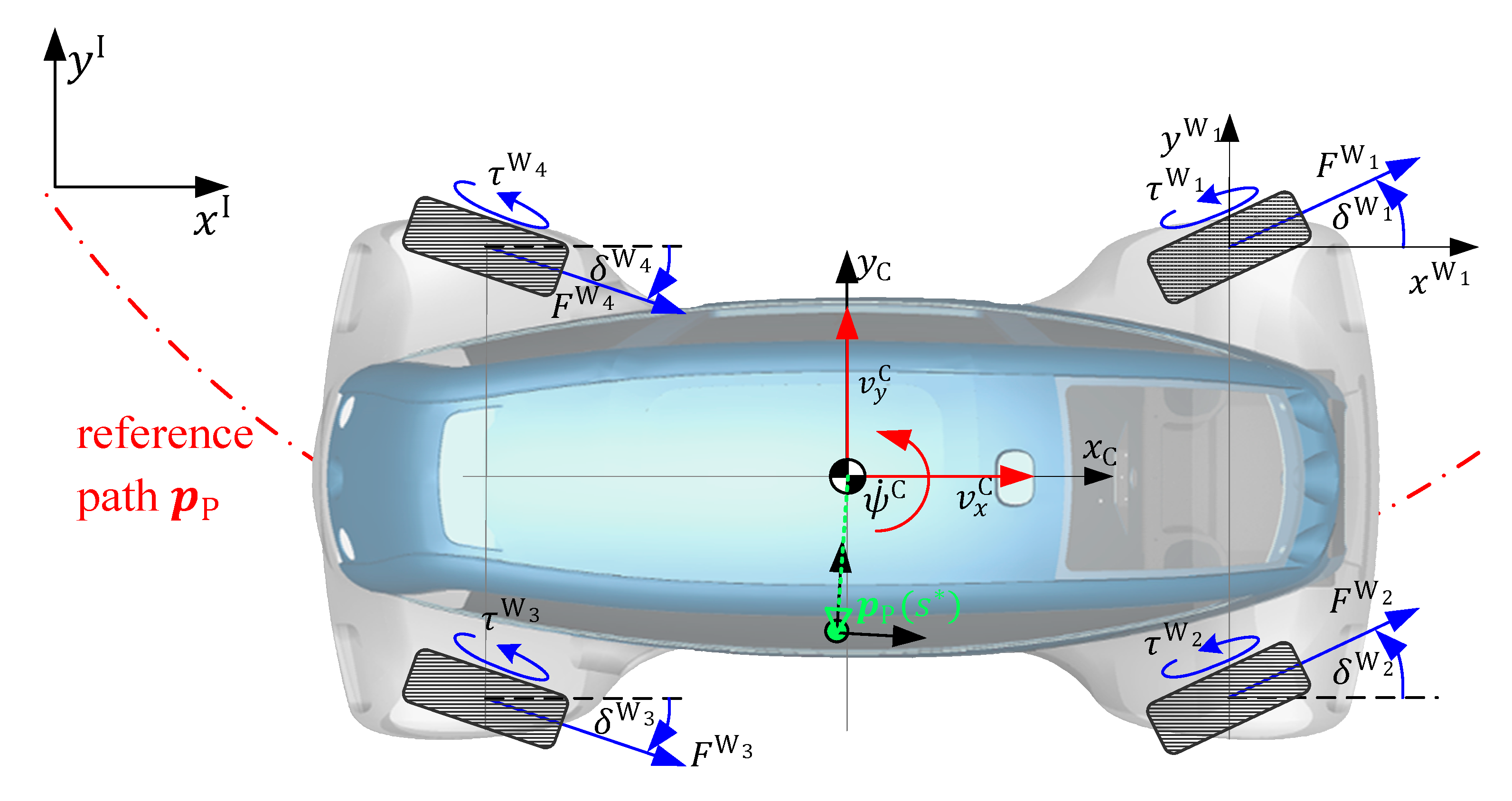
Path following control is an example of motion control, and it plays an essential part in the development of autonomous vehicles. Path following control affects the movement of a vehicle with the aim that it follows a predetermined path with only small lateral displacement. The considered vehicle is the ROboMObil (ROMO) [12], which is a robotic full x-by-wire research vehicle featuring four almost identically constructed wheel robots. Its planar movement can be directed by setting the steering angles of the four wheels and the drive torques of the in-wheel motors. These control input variables of the vehicle are described by the eight-dimensional vector :
In many control systems, the number of virtual control inputs to the mechanical system equals the number of degrees of freedom [19]. In contrast, the ROMO belongs to the class of over-actuated systems. It has three degrees of freedom of the horizontal motion but eight control inputs. The desired motion is represented by three so-called virtual control demand variables being the longitudinal, lateral, and rotational velocity at the vehicle’s geometric center:
The configuration of the ROMO with its four wheels and the above-mentioned variables is shown in Figure 1. The arc length on the reference path is the one that minimizes the displacement between the vehicle position and the path position . The determination of is done by using a time-independent path interpolation as described in [11].
In the real-world application, the vehicle states can be estimated e.g., as proposed in [20]. Since there is no unique actuator available that directly meets the virtual control demands , a control allocation is necessary to determine and distribute the commands that are applied to the physical actuators. So, the control allocation serves as an interface between the controller and the available actuators of the vehicle and maps the computed virtual control demands to the physical control inputs .
The primary goal of the control allocation is to achieve the desired virtual control variables if feasible. A secondary goal is to find an energy-friendly solution in a way so that simultaneously, the instantaneous total power consumption should be minimized while satisfying the desired motion. For solving this problem, an optimization-based method is applied. The goal is to minimize a certain objective function while considering the solution of the control allocation problem and the physical actuator constraints. The objective function can be formulated as a heuristic cost function, which should meet the following two goals for reaching low energy consumption: The steering rate should be minimized to avoid mechanical losses and the traction motor torque should be chosen so that recuperation is maximized. These two rules are conflated in a cost function that can be adjusted offline, and since it represents a simple function expression, it is suitable for real-time applications [17]. One approach for minimizing an objective function for the actuating variable variation is a two-step optimization:
First, a set of physically feasible solutions is found that respects the actuator limits and in each time step. is a weighting matrix to prioritize the virtual control variables , and denotes the control-efficiency matrix for the linear relation between the virtual control variables and the actuating variables. is the sample time in a time discrete system. If there exists a manifold of solutions in the first step, then the second step seeks for a solution in the manifold that minimizes the objective function .
4.2. QP Problems in the Control Allocation
The energy optimal control allocation problem is solved using quadratic programming. The EmbQP solver is employed here. Therefore, the steps in Equation (21) that represent a least squares minimization problem need to be rewritten to obtain a quadratic programming compatible problem in the form of Equation (1) [11]. The transformation by matrix computation leads to the following equivalent formulation of the first step of Equation (21):
The weighting matrix for the virtual control inputs is defined at the beginning of the algorithm and remains the same in each time step. The configuration of the control-efficiency matrix depends on changes of states or inputs. However, during the current sample interval, it remains constant, and the QP Equation (22) can thus be treated as a static problem [19]. Then, the matrix is recalculated in each time step using the current vehicle speed and yaw rate and the current settings of the actuator variables; so, the problem is solved with a new matrix in the next time instance. The upper and lower bounds and define the physical limits for the actuating variables. They are recalculated in each time step and may vary depending on the current state of the vehicle. The virtual control variables are passed on to the control allocator by the controller.
The problem (22) is the first of two QPs that is solved in each time step within the control allocator. It represents the actual control allocation and means that a solution is sought that minimizes the distance between the virtual control demands and the real actuator motions subject to the physical limits, compare step 1 of (21). Next, the computed solution is used to check if there is a nullspace. Considering limited numerical accuracy, practically, this is true if holds for a small value . If a nullspace exists, there is a manifold of solutions in terms of to achieve the virtual control demands. Accordingly, the additional goal of low power consumption is inserted as described in the second step of (21). It also needs to be reformulated as a QP problem. In the cost function that seeks for energy optimality, the difference between the actuating variable and the demand are to be minimized. The demand represents the goals formulated above for the steering rates and the motor torques. The former are set to zero, while the latter are chosen to achieve the maximal available recuperation depending on the current state of the vehicle; see [11]. So, the cost function results in with a weighting matrix for the control signals. Again, matrix computation yields a QP formulation for this optimization:
This is the second QP problem that is solved in each time step but only if the solution of (22) shows that there is a nullspace. If no nullspace exists, there are no physically admissible actuation control variables that can reach the demand of the virtual control variables. So, there is no intersection between the set of admissible solutions and the set of virtual control variables. Nevertheless, the actuating control variables need to be specified in each time step of the control allocation algorithm. So, a solution is sought that minimizes at least the distance between these two sets and preserves the direction of the virtual control variables. The following QP problem is solved if there is no nullspace:
This QP formulation is similar to the first one in Equation (22). In comparison to (22), the weighting matrix is neglected, which is chosen as the identity matrix in our application example anyway. The objective function is supplemented by a diagonal matrix . With large entries in the first four diagonal elements compared to the last four ones, it makes sure that the steering angles do not deflect too far from the set-point.
Table 5 shows a pseudo code of the steps in the control allocation with the three calls of the EmbQP solver.
Details about the design of the lateral and the longitudinal controller, which compute the virtual control variables, can be found in [11] as well as further information about integrating the control allocator into the path following control. In addition to the calculation of the matrices and vectors for the QP problems, there is a dynamic calculation of the maximum actuating variables in each time step, which takes into account the current states of the actuators.
A check is inserted after the optimization steps of the control allocator to verify whether the computed solution is within the admissible range specified by the physical limits and . If that is not the case, the solution is clipped to the admissible set. This check should not be necessary, but nevertheless, it is included as a precaution if an error during the optimization is not detected.
In summary, in each time step of the motion control algorithm, two QPs have to be solved within the control allocation. The first QP (22) is solved in each time step and depending on its solution, either the QP (23) or the QP (24) is solved, while the solutions of the latter QPs are the output of the control allocator and used as actuator set-points in the next time step. Details about the implementation and the numerical results are given in the next section.
5. Results of the Simulation
In this section, the EmbQP solver is assessed against the Fortran QL solver [9] by means of comparative simulations of a path-following scenario with the ROMO. While using the Fortran QL solver, version 3.2, these simulations were already accomplished in [11], which facilitates the comparison. The total simulation model comprising a complex vehicle dynamics model of the ROMO, the path-following control, and the control allocation-based motion control was established in [11] using Modelica, an object-oriented modeling language for multiphysical systems, see [21], and the software tool Dymola. Details about the modeling of the ROMO and the multiphysical Modelica components can be found in [11].
For the comparison, the Fortran QL solver now only needed to be replaced by EmbQP, which is easy to accomplish, since both solvers can be interfaced into the Modelica environment using so-called external C functions. In the case of the Fortran QL solver, the Fortran code had been automatically converted from Fortran to C beforehand using f2c [10]. The two solvers are compared with respect to the following criteria: the course of the solution vectors, the adherence to the constraints, the minimal objective function value, and the computing times.
The three matrices in the objective functions to be minimized in Equations (22)–(24), respectively, are chosen in a way that they are symmetric and either positive definite or positive semidefinite. In the latter case, a small multiple of the identity matrix is added to the positive semidefinite matrix during the optimization to obtain a positive definite one, as described in Section 3.
The predefined path the vehicle should follow is specified by means of a look-up table used for interpolation. The simulation is performed for a path with a length of about 3083 m and with a sampling time of 0.004 s. Figure 2 shows results of both the EmbQP solver and the QL solver for the QPs (23) and (24) for the fifth component of the eight-dimensional solution vector from (19), which is the drive torque for the front left wheel. In Figure 2a, which shows the results for the entire path, there is hardly any difference to be observed between the two solutions. Figure 2b shows a closer look at the first few steps of the simulation revealing discrepancies.
The differences are due to the fact that the two solvers do not solve the very same QPs in each time step. The EmbQP and the QL solver both are based on the same algorithm of Goldfarb and Idnani, but they represent different implementations in different programming languages. One difference is that the QL solver provides a separate handling of the lower and upper bounds [9], while the EmbQP solver considers the bounds identical to the other linear constraints. Consequently, the two solvers provide slightly different results of the optimization. The two simulations, one with the QL solver and one with the EmbQP solver, have only in the first time step the same QP problem to be solved. The slightly varying results of the two solvers are used further and lead to a different position of the vehicle in the next time step and thus to different QPs that need to be optimized in the following time steps. Thus, slight differences in the solution of the solvers as in Figure 2 are expected, since they solve different QPs, which impedes a comparison of the two solvers. Therefore, the comparison of the solvers has been carried out in a different manner for the following figures: both solvers solve the corresponding QPs in one time step, but only one solution is used for the next time step, and so on. To be more specific, in one simulation, the solution of the EmbQP solver is used for feedback in the next step of the motion control, while the QL solver also calculates solutions for the QPs, but these solutions are only used for comparison but are neglected for feedback. For a second simulation, it is done the other way round. With this proceeding, a better comparison of the two solvers is possible, because they solve QPs with the same input data in each time step.
First, the solution provided by the EmbQP solver is considered, while the QL solver runs simultaneously and solves the same QPs for a comparison.
Figure 3 shows the solutions of the two solvers obtained in this way for the QPs (23) and (24). The first and the fifth component of the solution vector from (19) are depicted. The results for the four steering angles and the four torques are similar, which is why only one component of each is shown here for better clarity. Figure 3 also shows the lower and upper bounds for the respective component. It is noticeable that the solutions of both solvers remain within the limits and are very similar. Zooming in, as in Figure 2b, does not result in both lines being visible separately, as they are close to each other. Therefore, the absolute difference is also plotted on a logarithmic scale. It is very slight and illustrates that both solvers find very similar solutions for these QPs.
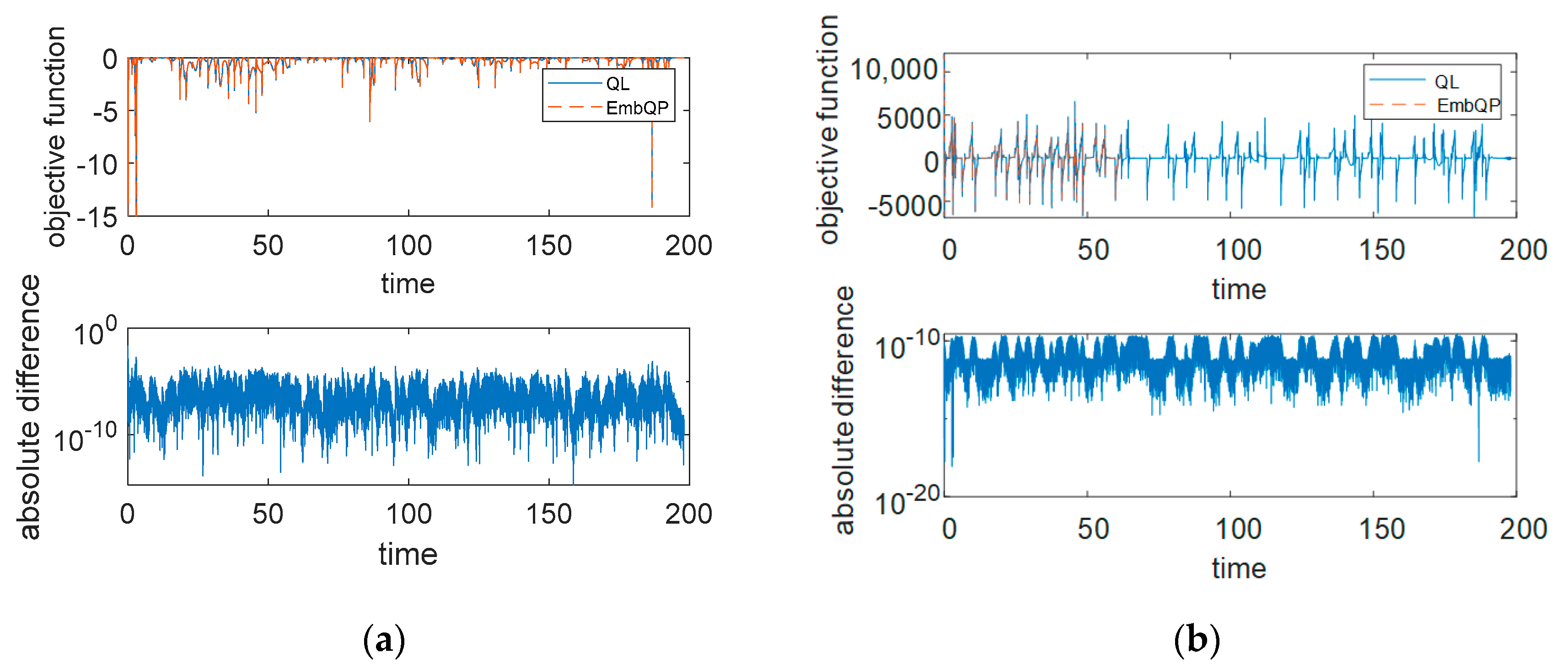
Figure 4 shows the optimal objective function value of the two solvers for the first QP (22) and the two QPs (23) and (24) as well as their respective absolute difference on a logarithmic scale. Since the solution vectors for QPs (23) and (24) are very similar, it is consequently also the objective function value. For QP (22), there are slightly larger differences.
The results mentioned above are obtained with the solution of the EmbQP solver, while the QL solver only runs in parallel and solves the same QPs in each time step. As a second simulation, the other way round is performed; that means the solution provided by the QL solver is considered, while the EmbQP solver runs simultaneously to solve the same problems and to enable a direct comparison. The solutions of the two solvers for the QPs (23) and (24) are very similar to the solutions in Figure 3 and therefore are not shown here. Both solvers keep the limits, and again, the absolute differences between the two solvers are very small. The same holds for the objective function values corresponding to Figure 4.
The C code was compiled using the Microsoft Visual C++ 2017 compiler. The test system on which the simulations were performed is a laptop with Intel i9-9980HK CPU @ 2.40GHz and 32GB RAM with Windows 10 (64 Bit) as operating system. The two solvers perform very similarly regarding the computing times. For this, the simulations have been carried out with only one of the solvers at a time. The simulation using the integration algorithm Dassl in Dymola yields an overall computing time of about 64 s for both solvers with a CPU time of about 1.3 ms for one grid interval of the simulation. Thus, the time for the simulation of one interval is considerably less than the sampling time of 4 ms. Since this simulation also includes the path-following controller and the vehicle model, the low computing time indicates the real-time capability of the solver.
6. Outlook: Configuration of a QP-Based Controller Software on an Embedded Platform
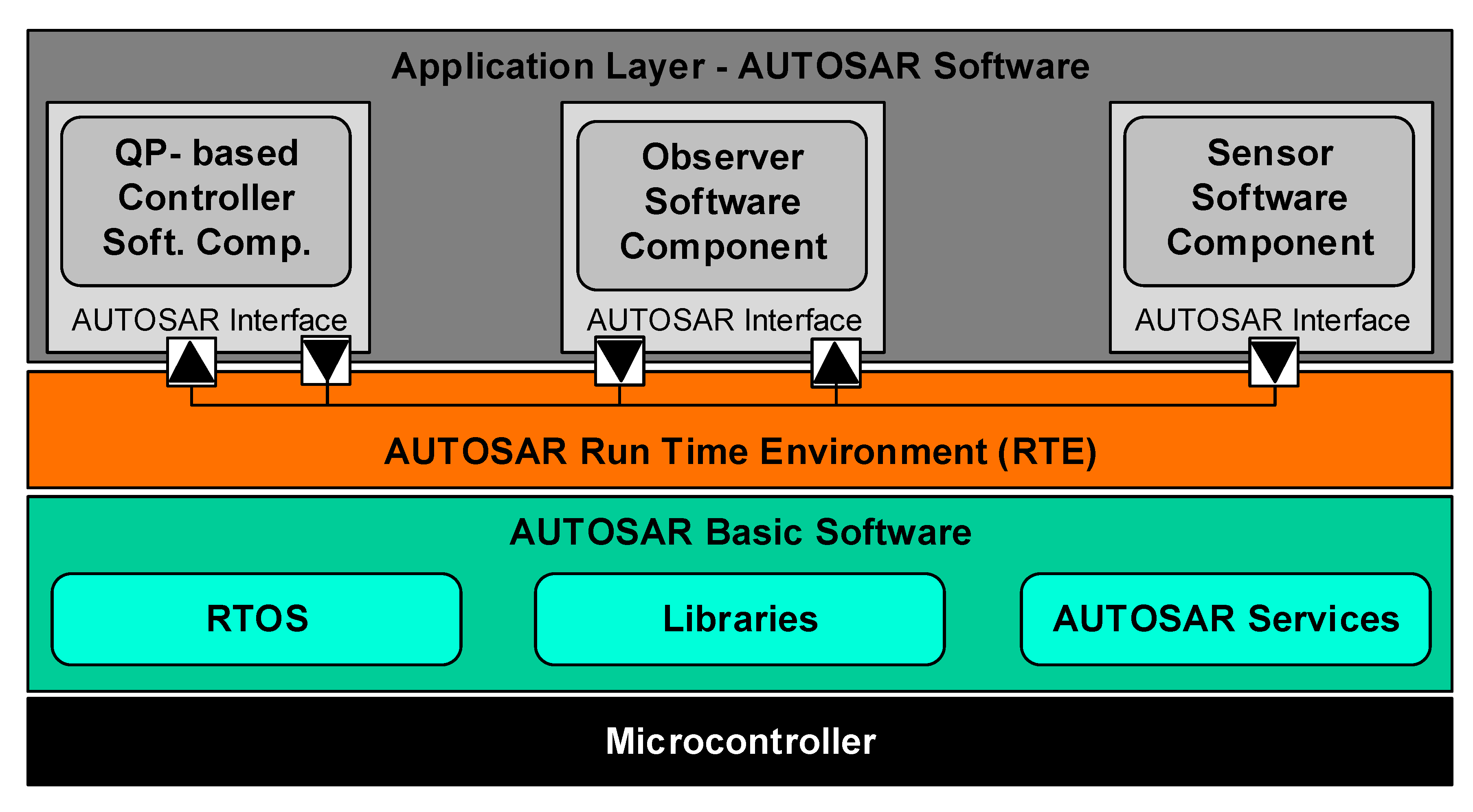
In the following, a short overview is sketched using the EmbQP solver as part of a software application on an embedded platform. As one possible environment, the automotive open system architecture (AUTOSAR) standard is chosen that is widely used in the automotive sector. In [22], a corresponding configuration for a cell battery observer on an embedded microcontroller is shown. It is based on [23], where an integration of the Functional Mock-up Interface (FMI) in AUTOSAR software is proposed. The approach in [22] can be adapted for the usage of an application example with the EmbQP solver. The overall scheme is shown in Figure 5.
The lowest layer of this AUTOSAR layered architecture represents the hardware, which is a microcontroller here. It receives inputs from sensors and passes electrical signals to the actuators. The next layer summarizes the AUTOSAR basic software. It integrates a real-time operating system (RTOS) and some libraries e.g., for integration algorithms. This layer provides the infrastructure services for the top layer of the diagram that is the application layer. The top layer and the AUTOSAR basic software layer are interconnected by a runtime environment (RTE). The application layer incorporates all software components that are necessary for the respective application, such as a sensor and controller software. The observer software handles the estimation of the vehicle states, as described in [20]. The software components can be deployed as Functional Mock-up Units. The EmbQP solver is integrated as a part of the control allocation within the controller software component in the application layer. The data exchange between different software components as well as between the application layer and the basic software layer is performed by the RTE using *.arxml files. The latter are described in detail in [23]. The software components are evaluated periodically and have to meet the real-time conditions. The entire inter-process communication and also the handling of interrupts is performed by the RTE. The described approach with the separation between the application and the hardware provides the advantage of incorporating new models or algorithms on an embedded platform without the need for detailed expertise about the AUTOSAR structure or the used hardware due to the standardized procedure.
7. Conclusions
In this work, a new solver for quadratic programming problems named EmbQP has been introduced. It is based on the dual method of Goldfarb and Idnani, and it is similar to an existing Fortran implementation named QL. The new solver was implemented completely new in the programming language C with the demand of eligibility for embedded systems and safety-critical applications in the automotive sector. The C implementation is mainly based on [5,14], but two aspects of the implementation go back to the Fortran QL solver. These are the option that a previously known Cholesky decomposition of the matrix can be passed to the algorithm and the handling of a non-positive definite matrix in the objective function. In the latter case, as described in Section 3, the EmbQP solver follows the very algorithmic steps of the QL solver for computing the certain small factor multiplied by the identity matrix that is added to . In addition, the EmbQP solver also includes two new features. Firstly, the new C solver is well suited for solving a larger variety of QP problems than the Fortran implementation, since it does not require any lower or upper bounds for the solution vector in the formulation of the QP problem. When using the QL solver, appropriate large values must be specified for each QP. If such lower and upper limits are given, secondly, the EmbQP solver ensures that they are always respected as long as they represent applicable boundaries, even in cases where the solver stops without finding an optimal solution, i.e., when the problem is infeasible or the maximal number of iterations is reached.
The EmbQP implementation also applies an efficient updating of matrices by means of Givens rotations. It does not use dynamic memory allocation because working arrays pre-allocated at the initialization time are passed from outside to the algorithm. Furthermore, the EmbQP solver does not employ any external libraries since it is self-contained with all the required algorithms. The new solver also adheres to the MISRA coding guidelines. In the example of a simulated vehicular control allocation problem, the solver was validated and showed good results and performed equally compared to the Fortran solver. Due to these promising results and its efficient implementation, the EmbQP solver is considered suitable for future use on embedded platforms. Respective implementation and testing will be addressed in further research, together with runtime analyses. On series embedded platforms with limited numerical precision, the solver needs to be assessed to remain numerically stable and reliably provide solutions.
Author Contributions
Conceptualization, C.S. and J.B.; methodology, C.S. and J.B.; software, C.S.; validation, C.S.; formal analysis, C.S.; investigation, C.S.; resources, J.B.; writing—original draft preparation, C.S.; writing—review and editing, C.S. and J.B.; visualization, C.S. and J.B.; supervision, J.B. All authors have read and agreed to the published version of the manuscript.
Funding
This work was funded by the DLR internal project NGC-KoFiF.
Acknowledgments
The authors’ thanks go to Tilman Bünte for his feedback and help in scientific writing.
Conflicts of Interest
The authors declare no conflict of interest.
Appendix A. Code Segments of the EmbQP C Code

Table A1.
Code segment where pointers to the integer working array are set.
| int_t* position = &int_workarray[0]; |
| int_t* ind_ineq = &int_workarray[m+n+n]; |
| int_t* ind_viol_constr = &int_workarray[2 × (m+n+n)]; |
| int_t* pos_r_ind = &int_workarray[3 × (m+n+n)]; |
| int_t* pivot = &int_workarray[4 × (m+n+n)]; |
Table A2.
Code segment to set to a value within the bounds if the problem is infeasible.
| if (t_sigmainf == TRUE) {//problem not feasible |
| if (bounds_x_l) { |
| for (i = 0; i < n; i++) { |
| if (x[i] < x_l[i]) { |
| x[i] = x_l[i]; |
| } |
| } |
| } |
| if (bounds_x_u) { |
| for (i = 0; i < n; i++) { |
| if (x[i] > x_u[i]) { |
| x[i] = x_u[i]; |
| } |
| } |
| } |
| *exit = 2; |
| } |
Table A3.
C main function with data of a QP problem and call of EmbQP.
| int main() { |
| //problem data |
| int_t m = 3; |
| int_t m_e = 3; |
| int_t n = 5; |
| real_t C[25] = {2.0, −2.0, 0.0, 0.0, 0.0, −2.0, 4.0, 2.0, 0.0, 0.0, 0.0, 2.0, 2.0, 0.0, 0.0, 0.0, 0.0, 0.0, 2.0, 0.0, 0.0, 0.0, 0.0, 0.0, 2.0}; |
| real_t d[5] = {0.0, −4.0, −4.0, −2.0, −2.0}; |
| real_t A[15] = {1.0, 0.0, 0.0, 3.0, 0.0, 1.0, 0.0, 1.0, 0.0, 0.0, 1.0, 0.0, 0.0, −2.0, −1.0}; |
| real_t b[3] = {0.0, 0.0, 0.0}; |
| real_t x_l[5] = {−10.0, −10.0, −10.0, −10.0, −10.0}; |
| real_t x_u[5] = {10.0, 10.0, 10.0, 10.0, 10.0}; |
| real_t EPS = 1.0 × 10⁻¹²; |
| int_t mode = 1; //a Cholesky decomposition of C needs to be computed internally |
| boolean_t bounds_x_l = TRUE; |
| boolean_t bounds_x_u = TRUE; |
| real_t x[5] = {0.0}; |
| real_t f_min = 0.0; |
| int_t exit = 0; |
| real_t real_workarray[588] = {0.0}; |
| int_t int_workarray[57] = {0}; |
| EmbQP(m, m_e, n, C, d, A, b, x_l, x_u, EPS, mode, bounds_x_l, bounds_x_u, x, &f_min, &exit, real_workarray, int_workarray); |
| return 0; |
| } |
Table A4.
Code segment for selecting the violated constraint .
| //choose the most violated constraint |
| test_any = FALSE; |
| numb_viol_constr = 0; //number of violated constraints |
| for (i = 0; i < m; i++) { |
| ind_viol_constr[i] = 0; |
| residuum[i] = 0.0; |
| } |
| for (j = 1; j <= m_e; j++) { // all equality constraints |
| sum = 0.0; |
| for (i = 0; i < n; i++) { |
| sum += A[(j + m × i) − 1] × x[i]; |
| } |
| if (fabs(sum − b[j − 1]) > EPS) { |
| i = 1; |
| while (i <= m) { |
| if (I_data[i − 1] == j) { |
| test_any = TRUE; |
| i = m + 1; |
| } else { |
| test_any = FALSE; |
| i++; |
| } |
| } |
| if (test_any == FALSE) {// p must not be an element of I |
| numb_viol_constr = numb_viol_constr + 1; |
| ind_viol_constr[numb_viol_constr-1] = j; |
| residuum[numb_viol_constr-1] = fabs(sum − b[j − 1]); |
| } |
| } |
| } |
| for (j = (m_e+1); j <= m; j++) {// all inequality constraints |
| sum = 0.0; |
| for (i = 0; i < n; i++) { |
| sum += A[(j + m × i) − 1] × x[i]; |
| } |
| if (sum − b[j − 1] < -EPS) { |
| i = 1; |
| while (i <= m) { |
| if (I_data[i − 1] == j) { |
| test_any = TRUE; |
| i = m + 1; |
| } else { |
| test_any = FALSE; |
| i++; |
| } |
| } |
| if (test_any == FALSE) {// p must not be an element of I |
| numb_viol_constr = numb_viol_constr + 1; |
| ind_viol_constr[numb_viol_constr-1] = j; |
| residuum[numb_viol_constr-1] = fabs(sum − b[j − 1]); |
| } |
| } |
| } |
| if (numb_viol_constr == 1) { |
| p = ind_viol_constr[0] −1; |
| } else if (numb_viol_constr > 1) { |
| sum = residuum[0]; |
| p = ind_viol_constr[0] −1; |
| for (i = 1; i < numb_viol_constr; i++) { |
| if (residuum[i] > sum) { |
| p = ind_viol_constr[i] −1;//p is the index of the violated constraint with the largest absolute value //of the residual |
| sum = residuum[i]; |
| } |
| } |
| } |
Table A5.
C function for computing Givens plane rotation.
| void givens_rot(real_t x[2], real_t G[4], real_t y[2]) |
| { |
| //an orthogonal matrix G is computed so that: y = G*x with y[1] = 0.0 |
| real_t r = 0.0; |
| if (fabs(x[1]) > EPS) { |
| r = sqrt(fabs(x[0]) × fabs(x[0]) + fabs(x[1]) × fabs(x[1])); |
| G[0] = x[0]/r; |
| G[1] = −x[1]/r; |
| G[2] = x[1]/r; |
| G[3] = x[0]/r; |
| y[0] = r; |
| y[1] = 0.0; |
| } else {//G is the identity matrix |
| G[0] = 1.0; |
| G[1] = 0.0; |
| G[2] = 0.0; |
| G[3] = 1.0; |
| y[0] = x[0]; |
| y[1] = x[1]; |
| } |
| } |
References
- Banjac, G.; Stellato, B.; Moehle, N.; Goulart, P.; Bemporad, A.; Boyd, S. Embedded code generation using the OSQP solver. In Proceedings of the 56th Annual Conference on Decision and Control (CDC), Melbourne, Australia, 12–15 December 2017; pp. 1906–1911. [Google Scholar]
- Defraene, B.; Van Waterschoot, T.; Ferreau, H.J.; Diehl, M.; Moonen, M. Real-Time Perception-Based Clipping of Audio Signals Using Convex Optimization. IEEE Trans. Audio Speech Lang. Process. 2012, 20, 2657–2671. [Google Scholar] [CrossRef]
- Amos, B.; Kolter, J.Z. OptNet: Differentiable Optimization as a Layer in Neural Networks. In Proceedings of the 34th International Conference on Machine Learning, Sydney, Australia, 6–11 August 2017. [Google Scholar]
- Mattingley, J.; Boyd, S. CVXGEN: A code generator for embedded convex optimization. Optim. Eng. 2011, 13, 1–27. [Google Scholar] [CrossRef]
- Goldfarb, D.; Idnani, A. A numerically stable dual method for solving strictly convex quadratic programs. Math. Program. 1983, 27, 1–33. [Google Scholar] [CrossRef]
- Di Gaspero, L. QuadProg++, University of Udine, Italy. 2020. Available online: https://github.com/liuq/QuadProgpp (accessed on 25 September 2020).
- Sherikov. qpmad. 2020. Available online: https://github.com/asherikov/qpmad. (accessed on 25 September 2020).
- Barraud. QP a General Convex qpp Solver. 2020. Available online: https://www.mathworks.com/matlabcentral/fileexchange/67864-qp-a-general-convex-qpp-solver. (accessed on 25 September 2020).
- Schittkowski, K. QL: A Fortran Code for Convex Quadratic Programming—User’s Guide. 2011. Available online: http://www.easy-fit.de/QL.pdf. (accessed on 20 August 2020).
- Feldman, S.I. A Fortran to C converter. ACM SIGPLAN Fortran Forum 1990, 9, 21–22. [Google Scholar] [CrossRef]
- Brembeck, J. Model Based Energy Management and State Estimation for the Robotic Electric Vehicle RoboMObil. Ph.D. Thesis, Technische Universität München, Munchen, Germany, 2018. [Google Scholar]
- Brembeck, J.; Ho, L.M.; Schaub, A.; Satzger, C.; Tobolar, J.; Hirzinger, J.B.u.G. ROMO—The Robotic Electric Vehicle. In Proceedings of the 22nd IAVSD International Symposium on Dynamics of Vehicle on Roads and Tracks, Manchester, UK, 14–19 August 2011. [Google Scholar]
- Powell, M. ZQPCVX, A Fortran Subroutine for Convex Quadratic Programming; University of Cambridge: Camridge, UK, 1983. [Google Scholar]
- Werner, J. Vorlesung über Optimierung. Universität Hamburg. 2007/2008. Available online: https://num.math.uni-goettingen.de/werner/optim.pdf. (accessed on 20 August 2020).
- Liedel, M. Sichere Mehrparteienberechnungen und datenschutzfreundliche Klassifikation auf Basis horizontal partitionierter Datenbanken. Ph.D Thesis, Universität Regensburg, Regensburg, Germany, 2012. [Google Scholar]
- Motor Industry Software Reliability Association. MISRA-C: 2012. 2012. Available online: https://www.misra.org.uk/ (accessed on 26 May 2020).
- Brembeck, J.; Ritzer, P. Energy optimal control of an over actuated Robotic Electric Vehicle using enhanced control allocation approaches. In Proceedings of the IEEE Intelligent Vehicles Symposium, Alacala de Henares, Spain, 3–7 June 2012; pp. 322–327. [Google Scholar]
- Ritzer, P.; Winter, C.; Brembeck, J.; Peter, R. Advanced path following control of an overactuated robotic vehicle. In Proceedings of the IEEE Intelligent Vehicles Symposium (IV), Seoul, Korea, 28 June–1 July 2015; pp. 1120–1125. [Google Scholar] [CrossRef] [Green Version]
- Johansen, T.A.; Fossen, T.I. Control allocation—A survey. Automatica 2013, 49, 1087–1103. [Google Scholar] [CrossRef] [Green Version]
- Brembeck, J. Nonlinear Constrained Moving Horizon Estimation Applied to Vehicle Position Estimation. Sensors 2019, 19, 2276. [Google Scholar] [CrossRef] [PubMed] [Green Version]
- Modelica Association. Modelica. 2020. Available online: http://www.modelica.org (accessed on 28 May 2020).
- Brembeck, J. A Physical Model-Based Observer Framework for Nonlinear Constrained State Estimation Applied to Battery State Estimation. Sensors 2019, 19, 4402. [Google Scholar] [CrossRef] [PubMed] [Green Version]
- Neudorfer, J.; Armugham, S.S.; Peter, M.; Mandipalli, N.; Ramachandran, K.; Bertsch, C.; Corral, I. FMI for Physics-Based Models on AUTOSAR Platforms. SAE Tech. Pap. Ser. 2017. [Google Scholar] [CrossRef]
Figure 1.
Planar movement of the ROboMObil along a reference path.

Figure 2.
Solution of EmbQP and QL for QP (23) and QP (24) for the fifth component of the solution vector , that is the torque for the front left wheel; (a) covers the whole simulation and (b) shows a closer look at the first few time steps. Additionally depicted: lower and upper bounds and for the solution.

Figure 3.
Solution of EmbQP for quadratic programming problem (QP) (23) and QP (24) for the first (a) and the fifth (b) component of the solution vector , that is the steering angle (a) and torque (b) for the front left wheel. Additionally depicted: the corresponding solution of QL as well as lower and upper bounds and for the solution and the absolute difference between the two solvers.

Figure 4.
Objective function values for QP (22) (a) and for QPs (23) and (24) (b) of EmbQP and QL and their respective absolute difference.
Figure 4.
Objective function values for QP (22) (a) and for QPs (23) and (24) (b) of EmbQP and QL and their respective absolute difference.

Figure 5.
Configuration of an automotive open system architecture (AUTOSAR) layered architecture.

Table 1.
Basic principle of the method of Goldfarb and Idnani.
| ● Compute the first solution pair |
| ● repeat: |
| ○ If all constraints are satisfied: is the optimal solution, STOP |
| ○ Else: |
| ■ Choose any of the remaining violated constraints |
| ■ is infeasible: the problem is infeasible, STOP |
| ■ Else: Compute new solution pair where , and |
Table 2.
Algorithm of Goldfarb and Idnani.
| Inputs: , , , , , , , , |
| 1. Compute the minimum of the unconstrained problem: , |
| 2. If all constraints are fulfilled: is the solution, STOP |
| Else: Choose a violated constraint |
| 3. Determine the step directions in the primal and dual space: |
| Compute the matrices and , and from these, determine the vectors and |
| 4. Calculate the step length using and : |
| full step length : minimal step length in the primal space such that the constraint becomes feasible |
| partial step length : maximal step length in the dual space such that the dual feasibility is not violated |
| 5. If no step in the primal or dual space is possible: problem is infeasible, STOP |
| 6. If step in the dual space: a constraint is removed from the active set , go to 3. |
| 7. If step in the primal and dual space: Compute and and |
| If a constraint is added to : go to 2. |
| If a constraint is removed from : go to 3. |
| Outputs: , |
Table 3.
Inputs and outputs of the EmbQP implementation.
| Inputs: |
| : dimension of the solution vector |
| : number of constraints |
| : number of equality constraints |
| : matrix in the objective function |
| : vector in the objective function |
| : matrix of the constraints; the first rows refer to equality constraints |
| : vector of the constraints |
| are present |
| are present |
| : desired accuracy |
| : determines whether an initial Cholesky decomposition of is available |
| : working memory for temporary float type data (= preallocated memory for internal calculations) |
| : working memory for temporary integer type data (= preallocated memory for internal calculations) |
| Outputs: |
| : solution vector |
| : optimal value of the objective function |
| : reports whether the optimization was successful |
Table 4.
Pseudo code of the EmbQP algorithm.
| internally used variables are set to pointers in the working memory |
| if present, the constraints defined by and are attached to and |
| compute the Cholesky decomposition , if not provided, and the inverse |
| compute and |
| set , , , , , |
| while () and (): |
| choose a violated constraint |
| if there is no violated constraint: |
| compute , |
| set |
| while () and () |
| if : compute |
| else if : compute , , |
| , , |
| else if : compute , |
| , , , |
| end if |
| if : compute |
| if and · for : compute with |
| , if , and |
| , if |
| if and ( or for ): problem is infeasible, |
| compute with , if , and , if |
| if : dual step, compute , , , , |
| if : primal and dual step, compute , , |
| if : compute , , , , |
| else: compute , , , |
| end while |
| if : make sure that is within the limits and , |
| set |
| end while |
| if : make sure that is within the limits and , |
Table 5.
Pseudo code of the control allocation.
| lateral and longitudinal controller compute |
| set |
| determine weighting matrices and |
| when (sample Trigger) |
| calculate the control limits and in one time step using physical parameters |
| compute the control-efficiency matrix |
| compute and |
| compute , , for the energy-optimal objective function |
| = EmbQP(8, 0, 0, , , , ) |
| check whether a nullspace for optimization is available |
| if |
| = EmbQP(8, 3, 3, , ,, , , ) |
| else |
| = EmbQP(8, 0, 0, , , , ) |
| end if |
| check the limits: |
| end when |
© 2020 by the authors. Licensee MDPI, Basel, Switzerland. This article is an open access article distributed under the terms and conditions of the Creative Commons Attribution (CC BY) license (http://creativecommons.org/licenses/by/4.0/).
Share and Cite
MDPI and ACS Style
Schreppel, C.; Brembeck, J. A QP Solver Implementation for Embedded Systems Applied to Control Allocation. Computation 2020, 8, 88. https://0-doi-org.brum.beds.ac.uk/10.3390/computation8040088
AMA Style
Schreppel C, Brembeck J. A QP Solver Implementation for Embedded Systems Applied to Control Allocation. Computation. 2020; 8(4):88. https://0-doi-org.brum.beds.ac.uk/10.3390/computation8040088
Chicago/Turabian StyleSchreppel, Christina, and Jonathan Brembeck. 2020. "A QP Solver Implementation for Embedded Systems Applied to Control Allocation" Computation 8, no. 4: 88. https://0-doi-org.brum.beds.ac.uk/10.3390/computation8040088
Note that from the first issue of 2016, this journal uses article numbers instead of page numbers. See further details here.