Accurate Spectral Collocation Computation of High Order Eigenvalues for Singular Schrödinger Equations


Tiberiu Popoviciu Institute of Numerical Analysis, Romanian Academy, P.O. Box 68-1, 401010 Cluj-Napoca, Romania
Computation 2021, 9(1), 2; https://0-doi-org.brum.beds.ac.uk/10.3390/computation9010002
Submission received: 21 October 2020
/
Revised: 20 December 2020
/
Accepted: 23 December 2020
/
Published: 29 December 2020
(This article belongs to the Section Computational Engineering)
Abstract
:We are concerned with the study of some classical spectral collocation methods, mainly Chebyshev and sinc as well as with the new software system Chebfun in computing high order eigenpairs of singular and regular Schrödinger eigenproblems. We want to highlight both the qualities as well as the shortcomings of these methods and evaluate them in conjunction with the usual ones. In order to resolve a boundary singularity, we use Chebfun with domain truncation. Although it is applicable with spectral collocation, a special technique to introduce boundary conditions as well as a coordinate transform, which maps an unbounded domain to a finite one, are the special ingredients. A challenging set of “hard”benchmark problems, for which usual numerical methods (f. d., f. e. m., shooting, etc.) fail, were analyzed. In order to separate “good”and “bad”eigenvalues, we have estimated the drift of the set of eigenvalues of interest with respect to the order of approximation and/or scaling of domain parameter. It automatically provides us with a measure of the error within which the eigenvalues are computed and a hint on numerical stability. We pay a particular attention to problems with almost multiple eigenvalues as well as to problems with a mixed spectrum.
Keywords:
spectral collocation; Chebfun; singular Schrödinger; high index eigenpairs; multiple eigenpairs; accuracy; numerical stabilityMSC:
34L40; 34L16; 65L15; 65L20; 65L601. Introduction
There is clearly an increasing interest to develop accurate and efficient methods of solution to singular Schrödinger eigenproblems.
Thus, the first aim of our study is to qualitatively compare the classical and the new Chebfun spectral methods in solving singular eigenproblems. The term qualitative refers to the way in which they resolve different singularities, at finite distance or on infinite domains. We also want to underline their capabilities and weakness in solving such problems. Secondly, we want to show that these methods are more efficient, in terms of accuracy and richness of the results they provide, than the classical non-spectral ones.
The classical spectral methods employ basis functions and/or grid points based on Chebyshev, Laguerre, or Hermite polynomials as well as on sinc or Fourier functions. The effort expended by both classes of methods is also of real interest. It can be assessed in terms of the ease of implementation of the methods as well as in terms of computer resources required to achieve a specified accuracy.
Spectral methods have been shown to provide exponential convergence for a large variety of problems, generally with smooth solutions, and are often preferred. For details on Chebfun, we refer to [1,2,3,4,5,6]. With respect to the wide applicability of Chebyshev collocation (ChC), Laguerre–Gauss–Radau collocation (LGRC), Hermite (HC), and sinc collocation (SiC), we refer among other sources to our contributions [7,8] as well as to the seminal paper [9].
For problems on the entire real axis, SiC proved to be particularly well suited. Moreover, this method has given excellent results recorded in our contribution [8] and in the works cited there. The so-called generalized pseudospectral (GPS) method, actually the Legendre collocation, is employed in [10] to calculate the bound states of the Hulthén and the Yukawa potentials in quantum mechanics, with special emphasis on higher excited states and stronger couplings. The author uses in [10] a two parameter dependent nonlinear transformation in order to map the half-line into the canonical interval In contrast, we will use an analogous transformation but which depends on only one parameter. In addition, very recently spectral methods based on non-classical orthogonal polynomials have been used in [11] in order to solve some Schrödinger problems connected with a Fokker–Planck operator. Particular attention will be paid in this paper to the challenging issue of continuous spectra vs. discrete (numerical) eigenvalues. It is well known that some eigenvalue problems (see, for instance, the well known text [12]) for differential operators which are naturally posed on the whole real line or the half-line, often lead to some discrete eigenvalues plus a continuous spectrum. Actually, the usual numerical approximation typically involves three processes:
- reduction to a finite interval;
- discretization;
- application of a numerical eigenvalue solver.
Reduction to a finite interval and discretization typically eliminate the continuous spectrum. Even if we do not truncate a priori, for the domain on which the problem is formulated, such an inherent reduction can not be avoided.
It can be argued that, generally speaking, for solving various differential problems, the Chebfun software provides a greater flexibility than the classical spectral methods. This fact is fully true for regular problems.
Unfortunately, in the presence of various singularities, the maximum order of approximation of the unknowns can be reached () and then Chebfun issues a message that warns about the possible inaccuracy of the results provided.
We came out of this tangle using modified classical spectral methods. In this way, when we had serious doubts about the accuracy of the solutions given by Chebfun, we managed to establish the correctness of the numerical results.
As a matter of fact, in order to resolve a singularity on the ends of an unbounded integration interval, Chebfun uses only the arbitrary truncation of the domain. Classical spectral methods can also use this method, but it is not recommended. For singular points at finite distances (mainly origin), we will use the so-called removing technique of independent boundary conditions. The boundary conditions at infinity can be enforced using basis functions that satisfy these conditions (Laguerre, Hermite, sinc). An alternative method, which proved to be very accurate, is the Chebyshev collocation (ChC) method in combination with a change of variables (coordinates) which transform the half line into the canonical Chebyshev interval Then, the removing technique of independent boundary conditions is essential in order to remove the singularities at the end points of integration interval.
A Chebfun code and two MATLAB codes, one for ChC and another for the SiC method, are provided in order to exemplify. With minor modifications, they could be fairly useful for various numerical experiments.
A possible extension of collocation methods to two-dimensional eigenvalue problems would mean the use of multi-dimensional polynomials or functions analyzed, for example, in [13,14].
All computations were performed using MATLAB R2020a on an Intel (R) Xeon (R) CPU E5-1650 0 @ 3.20 GHz. The structure of this work is as follows: in Section 2, we recall some specific issues for the regular as well as singular Schrödinger eigenproblems. The main comment refers to the notion of mixed spectrum. In Section 3, we review on the Chebfun structure and the classical spectral methods (differentiation matrices, enforcing boundary conditions, etc.). Section 4 is the central part of the paper. Here, we analyze some benchmark problems. In order to separate the “good”from the “bad”eigenvalues, we estimate their relative drift with respect to some parameters. The accuracy in computing eigenfunctions is estimated by their departure from orthogonality. We end up with Section 5 where we underline some conclusions and suggest some open problems.
2. Regular and Singular Schrödinger Eigenproblems
The Schrödinger equation reads
It is a Liouville normal form of a general Sturm–Liouville (SL) equation, where is proportional with the energy levels of the physical system, is directly proportional with the potential energy, and the “wave function”u may be real or complex such that is the probability that the particle under consideration will be “observed”in the interval In problems involving Schrödinger equations, it is customary among chemists and physicists to define the spectrum of this Sturm–Liouville problem as the all eigenvalues for which eigenfunctions u exist. The set of isolated points (if any) in this spectrum is called the discrete spectrum; the part (if any) that consists of entire interval is called continuous spectrum. We shall adopt this suggestive terminology here.
Equation (1) can be given on a finite, semi-infinite, or infinite interval. Only on a closed and finite interval can the Schrödinger equation be associated with a regular Sturm–Liouville problem. If the interval of definition is semi-infinite or infinite, or is finite and vanishes at one or both endpoints, or if q is discontinuous, we can not obtain from (1) a regular Sturm–Liouville problem. In any such case, the Schrödinger Equation (1) is called singular. We obtain a singular eigenproblem from a singular Schrödinger equation by imposing suitable homogeneous boundary conditions. They can not always be described by formulae like where e can be the end point a or b. For instance, the condition that u be bounded near a singular end point, which can be finite or is a common boundary condition defining a singular eigenproblem. For regular SL problems, it is proved (see for instance [12]) that the spectrum is always discrete, and the eigenfunctions are (trivially) square-integrable. For singular problems, the situation is completely different. For instance, in their textbook [12], Birkhoff and Rota consider the eigenproblem attached to the free particle equation and show that the spectrum of the free particle is continuous.
Some software packages have been designed over time to solve various singular SL problems. The most important would be SLEIGN and SLEIGN2, SLEDGE, SL02F, and MATSLISE. The SLDRIVER interactive package supports the exploration of a set of SL problems with the four previously mentioned packages. In [15,16] the authors designed the software package SLEDGE. They observed that, for a class ofsingular problems, their method either fails or converges very slowly. Essentially, the numerical method used in this software package replaces the coefficient function by step function approximation. Similar behavior has been observed on the NAG code SL02F introduced in [17,18] as well as on the packages SLEIGN and SLEIGN2 introduced in [19,20]. The MATSLISE code introduced in [21] can solve some Schrödinger eigenvalue problem by a constant perturbation method of a higher order.
The main purpose of this paper is to argue that Chebfun, along with the spectral collocation methods, can be a very feasible alternative to these software packages regarding accuracy, robustness as well as simplicity of implementation. In addition, these methods can compute the “whole”set of eigenvectors and provide some details on the accuracy and numerical stability of the results provided.
3. Chebfun vs. Spectral Collocation (ChC, LGRC, SiC)
3.1. Chebfun
The Chebfun system, in object-oriented MATLAB, contains algorithms which amount to spectral collocation methods on Chebyshev grids of automatically determined resolution. Its properties are briefly summarized in [2]. In [1], the authors explain that chebops are the fundamental Chebfun tools for solving ordinary differential (or integral) equations. One may then use them as tools for more complicated computations that may be nonlinear and may involve partial differential equations. This is analogous to the situation in MATLAB itself. The implementation of chebops combines the numerical analysis idea of spectral collocation with the computer science idea of lazy or delayed evaluation of the associated spectral discretization matrices. The grammar of chebops along with a lot of illustrative examples is displayed in the above quoted paper as well as in the text [5]. Thus, one can get a suggestive image of what they can do.
In [1] (p.12), the authors explain clearly how the Chebfun works, i.e., it solves the eigenproblem for two different orders of approximation, automatically chooses a reference eigenvalue and checks the convergence of the process. At the same time, it warns about the possible failures due to the high non-normality of the analyzed operator (matrix).
Actually, we want to show in this paper that Chebfun along with chebops can do much more, i.e., can accurately solve highly (double) singular Schrödinger eigenproblems.
3.2. ChC, LGRC, and SiC Methods
In the spectral collocation method, the unknown solution to a differential equation is expanded as a global interpolant, such as a trigonometric or polynomial interpolant. In other methods, such as f. e. m. and f. d., the underlying expansion involves local interpolants such as piecewise polynomials. This means that the accuracy of spectral collocation is superior. For problems with smooth solutions, convergence rates are typically of the order or where N is the order of approximation or resolution, i.e., the number of degree of freedom in expansion. In contrast, f. e. or f. d. yield convergence rates that are only algebraic in N, typically of orders or The net superiority of global spectral methods on local methods is discussed in detail in [22]. In all spectral collocation methods designed so far, we have used the collocation differentiation matrices from the seminal paper [9]. We preferred this MATLAB differentiation suite for the accuracy, efficiency as well as for the ingenious way of introducing various boundary conditions.
In order to impose (enforce) the boundary conditions, we have used two methods that are conceptually different, namely the boundary bordering as well as the basis recombination. A very efficient way to accomplish the boundary bordering is available in [23] and is called the removing technique of independent boundary conditions. We have used this technique in the large majority of our papers except [24], where the latter technique has been employed. In the last quoted paper, a modified Chebyshev tau method based on basis recombination has been used in order to solve an Orr–Sommerfeld problem with an eigenparameter dependent boundary condition. Even in eigenproblems that contain the spectral parameter in the definition of the boundary conditions, we have used the boundary bordering technique (see [25]).
In [26,27], we have solved some multiparameter eigenproblems (MEP) which come from a separation of variables, in several orthogonal coordinate systems, applied to the Helmholtz, Laplace, or the Schrödinger equation. Important cases include Mathieu’s system, Lame’s system, and a system of spheroidal wave functions. We show that, by combining spectral collocation methods, ChC and LGRC, and new efficient numerical methods for solving algebraic MEPs, it is possible to solve such problems both very efficiently and accurately. We improve on several previous results available in the literature, and also present a MATLAB toolbox for solving a wide range of problems.
3.3. The Drift of Eigenvalues
Two techniques are used in order to eliminate the “bad”eigenvalues as well as to estimate the stability (accuracy) of computations. The first one is the drift, with respect to the order of approximation or the scaling factor, of a set of eigenvalues of interest. In a simplified form, this concept has been introduced by J. P. Boyd in [28]. The second one is based on the check of the eigenvectors’ orthogonality.
In other words, we want to separate the “good”eigenvalues from the “bad”ones, i.e., inaccurate eigenvalues. An obvious way to achieve this goal is to compare the eigenvalues computed for different orders of some parameters such as the approximation order (cut-off parameter) N or the scaling factor. Only those whose difference or “resolution-dependent drift”is “small”can be believed. Actually, in [28], the so-called absolute (ordinal) drift with respect to the order of approximation has been introduced.
We extend this definition to the following one. The absolute (ordinal) drift of the jth eigenvalue with respect to the parameter is defined as
where is the jth eigenvalue, after the eigenvalues have been sorted, as computed using a specific value of the parameter. In the most common cases, this parameter can be N or
The dependence of where is the number of analyzed eigenvalues, on the index (mode) j will be displayed in a log-linear plot. If we divide the right-hand side of (2) by , we get the so-called relative drift denoted by
4. Numerical Benchmark Problems and Discussions
4.1. Bounded Potentials
The first two problems refer to bounded and semi-bounded potentials.
4.1.1. A Regular Schrödinger Eigenproblem with Oscillatory Coefficients
The bounded Coffey–Evans potential reads
We attach to Equation (1) the homogeneous Dirichlet boundary conditions and use In spite of being regular, the Coffey–Evans problem is one of the most difficult test problems in the literature because there are very close eigenvalue triplets as increases.
We have used a short Chebfun code in order to solve this regular eigenproblem. It is available in the next lines. With appropriate changes, this code can be used to analyze any other Schrödinger eigenproblem.
dom=[-pi/2,pi/2];
x=chebfun(’x’,dom);beta=30; sigma=-1;
L=chebop(dom);
L.op =@(x,y) -diff(y,2)+(-2*beta*cos(2*x)+(beta*sin(2*x))^2)*y;
L.rbc=0; L.lbc=0; N=201;
[V,D]=eigs(L,N,sigma); D=diag(D)
The eigenvalues obtained by ChC and Chebfun are extremely close, practically indistinguishable. They also compare very well with those computed in [29] by some coefficient approximation methods of orders 2, 4, and 8 and reported in Table 3 of this paper.
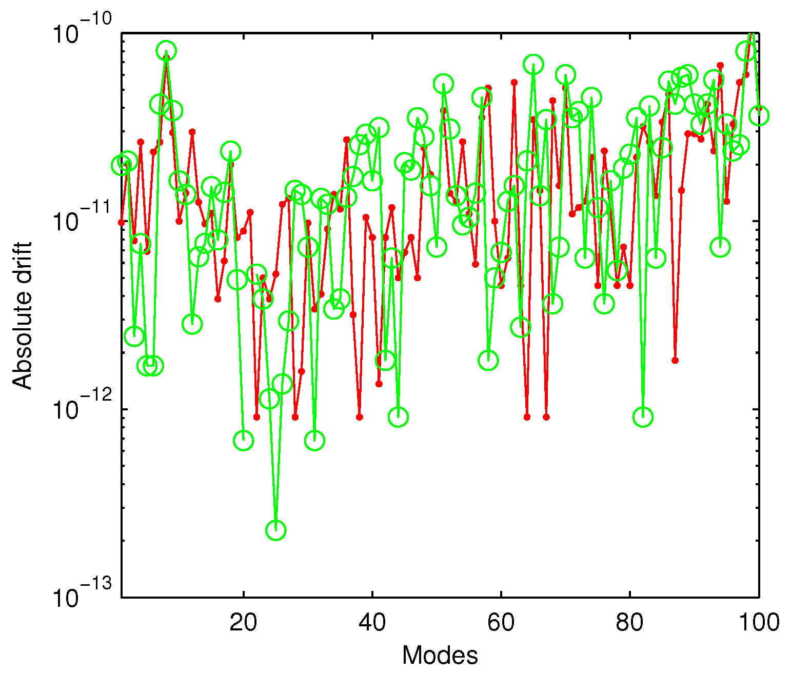
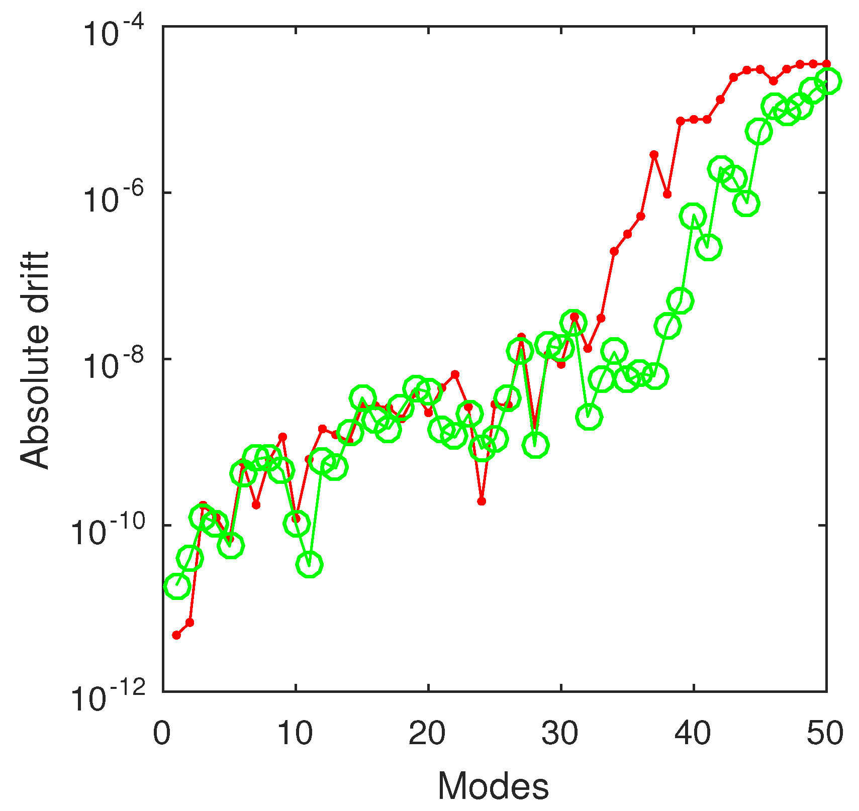
The absolute drift reported in Figure 1 means that we can compute the first hundred eigenvalues with better accuracy than . Unfortunately, no accuracy analysis is reported in [21,29,30].
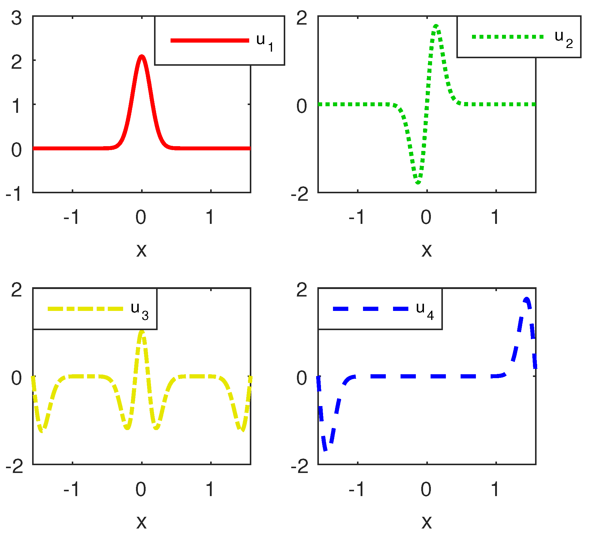
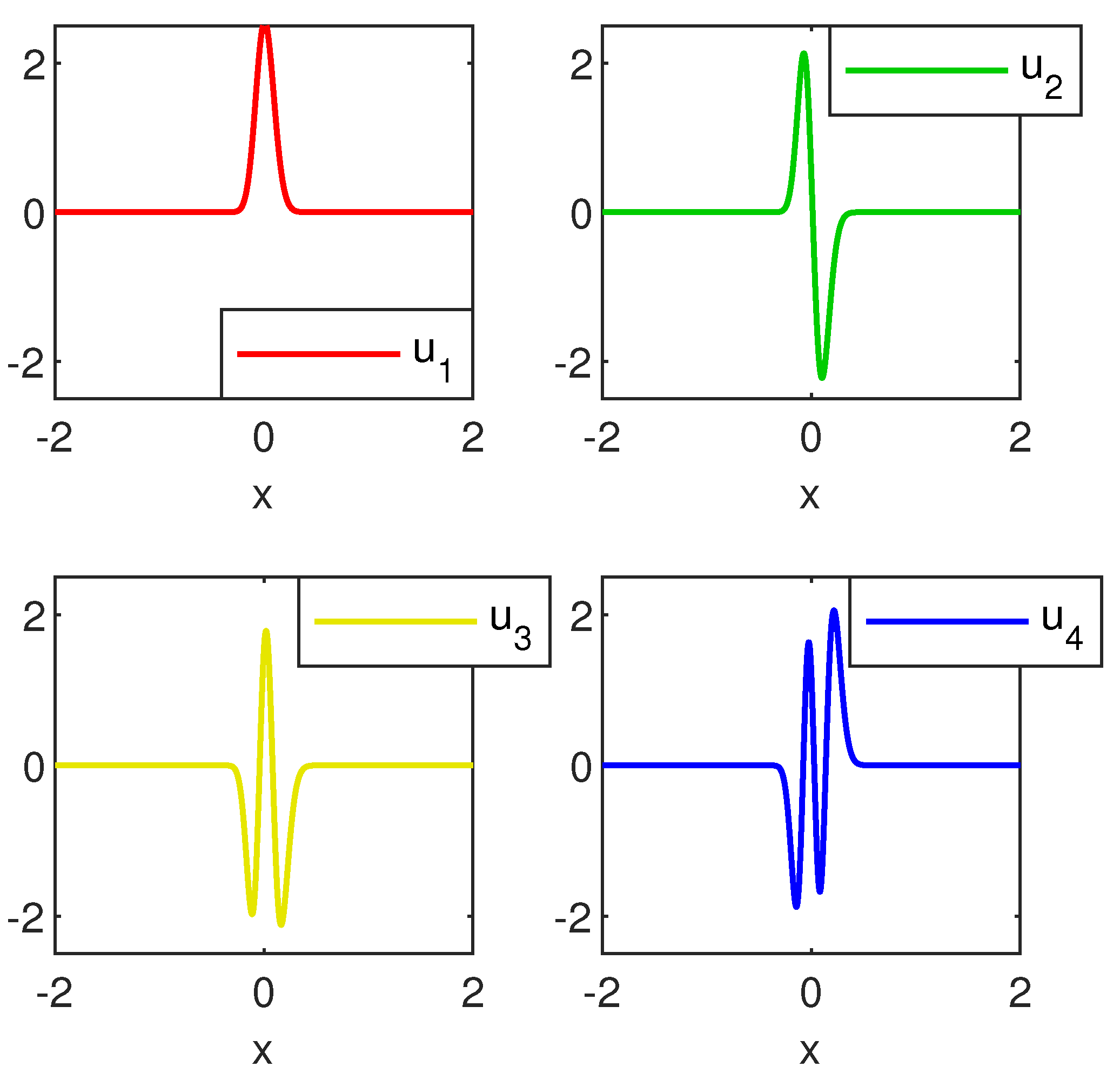
The eigenvectors are either symmetric (the even ones) or anti-symmetric (the odd ones). The first four of them are depicted in Figure 2. They look fairly smooth and satisfy the boundary conditions.
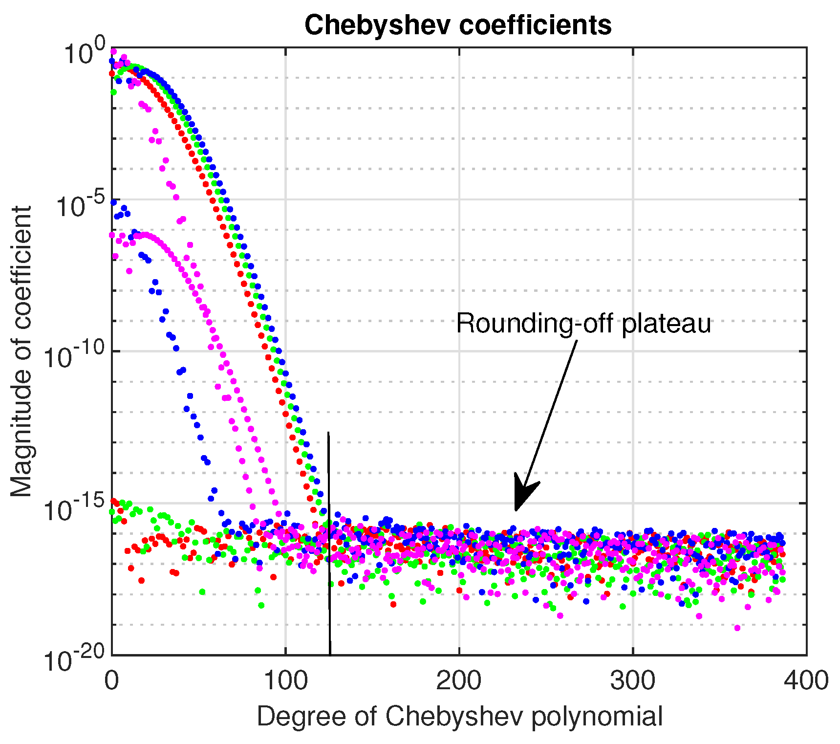
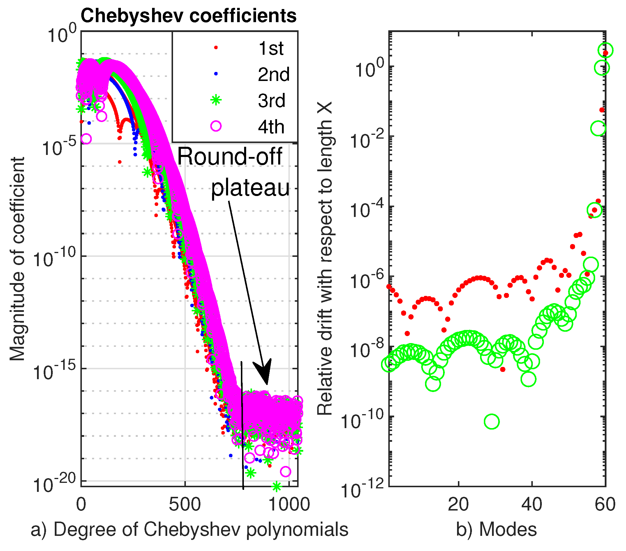
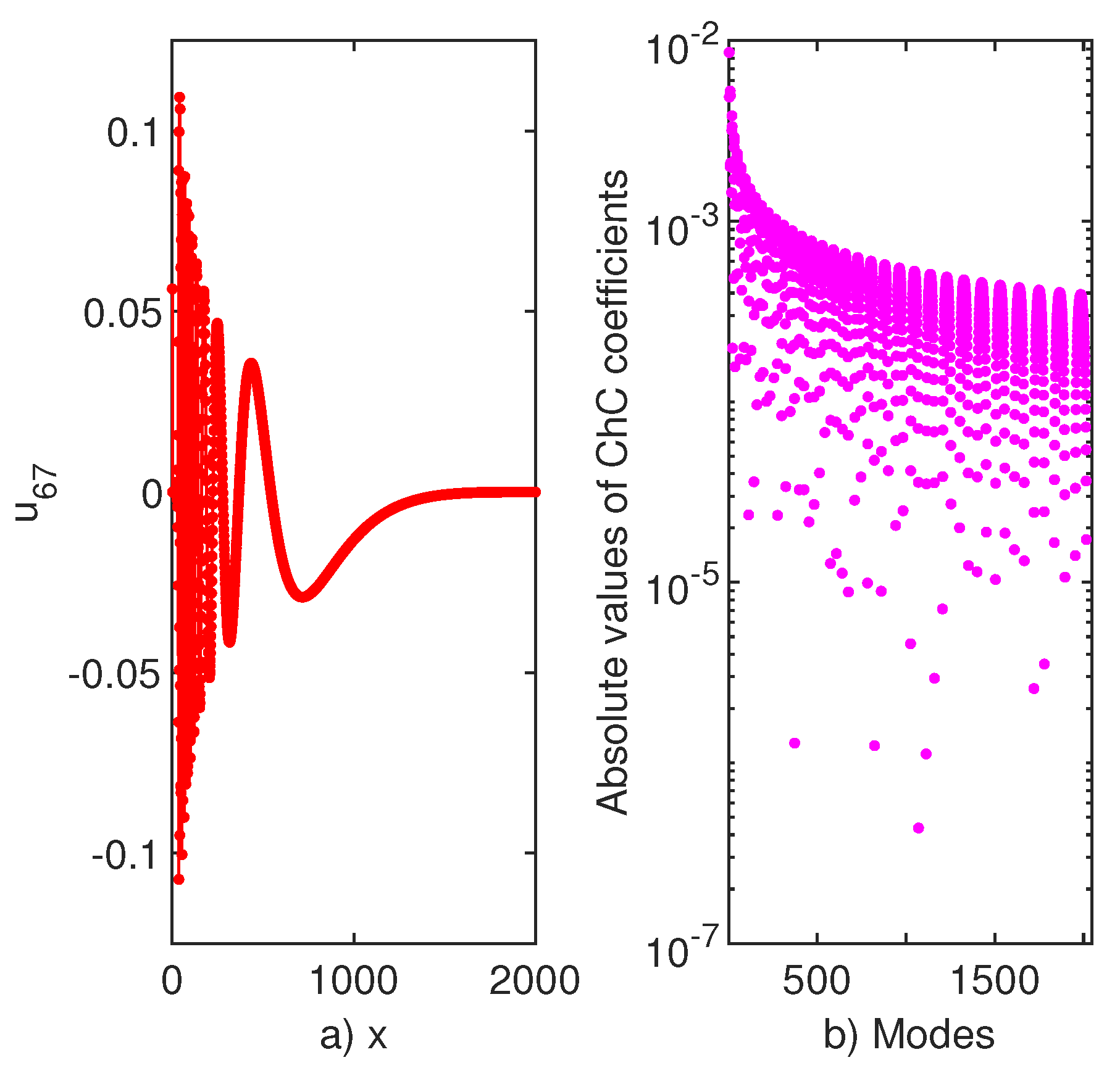
The Chebyshev coefficients of the first four eigenvectors of Coffey-Evans problem computed by Chebfun are displayed in Figure 3. These coefficients decrease sharply and smoothly to a rounding-off plateau below . Roughly speaking, this means they are computed with the machine precision.
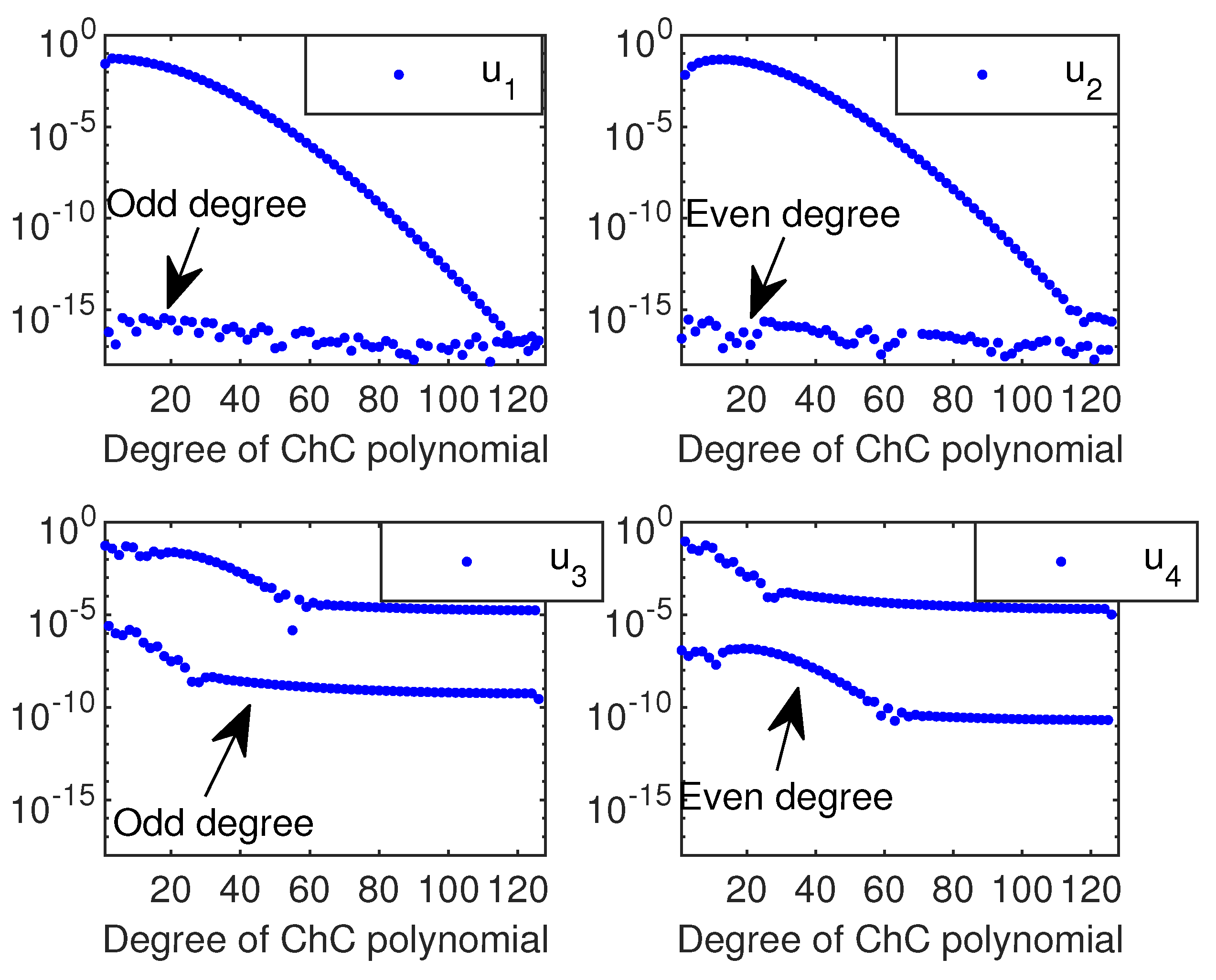
In order to obtain Figure 4, we have used the FCT (fast Chebyshev transform). It is very interesting to compare this figure with Figure 3. It becomes very clear that, except for the first two eigenvectors, ChC loses the accuracy with which it computes. Actually, by default, Chebfun tries to find the six eigenvalues whose eigenmodes are "most readily converged to", which approximately means the smoothest ones.
For this potential, the first eigenvalue is close to zero (actually we have got ) and there are very close eigenvalue triplets , , … as increases. The common numeric part of the eigenvalues in the first triplet is and that of the eigenvalues in the second is a little shorter, i.e.,
A selected set of eigenvalues computed by Chebfun and ChC are compared in Table 1 with those computed in [29]. An excellent agreement is visible.
The elapsed time used by Chebfun in finding the first 200 eigenvalues has equaled s. and ChC used for the same number of eigenvalues only s.
4.1.2. A Morse Potential with Deep Well
Let’s consider now Equation (1) with the potential
This problem is analyzed, among other works, in [17] where the author observes that the points are non oscillatory limit points according with Weyl’s classification. He does not indicate any boundary conditions for these points. However, from a physical point of view, the solutions must be bounded in these points (behavioral conditions). Our numerical experiments show that imposing homogeneous Dirichlet or Neumann boundary conditions practically obtains the same numerical results. Actually, we have used a Chebfun cod fairly analogue with that in the previous section. When we truncate the real axis to the interval with we get the following results:
i.e., eigenvalues which overlap to the sixth decimal on those reported in [17] (Problem 39).
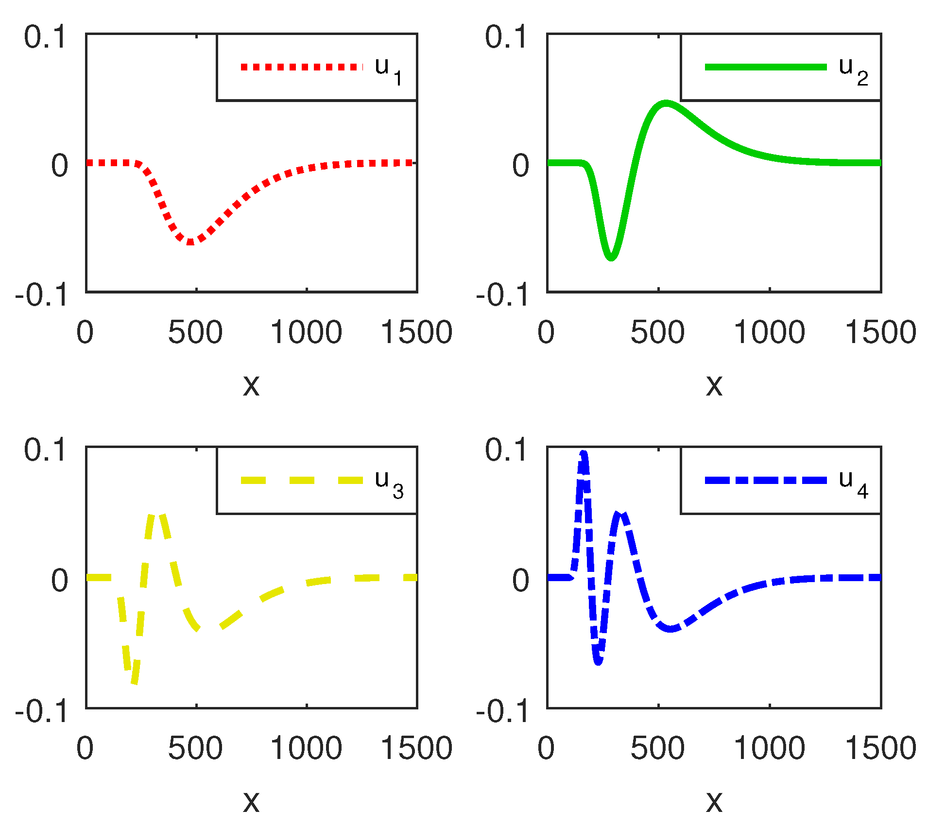
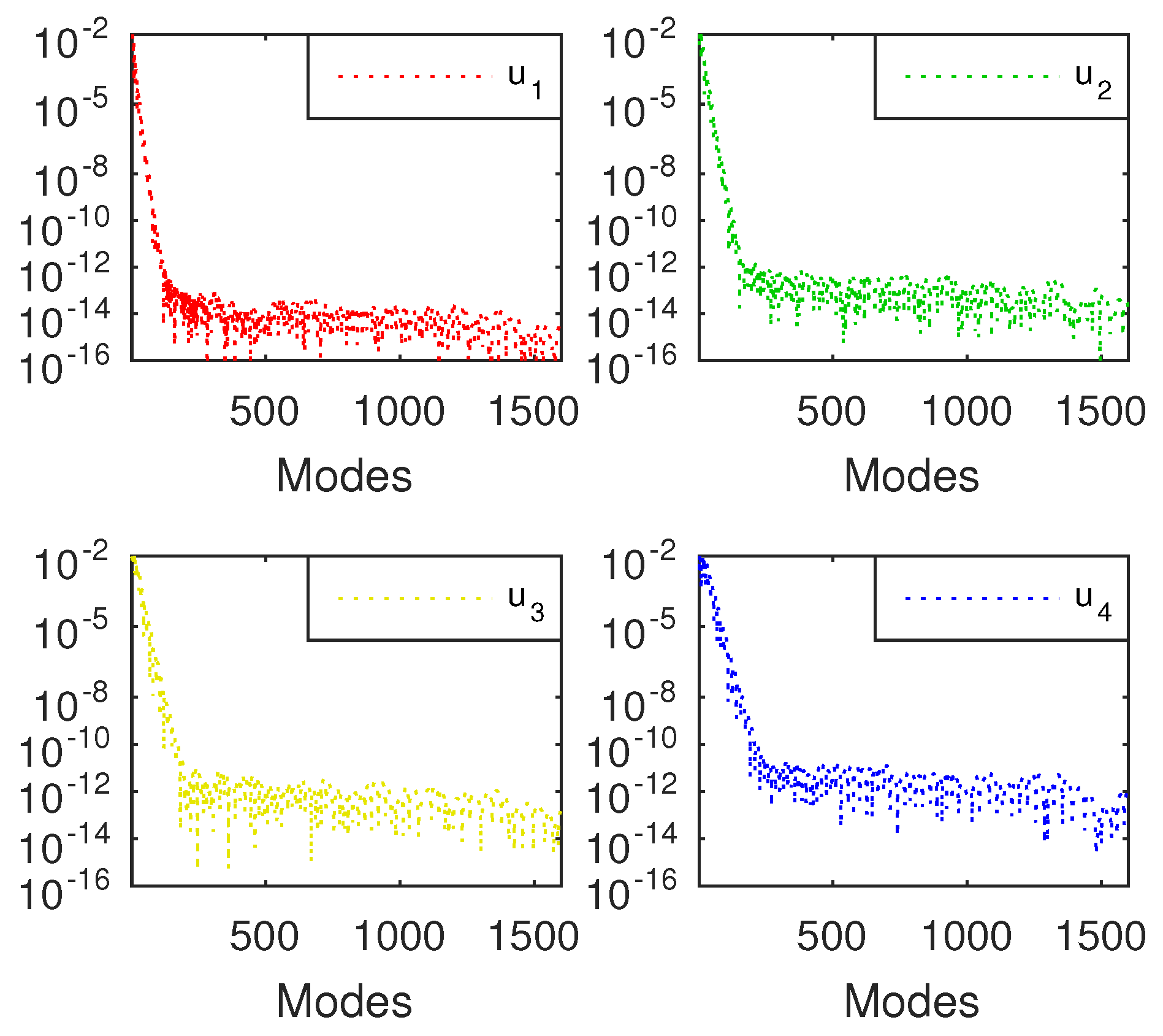
The first four eigenvectors are reported in Figure 5 and their coefficients are displayed in Figure 6a. They decrease smoothly, but Chebfun requires higher Chebyshev polynomials in order to resolve this problem than it required to solve the previous one. We can only put this fact on the considerably longer length of the integration interval.
In order to see how the accuracy of negative eigenvalues depends on the length of the computation interval X, in Figure 6b, we report the relative drift of these eigenvalues with respect to this parameter. It is visible that, in the second case, we can ensure an accuracy of order for most of these eigenvalues. Moreover, the computational process is numerically stable.
The elapsed time used by Chebfun in finding the first 200 eigenvalues has now equaled s.
It is important to note that, from the sixty eigenvalue on-wards, they become positive and closer as their indices increase. We consider this to be a reasonable approximation of the continuous part of the spectrum.
4.2. Two Half Range Singular Schrödinger Eigenproblems
In this section, we study the mixed spectrum of some Schrödinger eigenproblems having a “well dying out at infinity”potential.
4.2.1. Hydrogen Atom Equation
The first example consists of Equation (1) equipped with the potential
along with the boundary conditions
The problem (1), (5) and (6) is clearly singular in origin and is defined on an unbounded domain. We must mention from the beginning that our numerical experiments performed with LGRC and Chebfun together with the truncation of the domain did not produce satisfactory results. In these conditions, we have resorted to the mapped ChC method.
In order to implement this method, we use the algebraic map
which, for each c, transforms the interval into the half line, and its inverse. The scaling parameter c is free to be tuned for optimal accuracy.
The mapping (7) has been introduced in [31] where its practical effects have been discussed. The author observed that the convergence of the Chebyshev expansion is governed by the closeness of the singularities of the function being expanded to the expansion region. The major effect of such mapping is to allow us to move the singularities further away from the expansion region. The mapping may also weaken the effect of the singularities by modifying the strength of the singularity as well as moving it. The value of the scaling parameter c used in our computation was chosen essentially by trial and error along with the drift with respect to this parameter.
In order to write down any second order differential equation in independent variable s, we need the following derivatives:
Now, it is easy to write the differential equation for and to attach to this new equation the homogeneous Dirichlet boundary conditions As usual, we implement these conditions by deleting the first and the last rows and columns of the collocation matrix attached to the left-hand side of Equations (1)–(5). This is the most simplified version of removing technique of the independent boundary conditions introduced in [23]. With (8), the following MATLAB code solves this problem:
% approximation order and parameter l
N=1600; l=1;
% number of displayed eigenvalues
Ne=50;
c=2; % scaling factor
% Chebyshev differentiation matrices (Weideman & Reddy)
[st,D]=chebdif(N,2);
% N-2 kept nodes; 1 and N are removed nodes
k=2:N-1; s=st(k);
% enforced boundary conditions in differentiation matrices
D2=D(k,k,2); D1=D(k,k,1);
% collocation matrix of the system
A=-diag((1-x).^4)*D2/(4*(c^2))+diag((1-x).^3)*D1/(2*(c^2))+...
diag(l*(l+1)*((1-x).^2)./(((1+x).^2)*(c*2))-(1-x)./(c*(1+x)));
% computed and sorted eigenpairs
[U,S]=eig(A); S=diag(S); [t,o]=sort(S); S=S(o); U=U(:,o);
disp(S(1:Ne))
% Chebyshev coefficients of the first four eigenvectors by FCT
Ucoeff=fcgltran(U(:,1:4),1);
With respect to this code, we mention that we have introduced the boundary conditions in the mapped formulation by deleting the first and the last rows and columns in the differentiation matrices. It means that the first and the last nodes are removed as in the removing technique of independent boundary conditions introduced in [23].
The first four vectors of the problem are displayed in Figure 7. It is clear that they satisfy both boundary conditions, but, in the right neighborhood of origin, they have a totally different behavior from the eigenvectors of regular problems, i.e., they vanish out on continuous portions and not in discrete points. However, they clearly approximate square-integrable eigenfunctions and thus confirm some theoretical results proved in [12].
Their Chebyshev coefficients obtained using FCT (fast Chebyshev transform—see [32] for details) are displayed in Figure 8. They decrease sharply and smoothly to some limits, followed by a wide rounding-off plateau. For the first vector (the rightmost one), this limit is around . It increases with the index of the vector.
Roughly, this means that we cannot hope for a better approximation than something of the order when computing the first eigenvector.
When , mapped ChC has found , which is a very good approximation of The largest negative eigenvalue has been and the next eigenvalue, the smallest positive has been computed as In order to suggest how the mapped ChC method simulates the notion of continuous spectrum, we will provide in Table 2 some significant eigenvalues.
It is very important to note that the absolute drift with respect to N (including that to the exact eigenvalues) is of the order of , for the first two values, and increases to an order better than for the fifty eigenvalue (see Figure 9).
In the monograph [12] (Sect. 18), it is proved that, if the potential is continuous and has the asymptotic behavior as for , the spectrum is continuous and the eigenfunctions are not square-integrable and for the spectrum is discrete and the eigenfunctions are square-integrable. The numerical results gathered around this problem plainly confirm this analytical result.
Actually, the eigenvector corresponding to the first positive eigenvalue (the sixty-seventh one) is depicted in Figure 10a. It is hard to believe that this could approximate a square-integrable eigenfunction. In Figure 10b, we displayed the Chebyshev coefficients of the corresponding eigenvector. The oscillations of these coefficients mimic the steep oscillations of the eigenvector.
For the real scaling factor c, we have to mention that, in case of eigenvalue problems, it can be adjusted only on the mathematical basis. Thus, it can be tuned in order to:
- improve the decaying rate of the coefficients of spectral expansions.
- find as orthogonal as possible eigenvectors to an eigenproblem;
At the end of this section, we must mention that, even for a large order N, i.e., , the elapsed time did not exceed a few seconds. In fact, it reached s. It is also very important to emphasize that the existence of singularity forced us to work with such a high order of approximation in order to ensure a error in the computation of the first eigenvalues.
4.2.2. Potential with a Coulomb Type Decay
Let’s consider now the Schrödinger Equation (1) equipped with the singular potential (9)
and supplied with boundary conditions (6).
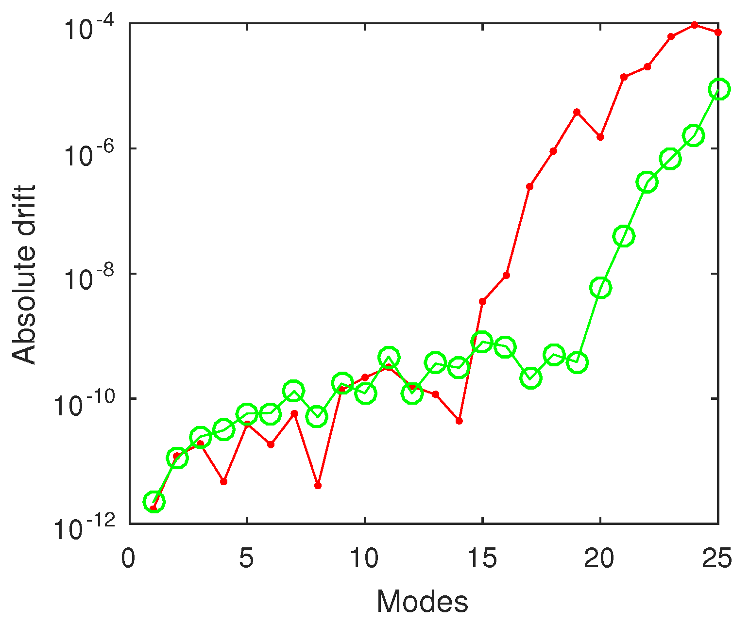
Some eigenvalues computed by the mapped ChC method when and are compared in Table 3 with their counterparts computed by LGRC and perturbation methods. If, for the first eigenvalues, the coincidence is excellent, the same does not happen for higher indices. This is why in Figure 11 in a log-linear plot we illustrate the absolute drift in the case of the ChC method. Consequently, we can firmly state that the eigenvalues calculated with ChC are the most correct. For example, the tenth eigenvalue is estimated with better accuracy than of the order . It is also clear from this figure that, in the second case, i.e., and , the drift oscillates less than in the first case reported.
4.3. A Singular Schrödinger Eigenproblem on the Real Line—the Anharmonic Oscillator
Let’s consider now the Equation (1) on the real line with the potential
where and are real parameters. This is a more general (anharmonic) oscillator than the simpler harmonic one.
Two behavioral boundary conditions requiring the boundedness of the solutions at large distance, i.e., are attached to this equation. Actually, we impose the conditions
We have to observe that these conditions are automatically satisfied in spectral collocation based on Laguerre, Hermite, and sinc functions.
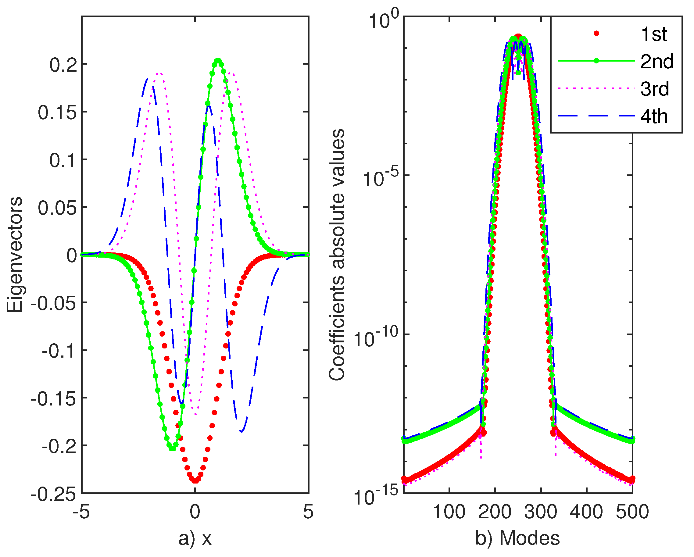
SiC with and scaling factor have been used in order to produce the following results. The fist four eigenvectors of Schrödinger eigenproblems (1)–(11) with potential (10) are displayed in Figure 12a. Their coefficients are illustrated in panel b of the same figure. These coefficients symmetrically decrease to approximations of at least which means a reasonable accuracy of the method.
We also have computed some high-lying eigenvalues namely , and , for and They have respectively the numerical values
They are five-digit approximation for the corresponding harmonic oscillator eigenvalues
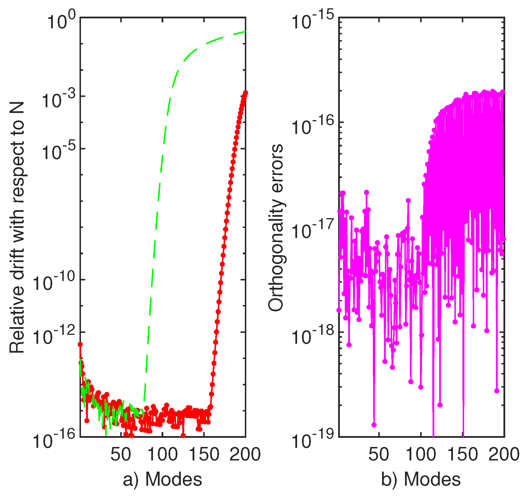
In [33], the author solved this problem numerically for general and . He used a very elegant variational argument of Ritz type, based on Hermite functions, and observed that, for large and fixed , the eigenvalues of this problem approximate those of the harmonic oscillator. We have confirmed this observation even for higher index eigenvalues. In the panel (a) of Figure 13, we display the relative drift of the first 200 eigenvalues of the problem. It is clear that approximately the first 70 eigenvalues are calculated with an accuracy better than . Eigenvalues with an index up to 150 remain at the same accuracy as Above this index, the accuracy decreases to .
Actually, over the years, a lot of literature has gathered on this problem. Low order eigenvalues have accurately computed, using Runge–Kutta type methods, for instance in [34,35]. In [36], the author used Hermite collocation in order to find only the first eigenvalues for some Schrödinger eigenproblem. With respect to the departure from orthogonality, i.e., the distance from zero of the scalar product of two eigenvectors, we display in panel b of Figure 13, in a log linear plot, the absolute values of the of the scalar products of and , It is again remarkable that this departure is less than i.e., close to the machine precision.
It is of some importance to justify our choice for SiC. Unlike all other methods of spectral collocation, where the differentiation matrices are highly non-normal, in SiC, these matrices are symmetric or skew-symmetric for even respectively odd values of cut-off parameter N. In addition, this is an important numerical advantage (see, for instance, our contribution [7]). For instance, in the MATLAB code below, we use the routine eigs instead of eig, which would have been more expensive and slower.
The following very simple MATLAB code has been used:
N=500; % order of approximation
h=0.1; % spacing (scaling factor)
[x,D]=sincdif(N,2,h); D2=D(:,:,2); % 2nd SiC differentiation
nu=1;mu=500; % parameter of the problem
A=-D2+diag((x.^2)+nu*(x.^2)./(1+mu*(x.^2)));% the matrix
[V,D] = eigs(A,250,0); D=diag(D); % call MATLAB code eigs
[t,o]=sort(real(D)); D=D(o); V=V(:,o); % sort eigenvalues
This code is fairly similar to that from Section 4.2.1 with two differences. First, the Chebyshev differentiation matrices are replaced by sinc differentiation matrices and then the boundary conditions are absent. More exactly, the discrete sinc functions, on which the unknown solution is expanded, are defined by
and satisfy the boundary conditions (11). In (12), the nodes are equidistant with spacing h and symmetric with respect to the origin.
The elapsed time required by SiC in order to solve this problem has equaled s.
4.4. The Sixth Order Hamiltonian
Let’s consider now the Equation (1) on the real line with the unbounded potential
supplied with the usual boundary conditions (11). This new problem is more challenging than the quartic oscillator. In this context, it is considered in [37] in a more general context. We have solved this problem by SiC as well as by Chebfun. In order to solve by SiC, we have used the MATLAB code from Section 4.3 and in the latter case we have used a MATLAB code similar to that from Section 4.1.1. Some selected eigenvalues are reported in Table 4.
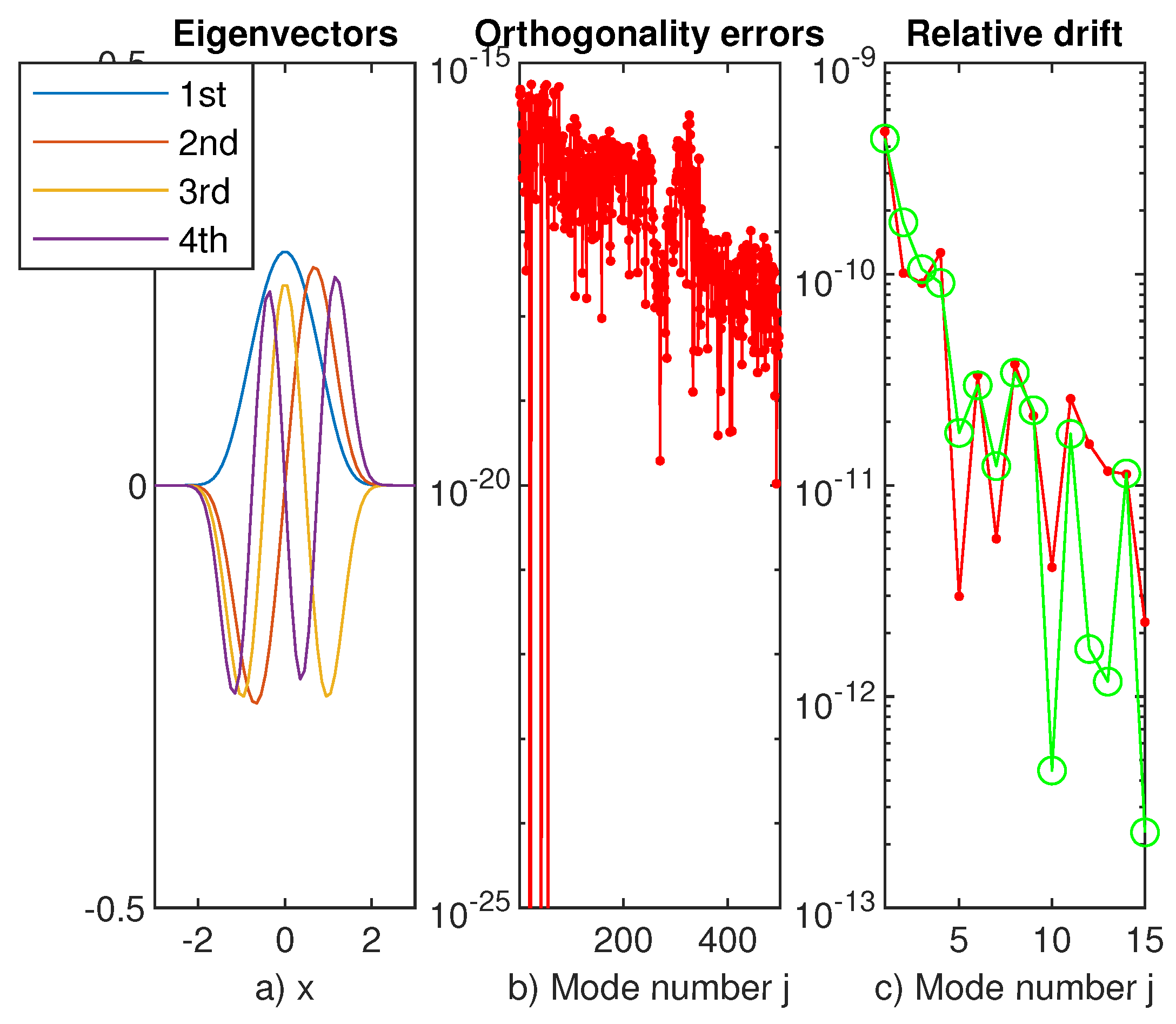
The first nine decimals coincide and the relative drift of the first fifteen eigenvalues, computed by SiC, is depicted in panel c of Figure 14. It justifies us to say that these eigenvalues are calculated with better accuracy than Panel b in the same figure shows that the first eigenvector is fairly orthogonal to the subsequent 499 of it. Actually, the first four eigenvectors are depicted in the first panel of Figure 14.
It is worth mentioning that, working with Chebfun, we have truncated the real axis to a finite symmetric interval . The computation of eigenvalues is stable with respect to the length The values reported in the second column of Table 4 have been computed with In this situation, the first four eigenvectors have been represented by Chebyshev polynomials of degree
The elapsed time in computing the first fifteen eigenvalues and all outcomes from Figure 14 by SiC equals s. The elapsed time working with Chebfun equals s. This means that the numerical process involved by Chebfun in choosing an optimal resolution is a little bit slower than a direct application of a spectral method with an apriori imposed resolution.
5. Concluding Remarks and Open Problems
A direct and global comparison between classical spectral methods and Chebfun in solving eigenvalue problems is almost impossible to conduct. We divided this into two stages.
First, for regular problems on finite domains, we have performed computations for various approximation orders N and then we have computed the relative or absolute drift of eigenvalues of interest. In this way, we have obtained these values with the desired accuracy. Typically, this accuracy is of the order of at least . Through the construction of Chebfun, this process is not applicable. In this case, the order of approximation is established automatically, but we are sure that the eigenvalues correspond to the smoothest eigenvectors, i.e., computed to the machine precision. The elapsed times have been of the order of a few seconds for ChC with a small plus for Chebfun.
For problems formulated on unbounded domains, on one hand, we have worked with mapped ChC or SiC. For both methods working with different approximation orders and then calculating the relative drift, we can ensure a certain accuracy. The elapsed time remains on the order of seconds or less. On the other hand, Chebfun can only work by truncating the domain in such a way that the singularity, at infinity or at the finite distance, is isolated.
As an absolute novelty, with respect to Chebfun, we have established the accuracy of the results by estimating the drift with respect to the length of the computation interval. In this way, we avoided the empirical truncation of the domain as is often the case. In our opinion, the way Chebfun operates in this situation is not fully established. However, in this case, the elapsed time can reach the order of some seconds.
Moreover, using the above mentioned absolute or relative drift, in terms of some parameters, we have ensured the numerical stability of the numerical process and can eliminate (numerically) spurious eigenvalues.
In other words, we have obtained automatically and precisely the accuracy at which a specified set of eigenvalues is computed.
However, approaching these problems whenever possible in parallel, with Chebfun as well as with the classical spectral methods, one can get greater confidence in the accuracy of numerical results.
The departure of orthogonality of a set of eigenvectors provides another useful hint for the accuracy of the numerical process.
In some examples, we have managed to correctly identify sets of multiple (triples) and high indices’ eigenvalues and even suggested the numerical meaning of the notion of continuous spectrum. This second issue obviously remains an open one.
All in all, we can say that Chebfun as well as classical spectral methods, in various forms, produce more accurate and comprehensive outcomes when solving singular as well as regular eigenproblems than classical non-spectral methods such as shooting, f. d., f. e. m., etc. In addition to the latter, both studied methods compute a large (as desired) set of eigenfunctions (eigenvectors) and give an indication of the accuracy of this calculation. However, there remains at least an open problem, namely that of establishing (possibly automatically) the scaling factor.
A final word of caution we think is appropriate. Unfortunately, we cannot offer an exact recipe on a method that must be applied for a particular problem. Only a careful approach with different methods can lead to the optimal method.
Funding
This research received no external funding.
Conflicts of Interest
The author declares no conflict of interest.
Abbreviations
The following abbreviations are used in this manuscript:
| c | scaling factor for unbounded domains |
| f. e. m. | finite element method |
| f. d. | finite difference method |
| GPS | generalized pseudospectral method |
| SL | Sturm–Liouville eigenproblem |
| ChC | Chebyshev collocation |
| LGRC | Laguerre–Gauss–Radau Collocation |
| SiC | sinc collocation |
| MATSLISE | Matlab package for SL and Schrödinger equations |
| MEP | multiparameter eigenvalue problem |
| N | the order of approximation of spectral method (cutting-off parameter) |
| SLEDGE | SL Estimates Determined by Global Errors |
| SLEIGN | FORTRAN package for numerical solution to SL eigenproblem |
| SLDRIVER | interactive package for the previous packages |
References
- Driscoll, T.A.; Bornemann, F.; Trefethen, L.N. The CHEBOP System for Automatic Solution of Differential Equations. BIT 2008, 48, 701–723. [Google Scholar] [CrossRef]
- Driscoll, T.A.; Hale, N.; Trefethen, L.N. Chebfun Guide; Pafnuty Publications: Oxford, UK, 2014. [Google Scholar]
- Driscoll, T.A.; Hale, N.; Trefethen, L.N. Chebfun-Numerical Computing with Functions. Available online: http://www.chebfun.org (accessed on 15 November 2019).
- Olver, S.; Townsend, A. A fast and well-conditioned spectral method. SIAM Rev. 2013, 55, 462–489. [Google Scholar] [CrossRef]
- Trefethen, L.N.; Birkisson, A.; Driscoll, T.A. Exploring ODEs; SIAM: Philadelphia, PA, USA, 2018. [Google Scholar]
- Trefethen, L.N. Approximation Theory and Approximation Practice; Extended Edition; SIAM: Philadelphia, PA, USA, 2019. [Google Scholar]
- Gheorghiu, C.I. Spectral Methods for Non-Standard Eigenvalue Problems. Fluid and Structural Mechanics and Beyond; Springer: Cham, Switzerland; Heidelberg, Germany; New York, NY, USA; Dordrecht, The Netherlands; London, UK, 2014. [Google Scholar]
- Gheorghiu, C.I. Spectral Collocation Solutions to Problems on Unbounded Domains; Casa Cărţii de Ştiinţă Publishing House: Cluj-Napoca, Romania, 2018. [Google Scholar]
- Weideman, J.A.C.; Reddy, S.C. A MATLAB Differentiation Matrix Suite. ACM Trans. Math. Softw. 2000, 26, 465–519. [Google Scholar] [CrossRef] [Green Version]
- Roy, A.K. The generalized pseudospectral approach to the bound states of the Hulthén and the Yukawa potentials. PRAMANA J. Phys. 2005, 65, 1–15. [Google Scholar] [CrossRef] [Green Version]
- Shizgal, B.D. Pseudospectral Solution of the Fokker–Planck Equation with Equilibrium Bistable States: The Eigenvalue Spectrum and the Approach to Equilibrium. J. Stat. Phys. 2016. [Google Scholar] [CrossRef]
- Birkhoff, G.; Rota, G.-C. Ordinary Differential Equations, 4th ed.; John Willey and Sons: New York, NY, USA, 1989; pp. 336–343. [Google Scholar]
- Cesarano, C.; Fornaro, C.; Vazquez, L. Operational results in bi-orthogonal Hermite functions. Acta Math. Univ. Comen. 2016, 85, 43–68. [Google Scholar]
- Cesarano, C. A Note on Bi-Orthogonal Polynomials and Functions. Fluids 2020, 5, 105. [Google Scholar] [CrossRef]
- Pruess, S.; Fulton, C.T. Mathematical Software for Sturm–Liouville Problem. ACM Trans. Math. Softw. 1993, 19, 360–376. [Google Scholar] [CrossRef]
- Pruess, S.; Fulton, C.T.; Xie, Y. An Asymptotic Numerical Method for a Class of Singular Sturm–Liouville Problems. SIAM J. Numer. Anal. 1995, 32, 1658–1676. [Google Scholar] [CrossRef]
- Pryce, J.D. A Test Package for Sturm–Liouville Solvers. ACM Trans. Math. Softw. 1999, 25, 21–57. [Google Scholar] [CrossRef]
- Pryce, J.D.; Marletta, M. A new multi-purpose software package for Schrödinger and Sturm–Liouville computations. Comput. Phys. Comm. 1991, 62, 42–54. [Google Scholar] [CrossRef]
- Bailey, P.B.; Everitt, W.N.; Zettl, A. Computing Eigenvalues of Singular Sturm–Liouville Problems. Results Math. 1991, 20, 391–423. [Google Scholar] [CrossRef] [Green Version]
- Bailey, P.B.; Garbow, B.; Kaper, H.; Zettl, A. Algorithm 700: A FORTRAN software package for Sturm–Liouville problems. ACM Trans. Math. Softw. 1991, 17, 500–501. [Google Scholar] [CrossRef]
- Ledoux, V.; Van Daele, M.; Vanden Berghe, G. MATSLISE: A MATLAB Package for the Numerical Solution of Sturm–Liouville and Schrödinger Equations. ACM Trans. Math. Softw. 2005, 31, 532–554. [Google Scholar] [CrossRef]
- Solomonoff, A.; Turkel, E. Global Properties of Pseudospectral Methods. J. Comput. Phys. 1989, 81, 230–276. [Google Scholar] [CrossRef]
- Hoepffner, J. Implementation of Boundary Conditions. Available online: http://www.lmm.jussieu.fr/hoepffner/boundarycondition.pdf (accessed on 25 August 2012).
- Gheorghiu, C.I.; Pop, I.S. A Modified Chebyshev-Tau Method for a Hydrodynamic Stability Problem. In Proceedings of the International Conference on Approximation and Optimization (Romania)—ICAOR, Cluj-Napoca, Romania, 29 July–1 August 1996; Volume II, pp. 119–126. [Google Scholar]
- Gheorghiu, C.I. On the numerical treatment of the eigenparameter dependent boundary conditions. Numer. Algor. 2018, 77, 77–93. [Google Scholar] [CrossRef]
- Gheorghiu, C.I.; Hochstenbach, M.E.; Plestenjak, B.; Rommes, J. Spectral collocation solutions to multiparameter Mathieu’s system. Appl. Math. Comput. 2012, 218, 11990–12000. [Google Scholar] [CrossRef] [Green Version]
- Plestenjak, B.; Gheorghiu, C.I.; Hochstenbach, M.E. Spectral collocation for multiparameter eigenvalue problems arising from separable boundary value problems. J. Comput. Phys. 2015, 298, 585–601. [Google Scholar] [CrossRef] [Green Version]
- Boyd, J.P. Traps and Snares in Eigenvalue Calculations with Application to Pseudospectral Computations of Ocean Tides in a Basin Bounded by Meridians. J. Comput. Phys. 1996, 126, 11–20. [Google Scholar] [CrossRef]
- Ledoux, V.; Van Daele, M.; Vanden Berghe, G. Efficient computation of high index Sturm–Liouville eigenvalues for problems in physics. Comput. Phys. Commun. 2009, 180, 241–250. [Google Scholar] [CrossRef] [Green Version]
- Ledoux, V.; Ixaru, L.Gr.; Rizea, M.; Van Daele, M.; Vanden Berghe, G. Solution of the Schrödinger equation over an infinite integration interval by perturbation methods, revisited. Comput. Phys. Commun. 2006, 175, 612–619. [Google Scholar] [CrossRef]
- Schonfelder, J.L. Chebyshev Expansions for the Error and Related Functions. Math. Comput. 1978, 32, 1232–1240. [Google Scholar] [CrossRef]
- Von Winckel, G. Fast Chebyshev Transform (1D). Available online: https://www.mathworks.com/matlabcentral/fileexchange/4591-fast-chebyshev-transform-1d (accessed on 15 May 2015).
- Mitra, A.K. On the interaction of the type . J. Math. Phys. 1978, 19, 2018–2022. [Google Scholar] [CrossRef]
- Simos, T.E. Some embedded modified Runge–Kutta methods for the numerical solution of some specific Schrödinger equations. J. Math. Chem. 1998, 24, 23–37. [Google Scholar] [CrossRef]
- Simos, T.E. An accurate finite difference method for the numerical solution of the Schrödinger equation. J. Comput Appl. Math. 1998, 91, 47–61. [Google Scholar] [CrossRef] [Green Version]
- Trif, D. Matlab package for the Schrödinger equation. J. Math. Chem. 2008, 43, 1163–1176. [Google Scholar] [CrossRef]
- Szalay, V.; Czakó, G.; Nagy, A.; Furtenbacher, T.; Császár, A.G. On one-dimensional discrete variable representations with general basis functions. J. Chem. Phys. 2003, 119, 10512–10518. [Google Scholar] [CrossRef] [Green Version]
Figure 1.
The drift of the first 100 eigenvalues of the Coffey-Evans problem. ChC used the orders of approximations and -red dotted line and, respectively, and -green circled line.
Figure 1.
The drift of the first 100 eigenvalues of the Coffey-Evans problem. ChC used the orders of approximations and -red dotted line and, respectively, and -green circled line.

Figure 2.
The first four eigenvectors of the Coffey-Evans problem computed by Chebfun.

Figure 3.
In a log-linear plot, the Chebyshev coefficients of the first four eigenvectors of the Coffey-Evans problem computed by Chebfun.
Figure 3.
In a log-linear plot, the Chebyshev coefficients of the first four eigenvectors of the Coffey-Evans problem computed by Chebfun.

Figure 4.
In a log-linear plot, the Chebyshev coefficients of the first four eigenvectors of the Coffey-Evans problem computed by ChC.
Figure 4.
In a log-linear plot, the Chebyshev coefficients of the first four eigenvectors of the Coffey-Evans problem computed by ChC.


Figure 6.
(a) In a log-linear plot, the Chebyshev coefficients of the first four eigenvectors of problem (1) equipped with the Morse potential (4). (b) The relative drift of the negative eigenvalues of this problem with respect to the length of the interval of integration red dots correspond to and , and the green circles correspond to and to .

Figure 7.
The first four eigenvectors for the hydrogen atom eigenproblems (1), (5), and (6) with computed by mapped ChC with scaling factor and

Figure 8.
The coefficients of the first four eigenvectors for hydrogen atom eigenproblems (1), (5), and (6) with computed by mapped ChC with scaling factor and

Figure 9.
The absolute drift with respect to N of the first 50 negative eigenvalues of the hydrogen atom eigenproblems (1), (5), and (6) computed by mapped ChC with scaling factor and and (red line). The green circled line signifies the drift of eigenvalues computed by mapped ChC using with respect to the exact eigenvalues corresponding to

Figure 10.
(a) The eigenvector corresponding to the first positive eigenvalue of hydrogen atom eigenproblems (1), (5), and (6) computed by mapped ChC with scaling factor and , (left panel). (b) In the right panel, in a log-linear plot, we display the Chebyshev coefficients of this eigenvector.

Figure 11.
The absolute drift with respect to N of the first 25 eigenvalues for the Schrödinger problems (1)–(6) with Coulomb-type decay potential (9), computed by mapped ChC with scaling factor ; red dotted line for the case and and green circled line for the case and

Figure 12.
(a) Zoom in the first four eigenvectors computed by SiC for the Schrödinger eigenproblems (1)–(11) with potential (10). (b) The sinc coefficients for these vectors. We mention that the figure in panel (a) has the same legend as that in panel (b).

Figure 13.
(a) The relative drift of the first 200 eigenvalues of problems (1)–(11) with potential (10), and -red dotted line and and -green line. (b) In the right panel, we display the orthogonality errors (deficiency) of the first eigenvector of the same problem with respect to the subsequent 199 of it.

Figure 14.
(a) The first four eigenvectors of problem (13) computed with and scaling factor ; (b) the orthogonality errors (deficiency) of the first eigenvector of the same problem with respect to the subsequent 499 of it; (c) the relative drift of the first 15 eigenvalues of problem (13) and -red dotted line and and -green line.


Table 1.
High index eigenvalues of Schrödinger eigenproblem equipped with Coffey-Evans potential (3) computed by three different methods.
Table 1.
High index eigenvalues of Schrödinger eigenproblem equipped with Coffey-Evans potential (3) computed by three different methods.
| by Chebfun | According to [29] | by ChC | |
|---|---|---|---|
| 10,653.52543568510 | 10,653.525435875921 | 10,653.52543587600 | |
| 40,851.63764596094 | 40,851.637646050455 | 40,851.63764605047 |
Table 3.
The first five eigenvalues and the tenth one of the Schrödinger problem (1)–(6) when the potential has a Coulomb-type decay (9), computed by three different methods.
| Computed by LGRC in [8] | According to [30] | by Mapped ChC | |
|---|---|---|---|
Table 4.
Some eigenvalues of the Schrödinger problem (13) computed by three different methods.
Publisher’s Note: MDPI stays neutral with regard to jurisdictional claims in published maps and institutional affiliations. |
© 2020 by the author. Licensee MDPI, Basel, Switzerland. This article is an open access article distributed under the terms and conditions of the Creative Commons Attribution (CC BY) license (http://creativecommons.org/licenses/by/4.0/).
Share and Cite
MDPI and ACS Style
Gheorghiu, C.-I. Accurate Spectral Collocation Computation of High Order Eigenvalues for Singular Schrödinger Equations. Computation 2021, 9, 2. https://0-doi-org.brum.beds.ac.uk/10.3390/computation9010002
AMA Style
Gheorghiu C-I. Accurate Spectral Collocation Computation of High Order Eigenvalues for Singular Schrödinger Equations. Computation. 2021; 9(1):2. https://0-doi-org.brum.beds.ac.uk/10.3390/computation9010002
Chicago/Turabian StyleGheorghiu, Călin-Ioan. 2021. "Accurate Spectral Collocation Computation of High Order Eigenvalues for Singular Schrödinger Equations" Computation 9, no. 1: 2. https://0-doi-org.brum.beds.ac.uk/10.3390/computation9010002
Note that from the first issue of 2016, this journal uses article numbers instead of page numbers. See further details here.