Finite Element Simulation of Thermo-Mechanical Model with Phase Change

Abstract

In this work, we consider a mathematical model and finite element implementation of heat transfer and mechanics of soils with phase change. We present the construction of the simplified mathematical model based on the definition of water and ice fraction volumes as functions of temperature. In the presented mathematical model, the soil deformations occur due to the porosity growth followed by the difference between ice and water density. We consider a finite element discretization of the presented thermoelastic model with implicit time approximation. Implementation of the presented basic mathematical model is performed using FEniCS finite element library and openly available to download. The results of the numerical investigation are presented for the two-dimensional and three-dimensional model problems for two test cases in three different geometries. We consider algorithms with linearization from the previous time layer (one Picard iteration) and the Picard iterative method. Computational time is presented with the total number of nonlinear iterations. A numerical investigation with results of the convergence of the nonlinear iteration is presented for different time step sizes, where we calculate relative errors for temperature and displacements between current solution and reference solution with the largest number of the time layers. Numerical results illustrate the influence of the porosity change due to the phase-change of pore water into ice on the deformation of the soils. We observed a good numerical convergence of the presented implementation with the small number of nonlinear iterations, that depends on time step size.

1. Introduction

Permafrost covers almost a quarter of the land area in the Northern Hemisphere. Many people around the world live in permafrost and seasonal frozen areas in Alaska, Canada, and Russia (Na and Sun [1], Yu et al. [2], Tounsi et al. [3], Marchenko et al. [4], Knoblauch et al. [5]). The ground freezing and thawing process can change the shape of the land surface and damage constructions and buildings in the permafrost area (Zhou and Meschke [6], Sweidan et al. [7], Xu et al. [8]). Moreover, buildings constructed in the permafrost area can create heat that thaws the underlying grounds. Thawed soil becomes soft and uneven and can destroy houses and buildings. In order to prevent ground warming, buildings are constructed on pile foundations (Shang et al. [9], Nixon [10], Foriero and Ladanyi [11]). Construction of roads, bridges, railways, and other types of transport infrastructure is also a major problem in the permafrost zone as soil thawing damages them and requires constant repairs to keep them safe. Moreover, the overall rise in annual temperatures and releasing greenhouse gases into the atmosphere lead to further climate change on a global level. The global climate is getting warmer and making the frozen ground thaw (Nixon [10], Buteau et al. [12], Delisle [13]). Permafrost contains deposits of carbon matter, and global climate warming can release carbon dioxide and methane into the atmosphere (Knoblauch et al. [5], Stepanenko et al. [14], Khvorostyanov et al. [15]). Permafrost thawing can also release ancient bacteria and viruses that were frozen and inactive before (Jansson and Taş [16]). Unfrozen bacteria can cause severe diseases dangerous for humans and animals. Thawing permafrost may have a dramatic impact on our planet and its residents. Therefore, it is necessary to build appropriate mathematical models for numerical simulation of the ongoing processes in order to understand them and fight the problem (Li et al. [17], Neaupane and Yamabe [18], Nishimura et al. [19]).

Frost heaves and soil thawing are complex processes involving heat transfer and deformations, as well as pore water flow processes. Multiphysical mathematical models are usually used to describe complex interactions between thermal, hydraulic, and mechanical fields (THM). Li et al. [17] presented a thermal-hydraulic-mechanical model with water-ice phase change. The model was developed by combining a heat transfer model with ice-water phase change and the THM model via a simplified algorithm. Implementation was based on the FLAC3D software package, where the water-ice phase transition was implemented as an extension. Coupling to the displacements field was done without consideration of the porosity change due to water-ice phase transition and only contained part related to the linear thermal expansion coefficient of the solid matrix. The coupled thermo-hydro-mechanical process in rock mass under freezing/thawing condition was studied by Kang et al. [20], where the relation between the freezing point and pore pressure was derived from taking into account volume expansion of water during the freezing process. The simulation of the THM model was performed using finite difference approximation and implemented based on FLAC3D software. Na and Sun [1] presented the stabilized thermo-hydro-mechanical model with the elasto-plastic responses and influence of phase transitions, where the influence of the phase-change processes was done by a pressure change with complicated relationships for elasto-plastic effects. In order to solve the highly nonlinear thermo-hydro-mechanical model, the finite element approximation with stabilization was used to handle the lack of inf–sup condition. The highly nonlinear coupled discrete system was solved using the block-preconditioned Newton–Krylov solvers, where implementation was based on the deal.II library (Bangerth et al. [21]). A fully coupled thermo-hydro-mechanical finite element model was formulated by Nishimura et al. [19]. The elasto-plastic mechanical model was used to adopt total stress, liquid pressure, and ice pressure. The performance of the model was tested for the important cold region infrastructure topic of frost heaving. Neaupane et al. [22] described a nonlinear elasto-plastic simulation of freezing and thawing of rock. Numerical modeling was performed using the finite element method and the Newton–Raphson method to solve the nonlinear equations. A theoretical formulation of the non-isothermal flow and deformation model in unsaturated porous media was presented by Khalili and Loret [23]. The model describes thermo-hydro-mechanical coupling processes and takes into account phase exchange (vaporization, condensation), and considers an elasto-plastic behavior. Exadaktylos [24] presented the formulation of the freezing/thawing model for saturated porous media and considered numerical implementation for one-dimensional formulation using the finite element method. However, most real-life applications are two or three-dimensional. Formulation of the model and finite difference scheme of heat and water flow during soil freezing was presented by Taylor and Luthin [25]. Zhou and Li [26] established a coupled mathematical model of water, heat, and stress with the relationship between effective stress and void ratio, Clapeyron equation, and the relationship between the content of unfrozen water and temperature. The presented mathematical model was implemented using COMSOL software for a one-dimensional example. Implementation of the three-phase thermo-hydro-mechanical finite element model for freezing soils was presented by Zhou and Meschke [6]. The implementation was based on the finite-element code KRATOS (Dadvand et al. [27]). Numerical results were given for one-dimensional Terzaghi’s consolidation problem and soil freezing problem during tunneling. The different formulation of the frost heave model was presented by Michalowski and Zhu [28], where the concept of porosity rate function was given. Zhang and Michalowski [29,30] developed an elastic-plastic constitutive model to simulate the freezing and thawing of soils. The mathematical model describes a frost heaving using the porosity rate function, which simulates the growth of ice lenses as average growth in porosity. The model was implemented in the commercial finite-element system ABAQUS.

Simulations of the applied problems require the construction of complex domains. In order to numerically solve a mathematical model, unstructured computational meshes should be constructed to the accurate approximation of the problem in geometrically complex domains. The common approach used for approximation of multiphysical problem on an unstructured grid is the finite element method (Brenner and Scott [31], Hughes [32]). In our previous works (Pavlova et al. [33], Vabishchevich et al. [34]), we considered the heat transfer problem with phase change and presented finite element approximation on unstructured grids for complex geometries (Pavlova et al. [33], Vabishchevich et al. [34]). The results of simulations for several applied problems in three-dimensional formulations illustrated the applicability of the method. For numerical implementation, we used an open-source finite-element library FEniCS (Logg et al. [35]). In FEniCS, we used a PETSc based solver to solve a large system of equations on high-performance computing systems (Balay et al. [36]). The PETSc library is a leading software framework for parallel scientific computing. In (Kolesov et al. [37]), we presented an implementation of the poroelasticity model using the PETSc library, where splitting schemes were constructed and investigated for multidimensional test problems on high-performance systems with distributed memory. Recently, we considered the construction of the mixed dimensional mathematical model for artificial freezing problems in permafrost area in (Vasilyeva et al. [38]), where we presented a multiscale method with additional multiscale basis functions for the solution of the Stefan problem in heterogeneous media for two and three-dimensional formulations. In this work, we continue the development of mathematical models with finite element approximation for problems in permafrost.

In this work, we consider a basic thermoelastic model that takes into account the deformations of porous media due to the phase change of pore water to ice. We start with the description of a thermo-mechanical model of soils with phase-change. The mathematical model is based on a definition of water fraction volume as a function of temperature using the relationship for unfrozen water content. In (Tice et al. [39], Michalowski [40]), the estimation of unfrozen water content function based on experimental tests is given, where parameters of the model depend on soil type and, in general, are different for freezing and thawing processes. Using mass conservation of frozen and thawed water, we describe ice volume fraction. As the sum of ice and unfrozen water fraction equals porosity, we can define a relationship for porosity as a function of temperature. Soil deformations occur due to porosity growth caused by the difference in ice and water density. The presented mathematical model is described by a nonlinear system of equations for temperature and displacements. The novelty of the paper is related to (1) derivation of the simplified mathematical model that takes into account porous water/ice phase-change and its influence on the mechanical deformations of soils; (2) construction and implementation of finite element approximation in order to numerically investigate model with an implicit scheme for approximation by time and Picard iterations for nonlinear coefficients for two and three-dimensional formulations. Implementation of the presented basic mathematical model is performed using FEniCS finite element software (Logg et al. [35]). The code is written using C++ Programming Language to perform fast calculations of multidimensional problems. We present numerical results for model problems in two- and three-dimensional formulations for two test cases in three different geometries. A numerical investigation is presented for different time step sizes, where we calculate relative errors for temperature and displacements. We consider algorithms with linearization from the previous time layer (one Picard iteration) and the Picard iterative method. Numerical results are presented with the number of nonlinear iterations. Finally, we discuss the computational time of the presented implementation with linearization from the previous time layer and the Picard iterative method. For the numerical solution of the arisen linear system of equations, we use a direct solver for both temperature and displacements fields. In future works, we will consider the numerical solution of the complex thermoelasticity model with phase-change on high-performance computing systems. The more complex models will be considered in future works by adding elastoplastic effects, the effect of the fluid flow, and ice lens formations.

The paper is organized as follows. In Section 2, we describe the basic concepts used in the construction of the mathematical model. In Section 3, we describe heat transfer processes in porous media and consider the mechanics of soils due to phase-change of the pore water into ice. For the numerical solution of the thermo-mechanical model, we present a finite element approximation in Section 4. Numerical results for model problems are presented in Section 5 for two- and three-dimensional formulations. The paper ends with conclusions.

2. Preliminaries

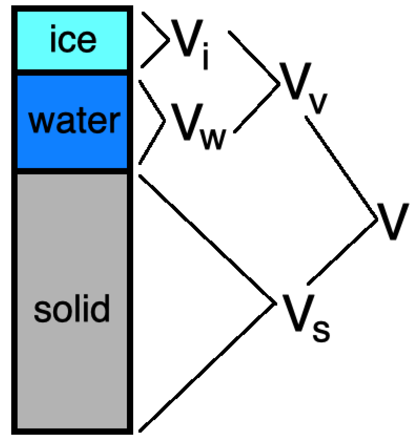
Let $V_w$, $V_i$, and $V_s$ be water, ice, and solid volumes of porous media, and

$$V_w+V_i=V_v,V_v+V_s=V,$$

where V is a total volume, and $V_v$ is a volume of void space that is filled with water or/and ice. The volume representation is shown in Figure 1 (Zhang [30]).

Let ${\Theta }_w$, ${\Theta }_i$, and ${\Theta }_s$ be water, ice, and solid fraction volumes

$${\Theta }_w=\frac{V_w}{V},{\Theta }_i=\frac{V_i}{V},{\Theta }_s=\frac{V_s}{V}$$

and

$${\Theta }_w+{\Theta }_i+{\Theta }_s=1,$$

where superscripts s, w, and i denote solid, unfrozen water and ice, respectively.

The porosity is defined as follows

$$\varphi =\frac{V_v}{V}$$

and therefore

$${\Theta }_i+{\Theta }_w=\varphi {\Theta }_s=(1-\varphi ).$$

We define unfrozen water content as follows

$$w=\frac{{\rho }_w{V}_w}{{\rho }_s{V}_s},$$

where ${\rho }_w$ and ${\rho }_s$ are density of water and solid, respectively. Note that the unfrozen water content function parameters depend on soil type and, in general, are different for freezing and thawing processes. The following model is used in (Tice et al. [39], Michalowski [40])

$$w\left(T\right)=\left\{\begin{array}{cc}\overline{w},\hfill & T\ge T_f,\hfill \\ w^{*}+(\overline{w}-w^{*})exp\left(a\right[T-T_f\left]\right),\hfill & T<T_f,\hfill \end{array}\right.$$

(1)

where T is a given temperature, $T_f$ is a freezing temperature and a is a model parameter ${[}^{°}{\mathrm{C}}^{-1}]$, $\overline{w}$ and $w^{*}$ are maximum and minimum water contents.

Therefore, using w, we have

$${\Theta }_w=\frac{V_w}{V}=\left(\frac{{\rho }_w{V}_w}{{\rho }_s{V}_s}\right)\frac{{\rho }_s}{{\rho }_w}\frac{V_s}{V}=w\frac{{\rho }_s}{{\rho }_w}(1-\varphi ).$$

In order to find a relationship that determines porosity changes due to water freezing or thawing processes, mass conservation of water in frozen and thawed phases is used

$${\rho }_w{\overline{V}}_w={\rho }_w{V}_w+{\rho }_i{V}_i,$$

where ${\rho }_i$ is an ice density and ${\overline{V}}_w$ is a water volume for $T\ge T_f$.

Therefore

$$\overline{w}=w+\frac{{\rho }_i{V}_i}{{\rho }_s{V}_s},$$

and

$${\Theta }_i=\frac{V_i}{V}=\left(\frac{{\rho }_i{V}_i}{{\rho }_s{V}_s}\right)\frac{{\rho }_s}{{\rho }_i}\frac{V_s}{V}=(\overline{w}-w)\frac{{\rho }_s}{{\rho }_i}(1-\varphi ).$$

Next, we can find a relationship for porosity

$$\varphi ={\Theta }_w+{\Theta }_i=(1-\varphi )\left[w\frac{{\rho }_s}{{\rho }_w}+(\overline{w}-w)\frac{{\rho }_s}{{\rho }_i}\right]$$

and

$$\varphi =\frac{w\frac{{\rho }_s}{{\rho }_w}+(\overline{w}-w)\frac{{\rho }_s}{{\rho }_i}}{1+w\frac{{\rho }_s}{{\rho }_w}+(\overline{w}-w)\frac{{\rho }_s}{{\rho }_i}}.$$

An obtained relationship for porosity, water, and ice fraction volumes will be used in the thermo-mechanical model.

3. Mathematical Model

In this section, we present a thermo-mechanical mathematical model for the simulation of heat transfer and mechanics in soils. We start with the equation for heat transfer in porous media. Then, we describe the mechanical model. Finally, we present the thermo-mechanical problem formulation.

3.1. Heat Transfer in Porous Media

The heat transfer in porous media is based on the energy conservation principle that can be written as follows (Michalowski and Zhu [28], Michalowski [40])

$$c\rho \frac{\partial T}{\partial t}-L{\rho }_i\frac{\partial {\Theta }_i}{\partial t}-\nabla ·(k\nabla T)=0,$$

(2)

where T is a temperature, L is the latent heat of fusion of water per unit mass, k is a heat conductivity, and c is a specific heat capacity, and $\rho$ is a density.

By mixture theory for saturated soils, we have

$$\begin{array}{cc}\hfill c\rho & ={\Theta }_s{c}_s{\rho }_s+{\Theta }_i{c}_i{\rho }_i+{\Theta }_w{c}_w{\rho }_w,\hfill \end{array}$$

(3)

where $c_j$ and ${\rho }_j$ are heat capacities (per unit mass) and densities for water, ice, and solid ($j=w,i,s$).

Heat conductivity can be calculated using the following model (Michalowski and Zhu [28])

$$k=k_s^{{\Theta }_s}{k}_i^{{\Theta }_i}{k}_w^{{\Theta }_w},$$

(4)

where $k_w$, $k_i$ and $k_s$ are water, ice and solid heat conductivities.

For water, ice, and solid fraction volumes and porosity, we have the following relationships

$$\varphi \left(T\right)=\frac{w+(\overline{w}-w)\frac{{\rho }_w}{{\rho }_i}}{\frac{{\rho }_w}{{\rho }_s}+w+(\overline{w}-w)\frac{{\rho }_w}{{\rho }_i}},$$

(5)

$${\Theta }_w\left(T\right)=w\frac{{\rho }_s}{{\rho }_w}(1-\varphi ),$$

(6)

$${\Theta }_i\left(T\right)=(\overline{w}-w)\frac{{\rho }_s}{{\rho }_i}(1-\varphi ),$$

(7)

$${\Theta }_s\left(T\right)=1-\varphi ,$$

(8)

for the given relationship for water content with $w^{*}=0$

$$w\left(T\right)=\left\{\begin{array}{cc}\overline{w},\hfill & T\ge T_f,\hfill \\ \overline{w}exp\left(a\right[T-T_f\left]\right),\hfill & T<T_f.\hfill \end{array}\right.$$

(9)

We rewrite the heat transfer Equation (2) in the following form

$$\left(c\rho +D{w}^{\prime }\right)\frac{\partial T}{\partial t}-\nabla ·(k\nabla T)=0,$$

(10)

where

$$-L{\rho }_i\frac{\partial {\Theta }_i}{\partial T}=-L{\rho }_s\frac{\partial \left[(\overline{w}-w)(1-\varphi )\right]}{\partial T}=L{\rho }_s\left[(1-\varphi )+(\overline{w}-w)\frac{\partial \varphi }{\partial w}\right]\frac{\partial w}{\partial T}=D\frac{\partial w}{\partial T}=D{w}^{\prime }$$

and

$$w^{\prime }=\frac{\partial w}{\partial T}=\left\{\begin{array}{cc}0,\hfill & T\ge T_f,\hfill \\ a\overline{w}exp\left(a\right[T-T_f\left]\right),\hfill & T<T_f,\hfill \end{array}\right.$$

for the water content relationship given in Equation (9).

We note that more complex models can be used to simulate phase change processes, for example, taking into account the ice lenses formation process (Michalowski and Zhu [28], Zhang [30]). In this work, we focus on basic ingredients for porosity change that relate to the ratio of water density and ice density (${\rho }_w/{\rho }_i\approx 1.09$).

3.2. Mechanics of Soils Due to Phase Change

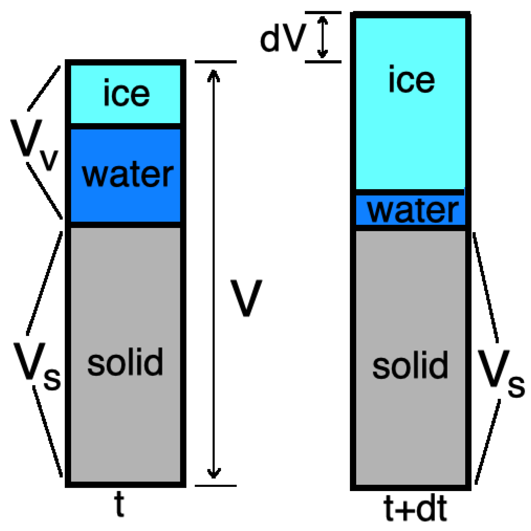
Let $T^t=T\left(t\right)$ and $T^{t+dt}=T(t+dt)$ be the temperature at times t and $t+dt$, where $dt$ is the time step. We define porosity at time t and $t+dt$ as follows (see Figure 2)

$${\varphi }_t=\frac{V_n}{V},{\varphi }_{t+dt}=\frac{V_n+dV}{V+dV},$$

where $dV$ is a change of volume.

The volumetric strain due to porosity change is given as follows (Zhang [30])

$$d{\epsilon }_v^{*}=\frac{dV}{V}.$$

Because

$${\varphi }_{t+dt}=\frac{V_n+dV}{V+dV}=\frac{\frac{V_n}{V}+\frac{dV}{V}}{1+\frac{dV}{V}}=\frac{{\varphi }_t+d{\epsilon }_v^{*}}{1+d{\epsilon }_v^{*}},$$

$${\varphi }_{t+dt}(1+d{\epsilon }_v^{*})={\varphi }_t+d{\epsilon }_v^{*},$$

we have

$$d{\epsilon }_v^{*}=\frac{{\varphi }_{t+dt}-{\varphi }_t}{1-{\varphi }_{t+dt}}=\frac{d\varphi }{1-\varphi },$$

where ${\varphi }_{t+dt}=\varphi$ is a current porosity and $d\varphi =({\varphi }_{t+dt}-{\varphi }_t)$ is porosity change.

For the linear elasticity model, we have

$$\mathrm{div}\left(d\sigma \right)=0,d\sigma =C:d\epsilon ,$$

where C is a stiffness tensor, $\sigma$ and $\epsilon$ are total stress and strain tensors, respectively.

The total strain is induced by loading and by a thermal process

$$d\epsilon =d{\epsilon }^e+d{\epsilon }^f,d{\epsilon }^f=\frac{1}{3}\mathcal{I}d{\epsilon }_v^f=\frac{1}{3}\mathcal{I}\frac{d\varphi }{1-\varphi },{\epsilon }^e=\frac{1}{2}(\nabla u+\nabla u^T),$$

where $d{\epsilon }^e$ is an elastic mechanical increment, $d{\epsilon }^f$ is a thermal porosity growth increment, $\mathcal{I}$ is the identity matrix and u is displacements.

For the two-dimensional isotropic media case, we have

$$\begin{array}{cc}\hfill d{\sigma }_{11}& =(\lambda +2\mu )d{\epsilon }_{11}^e+\lambda d{\epsilon }_{22}^e+\beta d\varphi ,{\epsilon }_{11}^e=\frac{\partial u_1}{\partial x_1},\hfill \\ \hfill d{\sigma }_{22}& =\lambda d{\epsilon }_{11}^e+(\lambda +2\mu )d{\epsilon }_{22}^e+\beta d\varphi ,{\epsilon }_{22}^e=\frac{\partial u_2}{\partial x_2},\hfill \\ \hfill d{\sigma }_{12}& =2\mu d{\epsilon }_{12}^e,{\epsilon }_{12}^e=\frac{1}{2}\left(\frac{\partial u_1}{\partial x_2}+\frac{\partial u_2}{\partial x_1}\right),\hfill \end{array}$$

and

$$\beta \left(T\right)=\frac{(3\lambda +2\mu )}{3(1-\varphi )},$$

where $u=(u_1,u_2)$, $\lambda$ and $\mu$ are Lame parameters, and $\beta$ is a thermal expansion due to porosity change.

In general, the following model for soils mechanics with phase change of porous water can be used

$$\mathrm{div}\left(d\sigma \right)=0,d\sigma =2\mu d{\epsilon }^e+\lambda \mathrm{tr}\left(d{\epsilon }^e\right)\mathcal{I}+\beta d\varphi \mathcal{I},$$

where ${\epsilon }^e=(\nabla u+\nabla u^T)/2$.

3.3. Thermo-Mechanical Model

Finally, we obtain the following thermo-mechanical model in the computational domain $\Omega$

$$\begin{array}{cc}\hfill & \left(c\rho +D{w}^{\prime }\right)\frac{\partial T}{\partial t}-\nabla ·(k\nabla T)=0,x\in \Omega ,t>0,\hfill \end{array}$$

(11a)

$$\begin{array}{cc}\hfill & \nabla (\mu \nabla du)+\nabla [(\lambda +\mu )\nabla ·du]+\nabla \left(\beta d\varphi \right)=0,x\in \Omega ,t>0.\hfill \end{array}$$

(11b)

The system of Equations (11a) and (11b) is an uncoupled system of equations because the presented model neglects the influence of the displacement field on the temperature distribution. In general, the mathematical model can be constructed in a coupled way with an additional part that takes into account the influence of the deformation on the temperature field. In this work, we investigate and implement a simplified model, where the temperature does not depend on displacements and can be calculated first. After using the calculated temperature field, we can find the value of porosity change $d\varphi$ to calculate a correspondent displacement field of soils.

We consider the thermo-mechanical model with the following initial conditions

$$T=T_0,u=u_0,x\in \Omega ,t=0$$

(12)

and boundary conditions

$$\begin{array}{cc}\hfill & -k\nabla T·n=0,x\in {\Gamma }_1,-k\nabla T·n=\gamma (T-T_1),x\in {\Gamma }_2,\hfill \end{array}$$

(13a)

$$\begin{array}{cc}\hfill & \sigma ·n=0,x\in {\Gamma }_3,u=0,x\in {\Gamma }_4.\hfill \end{array}$$

(13b)

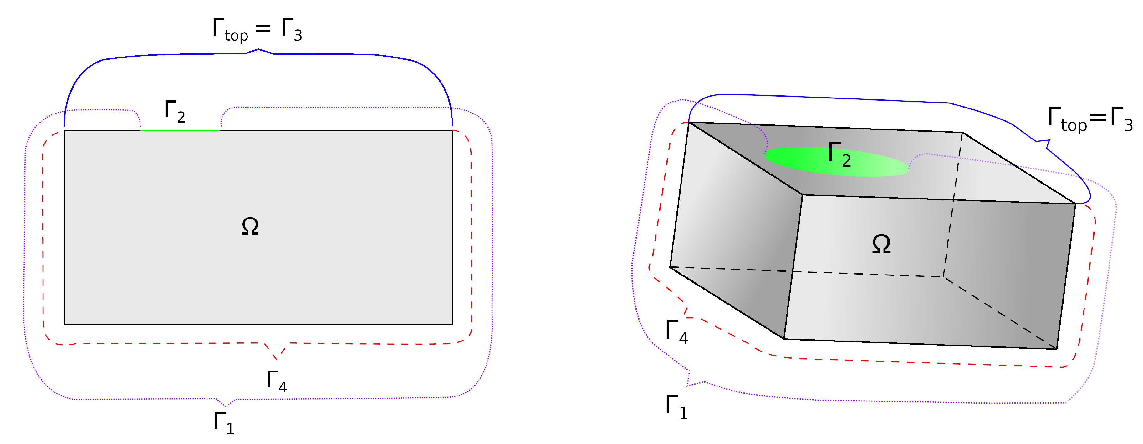
where n is the outward unit normal vector to $\partial \Omega$ and ${\Gamma }_1\cup {\Gamma }_2={\Gamma }_3\cup {\Gamma }_4=\partial \Omega$. Note that in (12), (13a) and (13b) the general formulation of the initial and boundary conditions is presented. In Figure 3, we present one possible variant of the domain $\Omega$ and the boundaries for which we can set such conditions. In this variant, we set ${\Gamma }_2\subset {\Gamma }_{top}$ (green color), and ${\Gamma }_1=\partial \Omega \backslash {\Gamma }_2$ (purple color), and ${\Gamma }_3={\Gamma }_{top}$ (blue color), and ${\Gamma }_4=\partial \Omega \backslash {\Gamma }_3$ (red color).

The presented basic mathematical model (11a) and (11b), is the simplification of the model presented in (Zhang [30]). We use the presented model to illustrate the influence of the water/ice phase-change in porous media on deformations of the soils. Next, we will present a finite element approximation of the thermoelastic model with porous water/ice phase-change. In the numerical implementation, we don’t use a proprietary “black box” software and present an openly available implementation based on the FEniCS library using a C++ programming language for fast simulations of multidimensional problems.

4. Finite Element Approximation

For the numerical solution of the mathematical model, we use a finite element method with implicit time approximation (Brenner and Scott [31], Kolesov et al. [37], Vasilyeva et al. [38]). We start with variational formulation of the problem (11a), (11b), (13a) and (13b) with initial conditions (12). Then, the formulation of the discrete problem is presented in matrix form.

4.1. Variational Formulation

Let

$$V\in \{v\in {\left[H_1(\Omega )\right]}^d:v\left(x\right)=0,x\in {\Gamma }_4\},$$

and $Q=H{}_1(\Omega )$ be the functional spaces for displacements and temperature, $T\in Q$ and $u\in V$, where $H_1(\Omega )$ is a Hilbert space, $H_1(\Omega )=\{v\in L_2(\Omega )|\frac{\partial v}{\partial x_i}\in L_2(\Omega ),i=1,...,d\}$ ($d=2,3$ is the dimension of the problem).

Multiplying (11a) and (11b) by test functions $r\in Q$ and $v\in V$, respectively, and integrating by parts with boundary conditions given by (13a) and (13b), we obtain the following variational formulation of the thermo - mechanical problem (Brenner and Scott [31]): find $T\in Q$ and $u\in V$ such that

$$\begin{array}{cc}\hfill & {\int }_{\Omega }(c\rho +D{w}^{\prime })\frac{\partial T}{\partial t}rdx+{\int }_{\Omega }k\nabla T·\nabla rdx+{\int }_{{\Gamma }_2}\gamma (T-T_1)rdx=0,\forall r\in Q,\hfill \end{array}$$

(14a)

$$\begin{array}{cc}\hfill & {\int }_{\Omega }d\sigma \left(u\right):\epsilon \left(v\right)dx+{\int }_{\Omega }\nabla \left(\beta d\varphi \right)vdx=0,\forall v\in V,\hfill \end{array}$$

(14b)

where operator: is the inner product between tensors. For approximation by time, the Backward Euler scheme is used

$$\frac{\partial T}{\partial t}\approx \frac{T^{m+1}-T^m}{\tau },$$

where $\tau$ is the size of the time step, and m is a time step number, $m=0,1,...,N_t$.

Therefore, the variational formulation is the following: find $T^{m+1}\in Q$ and $u^{m+1}\in V$ such that

$$\begin{array}{cc}\hfill {\int }_{\Omega }\left[{\left(c\rho \right)}^{m+1}+{\left(D{w}^{\prime }\right)}^{m+1}\right]\frac{T^{m+1}-T^m}{\tau }rdx& +{\int }_{\Omega }{k}^{m+1}\nabla T^{m+1}·\nabla rdx\hfill \\ & +{\int }_{{\Gamma }_2}\gamma (T^{m+1}-T_1)rdx=0,\forall r\in Q,\hfill \\ \hfill {\int }_{\Omega }[\sigma \left(u^{m+1}\right)-\sigma \left(u^m\right)]:\epsilon \left(v\right)dx& +{\int }_{\Omega }\nabla \left[\beta \left(T^{m+1}\right)({\varphi }^{m+1}-{\varphi }^m)\right]vdx=0,\forall v\in V,\hfill \end{array}$$

where ${\left(c\rho \right)}^{m+1}=c\rho \left(T^{m+1}\right)$, ${\left(D{w}^{\prime }\right)}^{m+1}=D\left(T^{m+1}\right)w^{\prime }\left(T^{m+1}\right)$, $k^{m+1}=k\left(T^{m+1}\right)$ and ${\beta }^{m+1}=\beta \left(T^{m+1}\right)$.

Because, in our model, the heat equation does not depend on deformations, we can split the heat equation from the mechanical model.

To solve the nonlinear problem for temperature, the Picard iterative process is used (Logg et al. [35]). At each time layer, we solve the following linear system of equations:

$$\begin{array}{cc}\hfill {\int }_{\Omega }\left[{\left(c\rho \right)}^{m+1,l}+{\left(D{w}^{\prime }\right)}^{m+1,l}\right]\frac{T^{m+1,l+1}-T^m}{\tau }rdx& +{\int }_{\Omega }{k}^{m+1,l}\nabla T^{m+1,l+1}·\nabla rdx\hfill \\ & +{\int }_{{\Gamma }_2}\gamma (T^{m+1,l+1}-T_1)rdx=0,\hfill \end{array}$$

where l is the number of nonlinear iteration ($l=0,N_{nl}$) and initial guess $T^{m+1,0}=T^m$. In order to stop iterations, we calculate the relative difference in $L_2$ norm and use the following criteria

$$\frac{\parallel T^{m+1,l}-T^{m+1,l}{\parallel }_{L_2}}{\parallel T^{m+1,l}{\parallel }_{L_2}}\times 100\%<ϵ,$$

(15)

where relative tolerance $ϵ$ is given in % and ${\parallel v\parallel }_{L_2}=\sqrt{{\int }_{\Omega }{v}^{2}dx}$.

We get the following algorithm:

• Find $T^{m+1,l+1}\in Q$ such that:

  $$s^{m+1,l}(T^{m+1,l+1},r)+a_T^{m+1,l}(T^{m+1,l+1},r)=s^{m+1,l}(T^m,r)+l\left(r\right),\forall r\in Q,$$

  (16)

  where

  $$s^{m+1,l}(T,r)=\frac{1}{\tau }{\int }_{\Omega }\left[{\left(c\rho \right)}^{m+1,l}+{\left(D{w}^{\prime }\right)}^{m+1,l}\right]Trdx,$$

  $$a_T^{m+1,l}(T,r)={\int }_{\Omega }{k}^{m+1,l}\nabla T·\nabla rdx+{\int }_{{\Gamma }_2}\gamma Trdx,l\left(r\right)={\int }_{{\Gamma }_2}\gamma T_{1}rdx.$$

  with convergence criteria (15) and $T^{m+1}=T^{m+1,l+1}$.
• Find $u^{m+1}\in V$ such that:

  $$a_u(u^{m+1},v)=a_u(u^m,v)+b(T^{m+1},v)-b(T^m,v),\forall v\in V,$$

  (17)

  where

  $$a_u(u,v)={\int }_{\Omega }\sigma \left(u\right):\epsilon \left(v\right)dx,b(T,v)={\int }_{\Omega }\left[\beta \left(T\right)\varphi \left(T\right)\mathcal{I}\right]:\epsilon \left(v\right)dx,$$

  and porosity is the function of temperature

  $$\varphi \left(T\right)=\frac{w\frac{{\rho }_s}{{\rho }_w}+(\overline{w}-w\left(T\right))\frac{{\rho }_s}{{\rho }_i}}{1+w\left(T\right)\frac{{\rho }_s}{{\rho }_w}+(\overline{w}-w\left(T\right))\frac{{\rho }_s}{{\rho }_i}}.$$

  where

  $$w\left(T\right)=\left\{\begin{array}{cc}\overline{w},\hfill & T\ge T_f,\hfill \\ w^{*}+(\overline{w}-w^{*})exp\left(a[T-T_f]\right),\hfill & T<T_f.\hfill \end{array}\right.$$

Here $\sigma \left(u\right)=2\mu \epsilon +\lambda \mathrm{tr}\left(\epsilon \right)\mathcal{I}$ and $\epsilon =(\nabla u+\nabla u^T)/2$.

4.2. Finite Element Discretization

Let ${\mathcal{T}}^h$ be a grid partition of the computational domain $\Omega$ into finite elements $K_i$

$${\mathcal{T}}^h={\cup }_i{K}_i,i=1,\dots N_c,$$

where $N_c$ is a number of grid cells. Relative to ${\mathcal{T}}^h$, we define finite-dimensional spaces $V_h\subset V$ and $Q_h\subset Q$. We suppose that $Q_h$ and $V_h$ are composed of piecewise linear basis functions on grid cells (Brenner and Scott [31], Logg et al. [35])

$$Q_h=\mathrm{span}\{{\phi }_j,j=1,...,N_T\},V_h=\mathrm{span}\{{\psi }_j,j=1,...,N_u\},$$

where ${\psi }_j$ and ${\phi }_j$ are linear basis functions defined on ${\mathcal{T}}^h$, $N_u=\dim \left(V_h\right)$ and $N_T=\dim \left(Q_h\right)$. Note that $N_T=N$ and $N_u=d·N$ for linear basis functions, where N is the number of vertices, and d is the dimension of the problem ($d=2,3$). Functions $u_h$ and $T_h$ can be represented using decomposition on the basis of $V_h$ and $Q_h$

$$T_h\left(x\right)=\sum _{j=1}^{N_T}{T}_j{\phi }_j\left(x\right),u_h\left(x\right)=\sum _{j=1}^{N_u}{u}_j{\psi }_j\left(x\right).$$

Thus, we obtain the following discrete systems in matrix form:

• Solve the heat equation for $T^{m+1}={(T_1^{m+1},...,T_{N_T}^{m+1})}^T$

  $$(S^{m+1,l}+A_T^{m+1,l})T^{m+1,l+1}=S^{m+1,l}{T}^m+F,$$

  where $S^{m+1,l}=\left[s_{ij}^{m+1,l}\right]$, $A_T^{m+1,l}=\left[a_{T,ij}^{m+1,l}\right]$, $F_T=\left\{f_j\right\}$ and

  $$s_{ij}^{m+1,l}=s^{m+1,l}({\phi }_i,{\phi }_j),a_{T,ij}^{m+1,l}=a_T^{m+1,l}({\phi }_i,{\phi }_j),f_j=l\left({\phi }_j\right).$$
• Solve the displacement equation for $U^{m+1}={(u_1^{m+1},...,u_{N_u}^{m+1})}^T$

  $$A_u{U}^{m+1}=A_u{U}^m+B^{m+1}-B^m,$$

  where $A_u=\left[a_{u,ij}\right]$, $B^m=\left\{b_j^m\right\}$,

  $$a_{u,ij}=a_u({\psi }_i,{\psi }_j),b_j^m=b(T^m,{\psi }_j).$$

In the presented algorithm, we first solve a temperature equation using the Picard iterative method. Then, we find displacements for the given temperature change.

For the implementation of the presented basic mathematical model with finite element approximation, we use the FEniCS finite element software (Logg et al. [35]) (version 2019.1.0+). The FEniCS library is a tool for automated scientific computing, with a particular focus on the solution of differential equations by the finite element method. The code for the presented thermoelastic model is written using C++ Programming Language to perform fast calculations of multidimensional problems. We use the GMSH program to construct computational geometries, and unstructured grids (Geuzaine and Remacle [41]). Paraview program is used for visualization of the results (Ahrens et al. [42]). The code and geometry files are openly available on Bitbucket at https://bitbucket.org/vmasha/thermoelastic/.

5. Numerical Results

In this section, we present the results of numerical simulations for two- and three-dimensional model problems. In particular, we numerically examine the presented approximation for different time step sizes and their influences on the number of nonlinear iterations. We present errors for temperature and displacements between the given solution and reference solution using a smaller number of time steps. Finally, we discuss the computational time of the presented implementation.

Phase-change parameters

$$L=333000\mathrm{J}·{\mathrm{kg}}^{-1},T_f=0.0{ }^{°}\mathrm{C}.$$

For the unfrozen water content model (1), we set

$$w\left(T\right)=\left\{\begin{array}{cc}\overline{w},\hfill & T\ge T_f,\hfill \\ w^{*}+(\overline{w}-w^{*})exp\left(a\right[T-T_f\left]\right),\hfill & T<T_f\hfill \end{array}\right.$$

with $w^{*}=0$, $\overline{w}=0.0285$, and $a={\left(0.3\right)}^{-1}$${ }^{°}{\mathrm{C}}^{-1}$. Illustration of water fraction volume ${\Theta }_w$, ice fraction volume ${\Theta }_i$ and porosity $\varphi$ is presented in Figure 4.

We set the following parameters (Zhang [30])

• solid:

  $${\rho }_s=2620\mathrm{kg}·{\mathrm{m}}^{-3},c_s=900\mathrm{J}·{\mathrm{kg}}^{-1}·{ }^{°}{\mathrm{C}}^{-1},k_s=0.95\mathrm{W}·{\mathrm{m}}^{-1}·{ }^{°}{\mathrm{C}}^{-1},$$
• water:

  $${\rho }_w=1000\mathrm{kg}·{\mathrm{m}}^{-3},c_w=4180\mathrm{J}·{\mathrm{kg}}^{-1}·{ }^{°}{\mathrm{C}}^{-1},k_w=0.56\mathrm{W}·{\mathrm{m}}^{-1}·{ }^{°}{\mathrm{C}}^{-1},$$
• ice:

  $${\rho }_i=917\mathrm{kg}·{\mathrm{m}}^{-3},c_i=2000\mathrm{J}·{\mathrm{kg}}^{-1}·{ }^{°}{\mathrm{C}}^{-1},k_i=2.24\mathrm{W}·{\mathrm{m}}^{-1}·{ }^{°}{\mathrm{C}}^{-1}.$$

We set the following elastic parameters

$$\lambda =\frac{\nu E}{(1+\nu )(1-2\nu )},\mu =\frac{E}{2(1+\nu )},$$

with $E=50\times {10}^6\mathrm{Pa}$ and $\nu =0.3$.

5.1. Two-Dimensional Problem

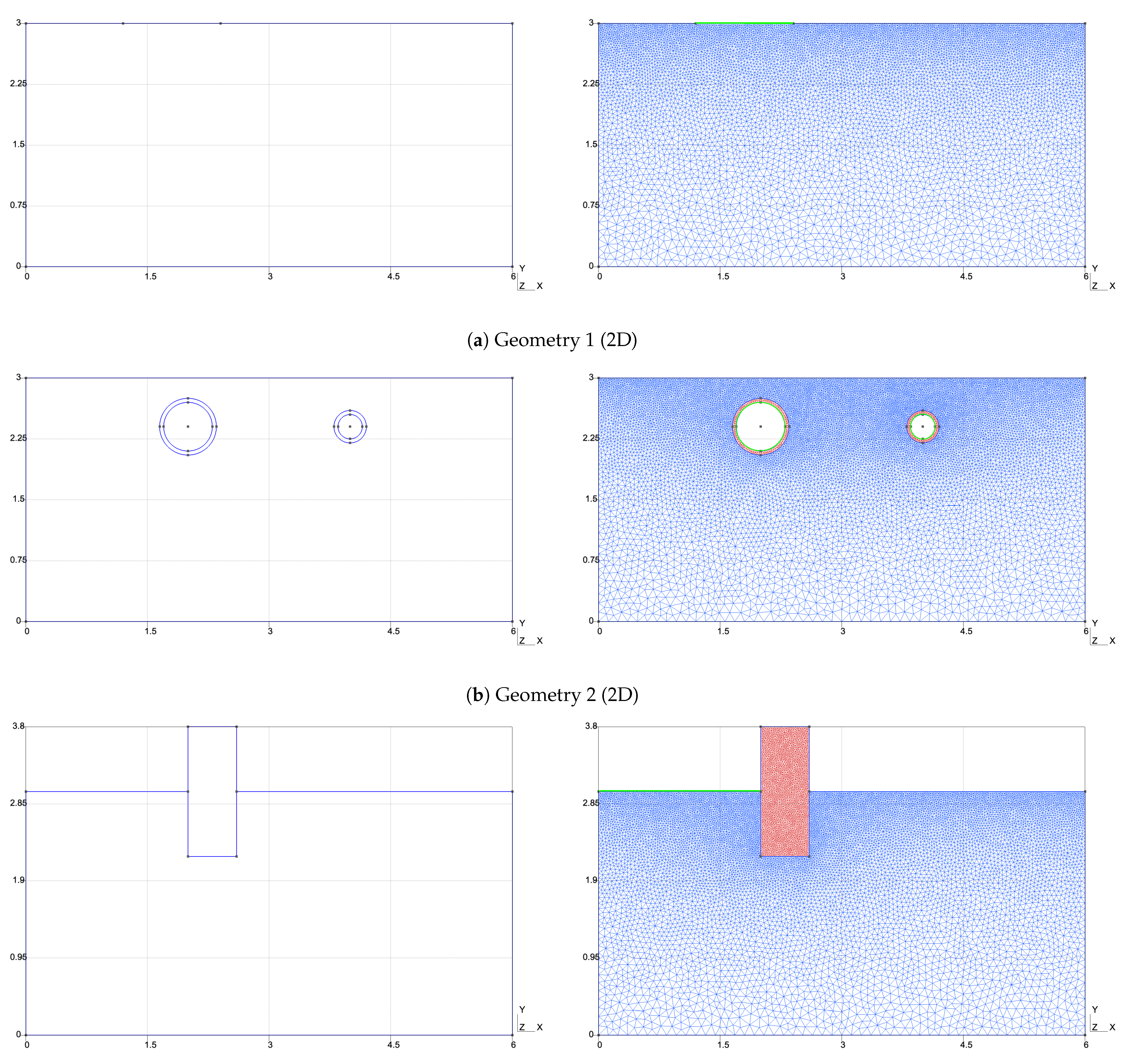
In this section, we present numerical results for the two-dimensional domain $\Omega$.

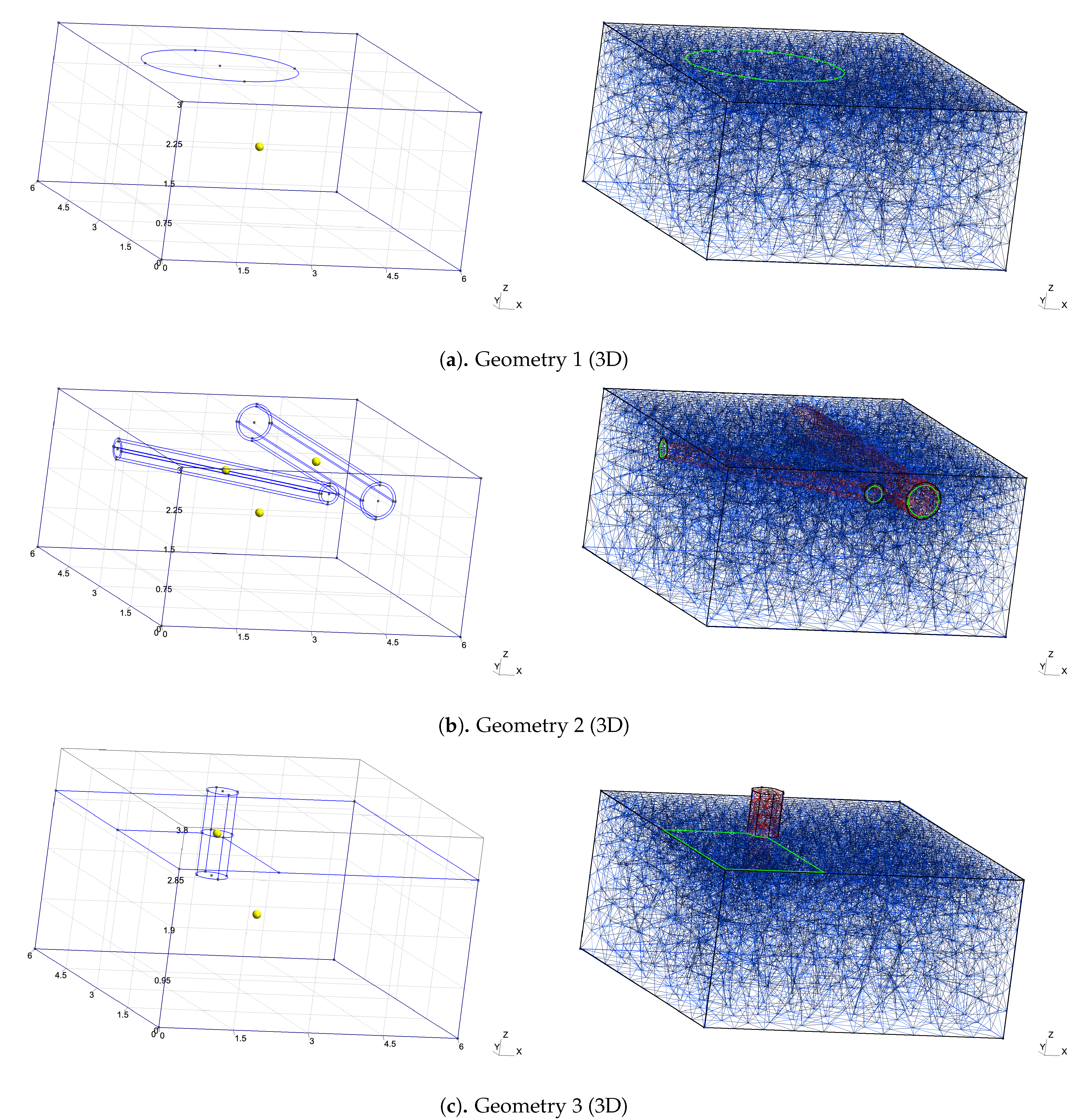
Three geometries of the computational domain are considered:

• Geometry 1 (see Figure 5a).

Rectangular domain $\Omega =[0,L_x]\times [0,L_y]$ with $L_x=6$ m and $L_y=3$ m. On the boundary ${\Gamma }_H$ (green line), we set temperature $T_1=T_H$ and $T_1=T_C$ on the top boundary ${\Gamma }_C={\Gamma }_{top}/{\Gamma }_H$.

• Geometry 2 (see Figure 5b).

Rectangular domain with two perforations (pipes) $\Omega ={\Omega }_m/{\Omega }_p$, where ${\Omega }_m=[0,L_x]\times [0,L_y]$ with $L_x=6$ m and $L_y=3$ m and ${\Omega }_p$ is the two circle domains. Two subdomains have different properties ($\Omega ={\Omega }_1\cup {\Omega }_2$), where ${\Omega }_1$ is the subdomain of soil (blue color in Figure 5b) and ${\Omega }_2$ is the subdomain of pipe walls (red color). On the boundary of pipes ${\Gamma }_H=\partial \Omega \cap \partial {\Omega }_2$ (green line), we set temperature $T_1=T_H$ and $T_1=T_C$ on the top boundary ${\Gamma }_C={\Gamma }_{top}$.

• Geometry 3 (see Figure 5c).

Computational domain with two subdomains $\Omega ={\Omega }_1\cup {\Omega }_2$, where ${\Omega }_1$ is the subdomain of soil (blue color in Figure 5c), and ${\Omega }_2$ is the subdomain of the pillar (red color). On the green boundary ${\Gamma }_H$, we set temperature $T_1=T_H$ and $T_1=T_C$ on other top boundary ${\Gamma }_C={\Gamma }_{top}/{\Gamma }_H$.

In second subdomain ${\Omega }_2$, we simulate stiff material $E_2={10}^{11}\mathrm{Pa}$, ${\nu }_2=0.3$ with low heat conductivity $k_2=1\mathrm{W}·{\mathrm{m}}^{-1}·{ }^{°}{\mathrm{C}}^{-1}$ and ${\rho }_2=2620\mathrm{kg}·{\mathrm{m}}^{-3}$, $c_2=900\mathrm{J}·{\mathrm{kg}}^{-1}·{ }^{°}{\mathrm{C}}^{-1}$.

Two-dimensional domains with unstructured grids are represented in Figure 5. The first geometry (Figure 5a) shows a thawing process caused by positive temperature on the boundary. This example illustrates the impact of a building/construction on the soil when poor floor insulation causes thawing during the winter period. The second geometry in Figure 5b illustrates the impact of underground pipes filled with warm water. This example shows how warm temperature can change the temperature field around and lead to thawing if poorly insulated. The third geometry (Figure 5c) illustrates deformation and heat transfer under the building/construction, where subdomain ${\Omega }_2$ is the construction pillar. The example represents temperature changes under the construction and affects the pillar.

Unstructured meshes are constructed with local refinement near boundaries ${\Gamma }_C$ and ${\Gamma }_H$. Computational mesh sizes and the number of degrees of freedom are the following:

• Geometry 1: mesh contains 8580 vertices and 16,756 cells, $DO{F}_T=8580$ and
  $DO{F}_u$ = 17,160.
• Geometry 2: mesh contains 13,012 vertices and 25,504 cells, $DO{F}_T$ = 13,012 and
  $DO{F}_u$ = 26,024.
• Geometry 3: mesh contains 12,417 vertices and 24,361 cells, $DO{F}_T$ = 12,417 and
  $DO{F}_u$ = 24,834.

We simulate for $t_{max}={10}^6\mathrm{s}$ with two initial conditions for temperature:

• Test 1. Frozen initial condition with $T_0=-2°\mathrm{C}$.
• Test 2. Unfrozen initial condition with $T_0=2°\mathrm{C}$.

As boundary conditions, we set Robin boundary conditions on ${\Gamma }_C$ and ${\Gamma }_H$

$$-k\nabla T·n={\gamma }_C(T-T_C),x\in {\Gamma }_C,-k\nabla T·n={\gamma }_H(T-T_H),x\in {\Gamma }_H,$$

with $T_C=-15{}^{°}\mathrm{C}$, ${\gamma }_C=14\mathrm{W}·{\mathrm{m}}^{-2}·{}^{°}{\mathrm{C}}^{-1}$, $T_H=10{}^{°}\mathrm{C}$ and ${\gamma }_H=20\mathrm{W}·{\mathrm{m}}^{-2}·{}^{°}{\mathrm{C}}^{-1}$. On other boundaries $\partial \Omega /({\Gamma }_C\cup {\Gamma }_H)$, we set zero Neumann boundary conditions. For displacements, we set ${\sigma }_1=0\mathrm{Pa}$$u_2=0\mathrm{m}$ on the bottom boundary, and $u_1=0\mathrm{m}$, ${\sigma }_2=0\mathrm{Pa}$ on the left and right boundary. As initial condition, we set $u_0=0\mathrm{m}$.

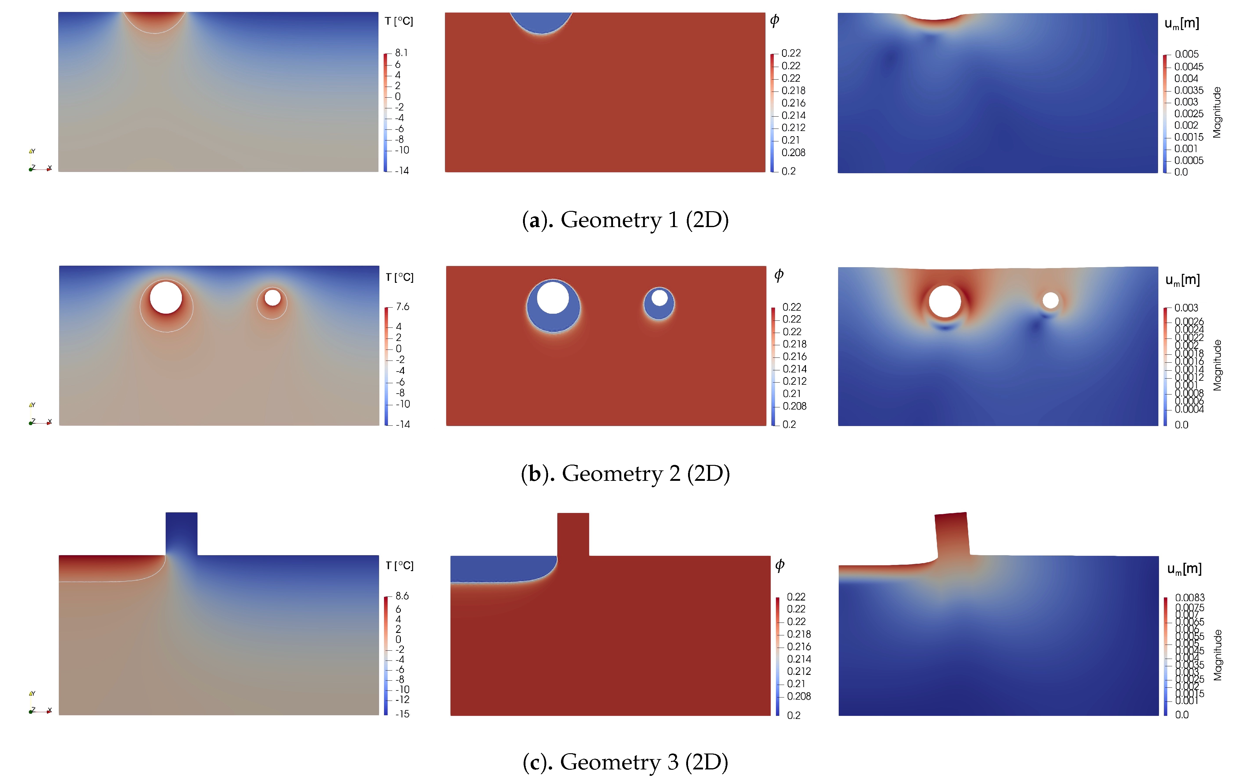
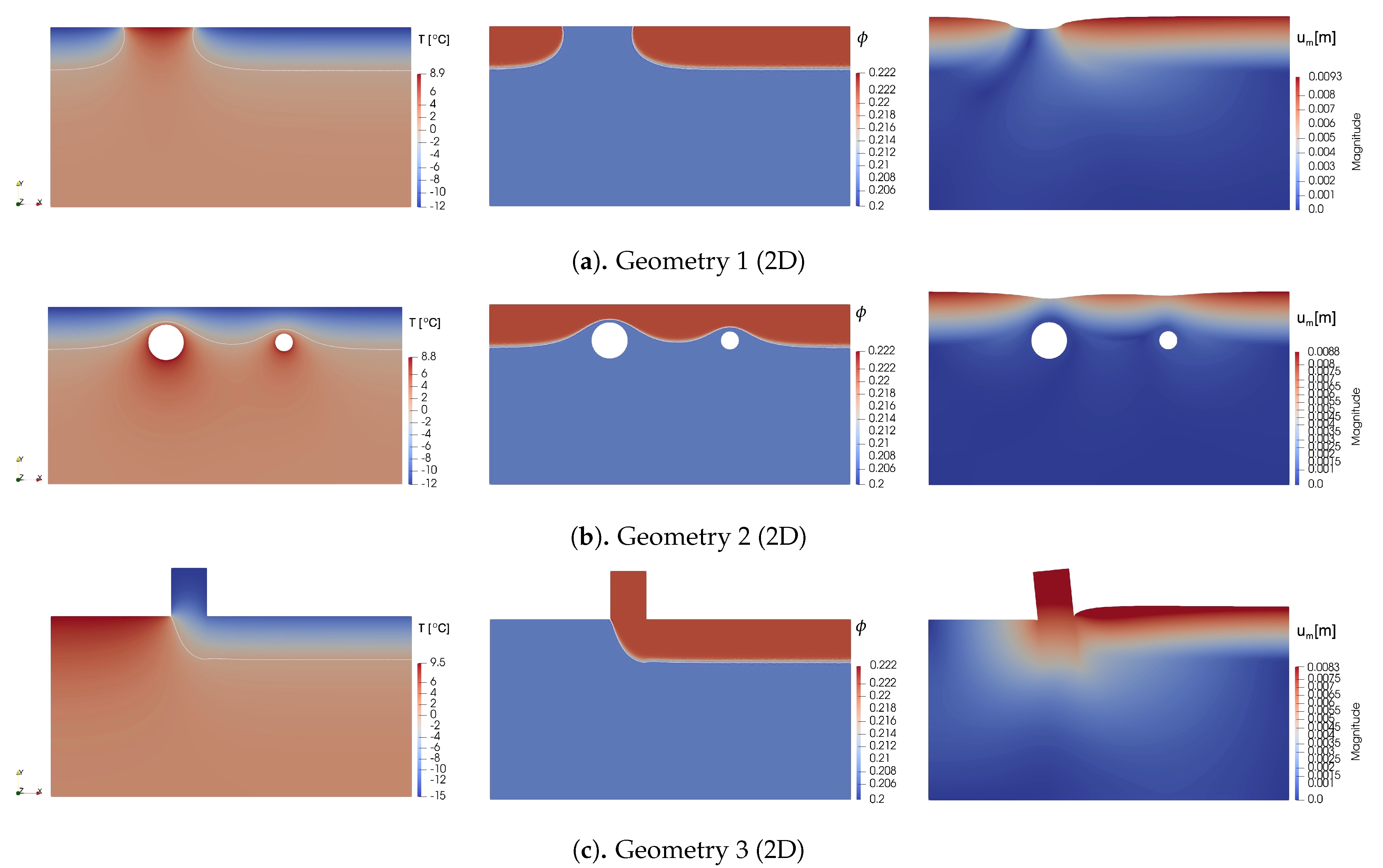
Numerical results for Test 1 are presented in Figure 6 and for Test 2 in Figure 7. Results have been performed with 300 time steps using Picard iterations with $ϵ=1\%$. On the left figure, we presented a temperature field distribution at the final time. The corresponding porosity field is shown in the middle figure. On the right figure, we depict a magnitude of displacements field on the moved mesh, where displacements are exaggerated by a factor of 25. The temperature field and porosity are depicted with the phase-change interface (white color line).

In Figure 6, we depicted results for Test 1 with frozen initial condition for temperature, $T_0=-2{}^{°}\mathrm{C}$. On the left figures, we observe the thawing process near the boundary ${\Gamma }_H$, where we set Robin boundary conditions with temperature, $T_1=10{}^{°}\mathrm{C}$. On the right figures, we see nearly vertical displacements caused by soil thawing. The results in Figure 6 illustrates the impact of a building/construction or pipes on the soil when poor floor insulation causes thawing during the winter period. We observe how warm temperature can change the temperature field around and lead to thawing if poorly insulated. The thawing has changed the porosity field as pore water has a larger density, and it occupies a smaller volume and leads to soil deformations.

The results of the numerical simulations for Test 2 are presented in Figure 7. In this example, we consider a case with unfrozen initial condition for temperature, $T_0=2{}^{°}\mathrm{C}$. By setting freezing boundary conditions on the top boundary ${\Gamma }_H$, we simulate the influence of the different constructions on the temperature and displacements fields. From this example, we observe how different boundary conditions on ${\Gamma }_C$ and ${\Gamma }_H$ affect the phase-change interface. From the middle figures of the porosity field related to the temperature at the final time, we observe porosity change due to freezing of the pore water. The right figures show displacements that occur for the given porosity change.

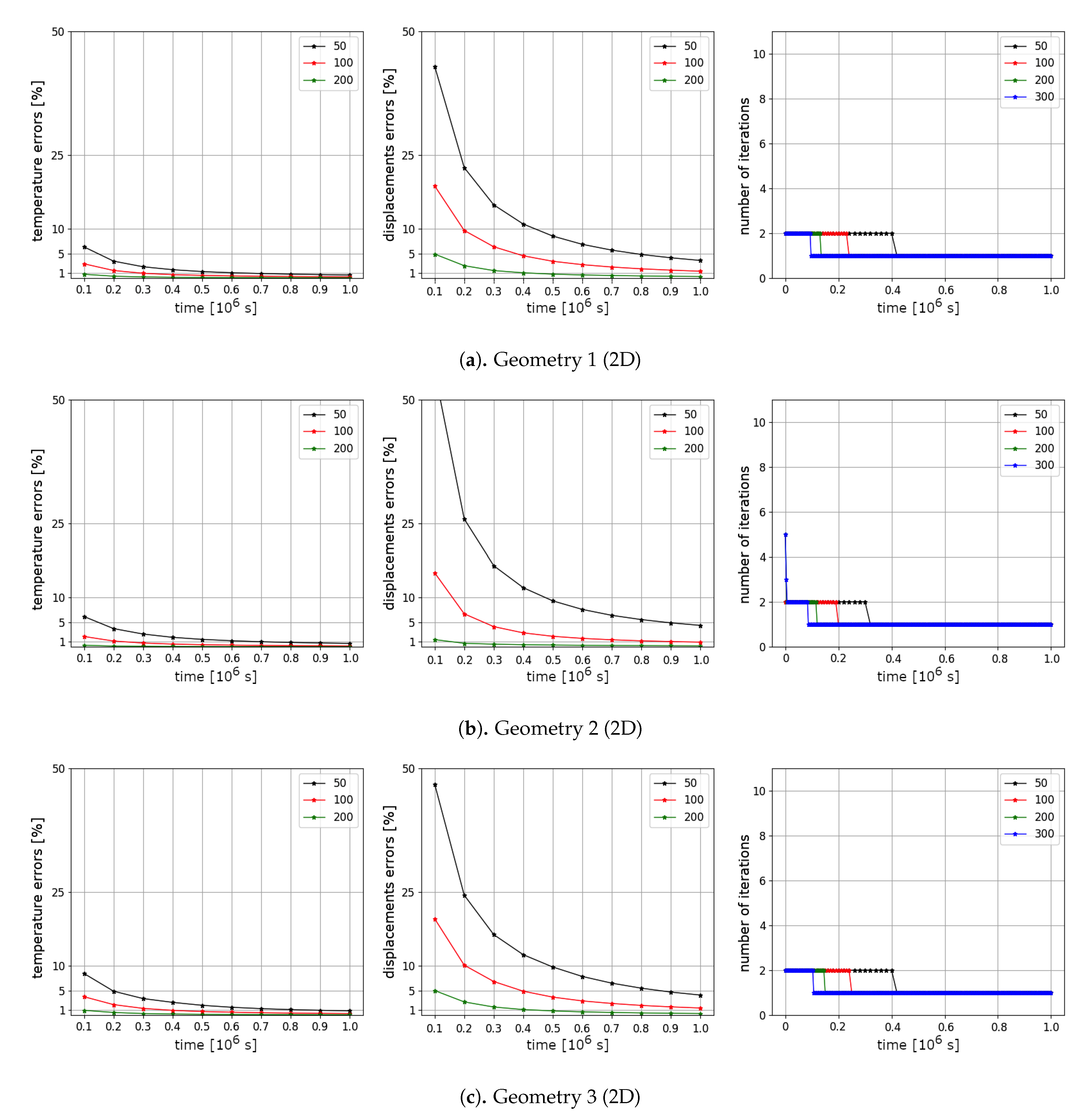
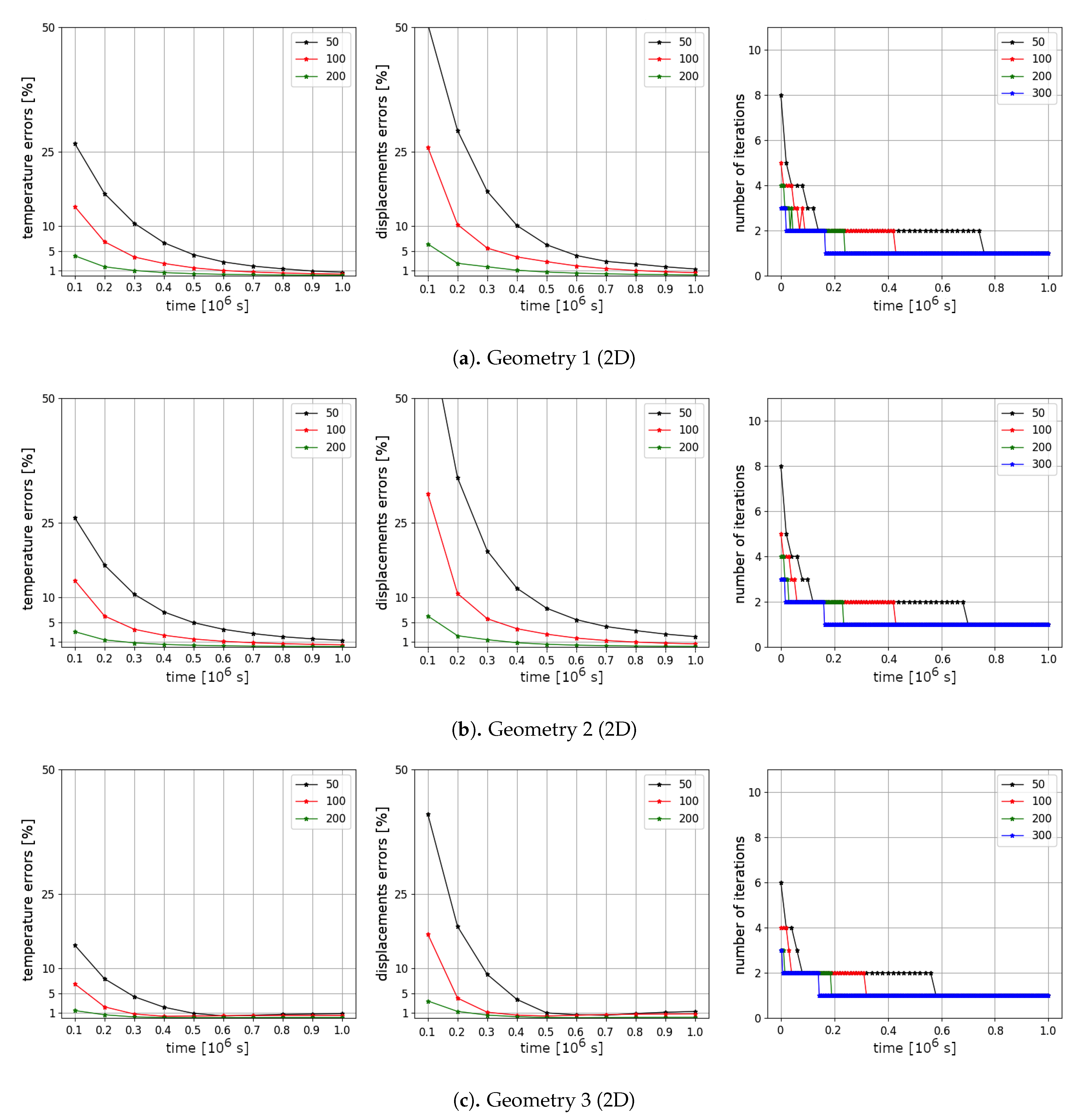
Next, we numerically investigate the solution of the problem using Picard iterations with a different number of time steps $N_t=50,100,200$. To compare the difference between solutions with different time steps, we calculate relative $L_2$ errors in %

$$e_T=\frac{\parallel T-T_{ref}{\parallel }_{L_2}}{\parallel T_{ref}{\parallel }_{L_2}}\times 100\%,e_u=\frac{\parallel u-u_{ref}{\parallel }_{L_2}}{\parallel u_{ref}{\parallel }_{L_2}}\times {100\%,\parallel v\parallel }_{L_2}=\sqrt{{\int }_{\Omega }{v}^{2}dx},$$

where $T_{ref}$ and $u_{ref}$ are reference solutions. Because we cannot calculate the analytical solution for the considered geometries in two and three-dimensional formulations, as the reference solutions in order to investigate numerical convergence of the presented algorithm with a different number of time steps and calculate errors, we use numerical results for $N_t=300$ with Picard iterations.

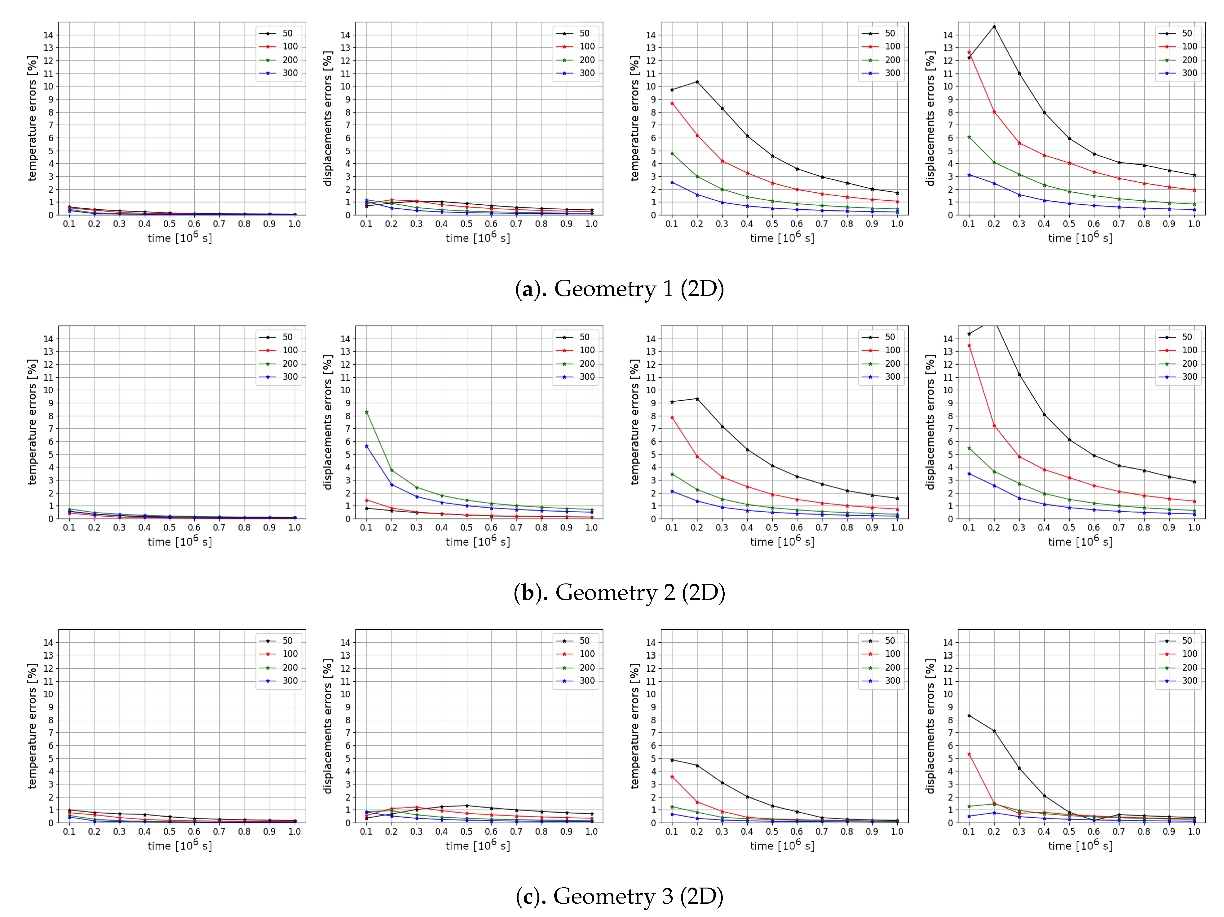
In Figure 8 and Figure 9, we present relative errors in % for 10 time layers using Picard iterations for Test 1 and Test 2, respectively. In the first and second columns, relative errors for temperature and displacements are depicted. In the third column, the number of Picard iterations are presented for each time step. We observe the influence of the time step size on the solutions and have the following conclusions from the presented results:

• From the first and second columns in Figure 8 and Figure 9, we observe larger errors for Test 2 than for Test 1 for all computational domains at initial time layers. For example, in Geometry 1 using $N_t=50$ time iterations, we have $(6.3\%,3.4\%,2.2\%)$ of temperature errors in Test 1 and $(26.6\%,16.5\%,10.5\%)$ of temperature errors in Test 2 at times $t=(0.1,0.2,0.3)\left[{10}^6\mathrm{s}\right]$, respectively. For displacements errors, we have $(42.9\%,22.3\%,14.8\%)$ in Test 1 and $(50.6\%,29.2\%,16.9\%)$ in Test 2 at times $t=(0.1,0.2,0.3)\left[{10}^6\mathrm{s}\right]$, respectively. When we use more iterations by time for Geometry 1 ($N_t=200$), we have $(0.7\%,0.3\%,0.2\%)$ of temperature errors in Test 1 and $(4.0\%,1.7\%,1.0\%)$ of temperature errors in Test 2 at times $t=(0.1,0.2,0.3)\left[{10}^6\mathrm{s}\right]$, respectively. For displacements errors, we have $(4.8\%,2.5\%,1.5\%)$ in Test 1 and $(6.3\%,2.4\%,1.7\%)$ in Test 2 at times $t=(0.1,0.2,0.3)\left[{10}^6\mathrm{s}\right]$, respectively. At the final time, we obtain good results with less than one percent of errors for temperature and displacements using $N_t=100$ and 200 for all Geometries.
• The influence of the time step size is larger for displacements than for temperature for both tests (see Figure 8 and Figure 9). For example, in Test 1 (Geometry 1) at the final time, we have $(0.6\%,0.2\%,0.06\%)$ of temperature errors and $(3.5\%,1.3\%,0.3\%)$ of displacements errors for $N_t=(50,100,200)$, respectively. In Test 2 for Geometry 1 at the final time, we have $(0.7\%,0.3\%,0.09\%)$ of temperature errors and $(1.3\%,0.6\%,0.1\%)$ of displacements errors for $N_t=(50,100,200)$, respectively. Furthermore, the displacements errors are larger than the temperature errors at initial time layers. For example, in Test 1 using $N_t=100$ time iterations (Geometry 1) we have $(2.8\%,1.5\%,0.9\%)$ of temperature errors and $(18.6\%,9.6\%,6.3\%)$ of displacements errors at times $t=(0.1,0.2,0.3)\left[{10}^6\mathrm{s}\right]$, respectively. We observe similar error behavior for the second and the third geometries.
• Figure 8 and Figure 9 show that errors decrease by time for Test 1 and 2 in all computational domains. For example, the temperature error decreases from $2.8\%$ at time $t_m=0.1\left[{10}^6\mathrm{s}\right]$ to $0.2\%$ at the final time and displacements error decreases from $18.6\%$ at time $t_m=0.1\left[{10}^6\mathrm{s}\right]$ to $1.3\%$ at the final time for Test 1 using $N_t=100$ time iterations (Geometry 1). In Test 2 using $N_t=100$ time iterations (Geometry 1), the temperature error decreases from $13.9\%$ at time $t_m=0.1\left[{10}^6\mathrm{s}\right]$ to $0.3\%$ at the final time and displacements error decreases from $25.8\%$ at time $t_m=0.1\left[{10}^6\mathrm{s}\right]$ to $0.6\%$ at the final time.
• From the third column in Figure 8 and Figure 9, we observe that nonlinear iterations have good convergence for Test 1 and 2 for all geometries, where more iterations are needed at the first time steps. For Geometry 1, we observe that 42 % of all time iterations perform more than one nonlinear iteration (21 time iterations from total 50, till $t=0.42\left[{10}^6\mathrm{s}\right]$) for $N_t=50$, 24 % for $N_t=100$ (24 from 100, till $t=0.24\left[{10}^6\mathrm{s}\right]$), 13.5 % for $N_t=200$ (27 from 200, till $t=0.135\left[{10}^6\mathrm{s}\right]$), and 9.6 % for $N_t=300$ (29 from 300, till $t=0.096\left[{10}^6\mathrm{s}\right]$) in Test 1. In Test 2 (Geometry 1), we observe that 76 % of all time iterations perform more than one nonlinear iteration (38 time iterations from total 50, till $t=0.76\left[{10}^6\mathrm{s}\right]$) for $N_t=50$, 43 % for $N_t=100$ (43 from 100, till $t=0.43\left[{10}^6\mathrm{s}\right]$), 24 % for $N_t=200$ (48 from 200, till $t=0.24\left[{10}^6\mathrm{s}\right]$), and 16.6 % for $N_t=300$ (50 from 300, till $t=0.16\left[{10}^6\mathrm{s}\right]$). We obtain similar behavior for Geometry 2 and 3 and see that the Picard iterative method needs more iterations to converge for a small number of time steps $N_t$.

In Figure 10, we present the difference between solution using linearization from the previous time layer (one Picard iteration) and solution using Picard iterations using the same numbers for time steps $N_t=50,100,200$, and 300. We obtain the following conclusions:

• For Test 1, we have a small difference between solution using linearization from the previous time layer and solution using Picard iterations. For example, in Test 1 (Geometry 1), we have near or less than one percent of errors for temperature and displacements for the algorithm with linearization from the previous time layer for $N_t=50,100,200,300$. This happens because, for this test case, phase change interface movement occurs in a smaller domain and leads to a less nonlinear process for the temperature distribution with a small number of nonlinear iterations. In Test 2, we obtain a more nonlinear process with a larger thawing domain. This leads to a larger number of nonlinear iterations at initial time layers to converge, and therefore larger errors occur between solution using linear algorithm and algorithm with Picard iterations.
• Nonlinear iterations have a larger influence on the displacements solution than for temperature at Test 2. Such error behavior happens because, in the considered test examples, we considered the cases when deformation occurs due to porosity (temperature) change and accurate calculation of the temperature have a strong impact. For example, in Geometry 1 with $N_t=50$ time iterations, we have $(9.7\%,4.6\%,1.7\%)$ of temperature errors and $(12.2\%,5.9\%,3.1\%)$ of displacements errors in Test 2 at times $t=(0.1,0.5,1.0)\left[{10}^6\mathrm{s}\right]$, respectively. When we use more iterations by time ($N_t=200$), we have $(4.7\%,1.0\%,0.4\%)$ of temperature errors in Test 1 and $(6.0\%,1.8\%,0.8\%)$ of displacements errors in Test 2 at times $t=(0.1,0.5,1.0)\left[{10}^6\mathrm{s}\right]$, respectively.
• Differences between linearization from the previous time layer and solution using Picard iterations are reduced by time. For example, in Test 2, we obtain good results with less than one percent of errors for temperature and displacements at the final time using a sufficiently large number of time iterations $N_t=200$ and 300.
• For Test 2, the differences are larger for Geometry 1 and 2 than for Geometry 3, which illustrates the influence of the geometry on the nonlinearity of the process. For Geometry 3 with $N_t=50$ time iterations, we have $(4.8\%,1.3\%,0.1\%)$ of temperature errors and $(8.3\%,0.8\%,0.4\%)$ of displacements errors in Test 2 at times $t=(0.1,0.5,1.0)\left[{10}^6\mathrm{s}\right]$, respectively. For Geometry 2 with $N_t=50$ time iterations, we have $(9.0\%,4.1\%,1.5\%)$ of temperature errors in Test 2 and $(14.3\%,6.1\%,2.8\%)$ of displacements errors at times $t=(0.1,0.5,1.0)\left[{10}^6\mathrm{s}\right]$, respectively. For Geometry 1 with $N_t=50$ time iterations, we have $(9.7\%,4.6\%,1.7\%)$ of temperature errors in Test 2 and $(12.2\%,5.9\%,3.1\%)$ of displacements errors at times $t=(0.1,0.5,1.0)\left[{10}^6\mathrm{s}\right]$, respectively.

From the presented results, we see how the computational domain and initial conditions affect the solution for a different number of time steps. We also observe the influence on the solution of the linearization method.

In

Table 1. Calculation time in seconds with the corresponded number of iterations for two-dimensional problems. $\sum iter$ is the sum of Picard iterations over time. $N_t$ is the number of time steps. Method 1 and 2 are the linearization from the previous time step and Picard iterations method, respectively. Left table: Test 1. Right table: Test 2.

Test 1			Test 2
$N_t$	Method 1 ($\sum iter$)	Method 2 ($\sum iter$)	$N_t$	Method 1 ($\sum iter$)	Method 2 ($\sum iter$)
Geometry 1 (2D).			Geometry 1 (2D).
50	13.09 (50)	23.08 (72)	50	14.48 (50)	27.27 (106)
100	35.67 (100)	41.18 (125)	100	31.01 (100)	43.06 (158)
200	71.26 (200)	77.44 (228)	200	68.59 (200)	75.30 (260)
300	107.13(300)	113.61 (330)	300	99.59 (300)	106.43 (357)
Geometry 2 (2D).			Geometry 2 (2D).
50	17.40 (50)	33.03 (67)	50	16.47 (50)	39.91 (101)
100	44.72 (100)	63.47 (121)	100	32.26 (100)	66.51 (155)
200	79.88 (200)	121.10 (228)	200	63.68 (200)	114.50 (257)
300	163.16 (300)	173.23 (331)	300	151.13 (300)	162.76 (355)
Geometry 3 (2D).			Geometry 3 (2D).
50	23.27 (50)	28.77 (72)	50	20.86 (50)	29.51 (89)
100	45.58 (100)	52.84 (126)	100	40.77 (100)	49.77 (140)
200	89.89 (200)	99.05 (231)	200	81.57 (200)	91.44 (242)
300	135.46 (300)	145.02 (333)	300	128.88 (300)	133.34 (346)

, we present the computational time with the sum of Picard iterations over time ($\sum iter$). Note that $\sum iter=N_t$ for linearization from the previous time layer. We have the following conclusions:

• For the Picard iteration method, we observe that the sum of iterations is larger for Test 2 than for Test 1 for all geometries. For Geometry 1, we have in total 72 nonlinear iterations in Test 1 and 105 nonlinear iterations in Test 2 for $N_t=50$ time iterations. We have more nonlinear iterations for Test 2, because, as we see before, the temperature field for initial and boundary conditions of Test 2 we obtain faster phase change interface moving and therefore we have more nonlinear iterations to converge.
• Using 50 time steps in Test 1 on Geometry 1, the solution time is 13.09 s and 23.08 s for linearization from the previous time layer and Picard iterations, respectively. When we use 50 time steps in Test 2 on Geometry 1, the solution time is 14.48 s for linearization from the previous time layer and 27.27 s for Picard iterations. Using 300 time steps in Test 1 on Geometry 1, the solution time is 107.13 s and 113.61 s for linearization from the previous time layer and Picard iterations, respectively. When we use 300 time steps in Test 2 on Geometry 1, the solution time is 99.59 s for linearization from the previous time layer and 106.43 s for Picard iterations.
• Solution time also depends on the size of the system that is solved at each time/nonlinear iteration. The size of the systems was presented above with the mesh size for all geometries. Solution time for Geometry 1 is slightly smaller than for Geometry 2 and 3 because we have a smaller number of degrees of freedom for temperature and displacements.

Solution time is presented in seconds and does not include the time of saving solution, where we have approximately 15 s for saving solution ten times. Computations were performed on 2.3 GHz Intel Core i7 with 32 GB of memory. For a solution, we used a direct solver for both temperature and displacements fields.

5.2. Three-Dimensional Problem

Finally, we present the numerical results for a three-dimensional domain based on the cuboid ${\Omega }_m=[0,L_x]\times [0,L_y]\times [0,L_z]$ with $L_x=L_y=6$ m and $L_z=3$ m.

Similarly to previous results, we consider three geometries:

• Geometry 1 (see Figure 11a).

We set $\Omega ={\Omega }_m$ is the soil domain. On the boundary ${\Gamma }_H$ (elliptical surface on the top boundary), we set temperature $T_1=T_H$ and $T_1=T_C$ on the top boundary ${\Gamma }_C={\Gamma }_{top}/{\Gamma }_H$.

• Geometry 2 (see Figure 11b).

Computational domain with two cylindrical perforations (pipes), $\Omega ={\Omega }_m\cup {\Omega }_p$. We have two subdomains with different properties $\Omega ={\Omega }_1\cup {\Omega }_2$, where ${\Omega }_1$ is the subdomain of soil (blue color), and ${\Omega }_2$ is the thin subdomain of pipe walls (red color). On the boundary of pipes ${\Gamma }_H=\partial \Omega \cap \partial {\Omega }_2$, we set temperature $T_1=T_H$ and $T_1=T_C$ on the top boundary ${\Gamma }_C={\Gamma }_{top}$.

• Geometry 3 (see Figure 11c).

Computational domain with two subdomains $\Omega ={\Omega }_1\cup {\Omega }_2$, where ${\Omega }_1$ is the subdomain of soil (blue color), and ${\Omega }_2$ is the subdomain of the pillar (red color). On the boundary ${\Gamma }_H$ of the construction, we set temperature $T_1=T_H$ and $T_1=T_C$ on other top boundary ${\Gamma }_C={\Gamma }_{top}/{\Gamma }_H$.

In the second subdomain ${\Omega }_2$, we simulate material with similar parameters as in the previous two-dimensional case.

Three-dimensional domains with unstructured grids are represented in Figure 11. The unstructured grids have local refinement near boundaries ${\Gamma }_C$ and ${\Gamma }_H$. Computational mesh sizes and the number of degrees of freedom are the following:

• Geometry 1: mesh contains 3336 vertices and 13,317 cells, $DO{F}_T$ = 3336 and
  $DO{F}_u$ = 10,008.
• Geometry 2: mesh contains 5165 vertices and 22,696 cells, $DO{F}_T$ = 5165 and
  $DO{F}_u$ = 15,495.
• Geometry 3: mesh contains 3896 vertices and 16,254 cells, $DO{F}_T$ = 3896 and
  $DO{F}_u$ = 11,688.

We simulate for $t_{max}={10}^6\mathrm{s}$ with two initial conditions for temperature:$T_0=-2{}^{°}\mathrm{C}$ (Test 1) and $T_0=2{}^{°}\mathrm{C}$ (Test 2). Temperature boundary conditions are similar to the two-dimensional problem with $T_C=-15{}^{°}\mathrm{C}$, ${\gamma }_C=14\mathrm{W}·{\mathrm{m}}^{-2}·{}^{°}{\mathrm{C}}^{-1}$, $T_H=10{}^{°}\mathrm{C}$, ${\gamma }_H=20\mathrm{W}·{\mathrm{m}}^{-2}·{}^{°}{\mathrm{C}}^{-1}$ and zero Neumann boundary conditions on $\partial \Omega /({\Gamma }_C\cup {\Gamma }_H)$. For displacements, we set initial condition $u_0=0\mathrm{m}$ and ${\sigma }_1={\sigma }_2=0\mathrm{Pa}$, $u_3=0\mathrm{m}$ on the bottom boundary $x_3=0\mathrm{m}$, $u_1=0\mathrm{m}$, ${\sigma }_2={\sigma }_3=0\mathrm{Pa}$ on the boundaries $x_1=0,L_x\mathrm{m}$, ${\sigma }_1={\sigma }_3=0\mathrm{Pa}$, $u_2=0\mathrm{m}$ on the boundaries $x_2=0,L_y\mathrm{m}$.

Numerical calculations were performed with 300 time steps using Picard iterations with $ϵ=1\%$. On the Figure 12 and Figure 13, we present results at the final time for Test 1 and 2, respectively. On the left figures, we presented a temperature field distribution. On the middle figures, we depicted a phase-change interface with domain clip for $x_2=L_y/2\mathrm{m}$. The magnitude of the displacement field on the moved mesh is presented on the right, where displacements are exaggerated by a factor of 25.

From the presented results for Geometries 1, 2, and 3 in Test 1, we observed similar behavior as in the previous two-dimensional examples. Results for Geometry 1 on Figure 12a illustrate the influence of the construction with temperature $T_H=10{}^{°}\mathrm{C}$ and coefficient ${\gamma }_H=20\mathrm{W}·{\mathrm{m}}^{-2}·{ }^{°}{\mathrm{C}}^{-1}$ without good insulation of the floor. We saw how the thawed zone corresponded to the soil deformations under construction. Results in Figure 12b for Geometry 2 are the present influence of the pipes laying under the ground, and we observe the corresponding phase-change interface and deformations on the thawed zone around pipes. The geometry 3 results in Figure 12c illustrate temperature, phase-change interface, and deformation under construction (warehouse structure) and near the cylindrical pillar.

In Figure 13, the results of the numerical simulations for Test 2 are presented, where an unfrozen initial condition is given for temperature, $T_0=2{ }^{°}\mathrm{C}$. In results for Geometries 1, 2, and 3, we observe the freezing from the top of the boundary with $T_C=-15{ }^{°}\mathrm{C}$. In the presented geometries, we have different boundary ${\Gamma }_H$ with $T_H=10{ }^{°}\mathrm{C}$. We observe how a temperature field with a different shape of phase-change interface leads to the different deformations.

We present relative $L_2$ errors between solutions using Picard iterations with $N_t=300$ and solutions with different number of time steps $N_t=50,100,200$. In Figure 14 and Figure 15, we present relative errors in % for 10 time layers using Picard iterations for Test 1 and Test 2, respectively. In the first and second columns, relative errors for temperature and displacements are depicted. We observe larger errors for temperature in Test 2 than for Test 1 for all computational domains. Similar to the results for the two-dimensional problem, the influence of the time step size is larger for displacements than for temperature for both tests. Temperature and displacements errors are decreasing over time. In the third column, the numbers of Picard iterations are presented for each time step. We observe that the Picard iterative method needs more iterations to converge for a small number of time steps $N_t$.

Finally, we present the computational time with the sum of Picard iterations over time in

Table 2. Calculation time in seconds with the corresponded number of iterations for three-dimensional problems. $\sum iter$ is the sum of Picard iterations over time. $N_t$ is the number of time steps. Method 1 and 2 are the linearization from the previous time step and Picard iterations method, respectively. Left table: Test 1. Right table: Test 2.

Test 1			Test 2
$N_t$	Method 1 ($\sum iter$)	Method 2 ($\sum iter$)	$N_t$	Method 1 ($\sum iter$)	Method 2 ($\sum iter$)
Geometry 1 (3D).			Geometry 1 (3D).
50	105.44 (50)	130.03 (68)	50	94.11 (50)	133.10 (82)
100	215.16 (100)	231.55 (119)	100	187.01 (100)	221.41 (129)
200	421.84 (200)	445.39 (222)	200	375.70 (200)	410.48 (237)
300	624.31 (300)	645.43 (322)	300	571.27 (300)	608.93 (346)
Geometry 2 (3D).			Geometry 2 (3D).
50	168.36 (50)	195.34 (65)	50	150.73 (50)	197.49 (77)
100	341.82 (100)	368.72 (119)	100	303.71 (100)	344.53 (127)
200	659.64 (200)	705.02 (223)	200	599.54 (200)	645.56 (234)
300	945.30 (300)	993.22 (323)	300	930.16 (300)	949.33 (339)
Geometry 3 (3D).			Geometry 3 (3D).
50	132.26 (50)	158.21(68)	50	118.16 (50)	160.49 (80)
100	264.55 (100)	291.84 (120)	100	233.99 (100)	272.12 (129)
200	522.77 (200)	546.27 (222)	200	472.66 (200)	503.61 (234)
300	797.25 (300)	811.21 (323)	300	706.26 (300)	747.46 (342)

. For linearization from the previous time layer, we have $\sum iter=N_t$. We observe that the sum of nonlinear iterations is slightly larger for Test 2 than for Test 1. Using 50 time steps in Test 1 on Geometry 1, the solution time is 105.44 s and 130.03 s for linearization from the previous time layer and Picard iterations, respectively. When we use 50 time steps in Test 2 on Geometry 1, the solution time is 94.11 s for linearization from the previous time layer and 133.10 s for Picard iterations. Using 300 time steps in Test 1 on Geometry 1, the solution time is 624.31 s and 645.43 s for linearization from the previous time layer and Picard iterations, respectively. When we use 300 time steps in Test 2 on Geometry 1, the solution time is 571.27 s for linearization from the previous time layer and 608.93 s for Picard iterations. Solution time is presented in seconds and does not include the time of saving solution, where we have approximately 20 s for saving solution ten times.

6. Conclusions

We have presented the mathematical model and finite element implementation for heat transfer and the mechanics of soils with phase change. The constructed simplified mathematical model is based on a definition of water and ice fraction volumes that are functions of temperature. The soil deformations occur due to porosity growth that happens due to ice and water density differences. The finite element approximation for the thermo-mechanical model is presented with implicit approximation by time and Picard iterations. We present an openly available implementation of the presented basic mathematical model using the FEniCS finite element library. We present the numerical investigation of the discrete model for the different time step sizes for algorithms with linearization from the previous time layer (one Picard iteration) and the Picard iterative method. We present computational time with the total number of nonlinear iterations for the two-dimensional and three-dimensional model problems for two test cases in three different geometries. Figures of the relative errors in $L_2$ norm for temperature and displacements between the given solution and the reference solution using a smaller time step size illustrate the convergence of the presented finite element model for different numbers of different time step sizes and linearization algorithms. Displacements and temperature fields with phase-change interface illustrate an influence of the porosity change due to phase-change of pore water into ice on the deformation of the soils. From the presented numerical results for the basic thermo-elasticity model with phase-change of porous water to ice, we observe good convergence with a few numbers of the nonlinear iterations. We saw that influence of the time step size is larger for the displacements field than for the temperature field. Furthermore, we observe that more nonlinear iterations are needed for a larger time step size that converges to the one iteration per time layer. The algorithms with one Picard iteration provide worse results than the algorithm with nonlinear iterations, where errors are larger for less number of time layers. We observed a good numerical convergence of the presented implementation with the small number of nonlinear iterations that depends on time step size for two- and three-dimensional model problems.

References

- Na, S.; Sun, W. Computational thermo-hydro-mechanics for multiphase freezing and thawing porous media in the finite deformation range. Comput. Methods Appl. Mech. Eng. 2017, 318, 667–700. [Google Scholar] [CrossRef] [Green Version]
- Yu, W.; Lu, Y.; Han, F.; Liu, Y.; Zhang, X. Dynamic process of the thermal regime of a permafrost tunnel on Tibetan Plateau. Tunn. Undergr. Space Technol. 2018, 71, 159–165. [Google Scholar] [CrossRef]
- Tounsi, H.; Rouabhi, A.; Tijani, M.; Guérin, F. Thermo-hydro-mechanical modeling of artificial ground freezing: Application in mining engineering. Rock Mech. Rock Eng. 2019, 52, 3889–3907. [Google Scholar] [CrossRef]
- Marchenko, S.; Romanovsky, V.; Tipenko, G. Numerical modeling of spatial permafrost dynamics in Alaska. In Proceedings of the Ninth International Conference on Permafrost. Institute of Northern Engineering, University of Alaska Fairbanks, Fairbanks, AK, USA, 29 June–3 July 2008; Volume 29, pp. 1125–1130. [Google Scholar]
- Knoblauch, C.; Beer, C.; Liebner, S.; Grigoriev, M.N.; Pfeiffer, E.M. Methane production as key to the greenhouse gas budget of thawing permafrost. Nat. Clim. Chang. 2018, 8, 309–312. [Google Scholar] [CrossRef] [Green Version]
- Zhou, M.; Meschke, G. A three-phase thermo-hydro-mechanical finite element model for freezing soils. Int. J. Numer. Anal. Methods Geomech. 2013, 37, 3173–3193. [Google Scholar] [CrossRef]
- Sweidan, A.H.; Heider, Y.; Markert, B. A unified water/ice kinematics approach for phase-field thermo-hydro-mechanical modeling of frost action in porous media. Comput. Methods Appl. Mech. Eng. 2020, 372, 113358. [Google Scholar] [CrossRef]
- Xu, G.; Qi, J.; Jin, H. Model test study on influence of freezing and thawing on the crude oil pipeline in cold regions. Cold Reg. Sci. Technol. 2010, 64, 262–270. [Google Scholar] [CrossRef]
- Shang, Y.; Niu, F.; Wu, X.; Liu, M. A novel refrigerant system to reduce refreezing time of cast-in-place pile foundation in permafrost regions. Appl. Therm. Eng. 2018, 128, 1151–1158. [Google Scholar] [CrossRef]
- Nixon, J. Effect of climatic warming on pile creep in permafrost. J. Cold Reg. Eng. 1990, 4, 67–73. [Google Scholar] [CrossRef]
- Foriero, A.; Ladanyi, B. Finite element simulation of behavior of laterally loaded piles in permafrost. J. Geotech. Eng. 1990, 116, 266–284. [Google Scholar] [CrossRef]
- Buteau, S.; Fortier, R.; Delisle, G.; Allard, M. Numerical simulation of the impacts of climate warming on a permafrost mound. Permafr. Periglac. Process. 2004, 15, 41–57. [Google Scholar] [CrossRef]
- Delisle, G. Numerical simulation of permafrost growth and decay. J. Quat. Sci. Publ. Quat. Res. Assoc. 1998, 13, 325–333. [Google Scholar] [CrossRef]
- Stepanenko, V.; Machul’Skaya, E.; Glagolev, M.; Lykossov, V. Numerical modeling of methane emissions from lakes in the permafrost zone. Izv. Atmos. Ocean. Phys. 2011, 47, 252–264. [Google Scholar] [CrossRef]
- Khvorostyanov, D.; Krinner, G.; Ciais, P.; Heimann, M.; Zimov, S. Vulnerability of permafrost carbon to global warming. Part I: Model description and role of heat generated by organic matter decomposition. Tellus B Chem. Phys. Meteorol. 2008, 60, 250–264. [Google Scholar] [CrossRef] [Green Version]
- Jansson, J.K.; Taş, N. The microbial ecology of permafrost. Nat. Rev. Microbiol. 2014, 12, 414–425. [Google Scholar] [CrossRef]
- Li, G.; Li, N.; Bai, Y.; Liu, N.; He, M.; Yang, M. A novel simple practical thermal-hydraulic-mechanical (THM) coupling model with water-ice phase change. Comput. Geotech. 2020, 118, 103357. [Google Scholar] [CrossRef]
- Neaupane, K.M.; Yamabe, T. A fully coupled thermo-hydro-mechanical nonlinear model for a frozen medium. Comput. Geotech. 2001, 28, 613–637. [Google Scholar] [CrossRef]
- Nishimura, S.; Gens, A.; Olivella, S.; Jardine, R. THM-coupled finite element analysis of frozen soil: Formulation and application. Géotechnique 2009, 59, 159–171. [Google Scholar] [CrossRef] [Green Version]
- Kang, Y.; Liu, Q.; Huang, S. A fully coupled thermo-hydro-mechanical model for rock mass under freezing/thawing condition. Cold Reg. Sci. Technol. 2013, 95, 19–26. [Google Scholar] [CrossRef]
- Bangerth, W.; Hartmann, R.; Kanschat, G. deal. II—A general-purpose object-oriented finite element library. ACM Trans. Math. Softw. TOMS 2007, 33, 24-es. [Google Scholar] [CrossRef]
- Neaupane, K.; Yamabe, T.; Yoshinaka, R. Simulation of a fully coupled thermo–hydro–mechanical system in freezing and thawing rock. Int. J. Rock Mech. Min. Sci. 1999, 36, 563–580. [Google Scholar] [CrossRef]
- Khalili, N.; Loret, B. An elasto-plastic model for non-isothermal analysis of flow and deformation in unsaturated porous media: Formulation. Int. J. Solids Struct. 2001, 38, 8305–8330. [Google Scholar] [CrossRef]
- Exadaktylos, G. Freezing–Thawing Model for Soils and Rocks. J. Mater. Civ. Eng. 2006, 18, 241–249. [Google Scholar] [CrossRef]
- Taylor, G.S.; Luthin, J.N. A model for coupled heat and moisture transfer during soil freezing. Can. Geotech. J. 1978, 15, 548–555. [Google Scholar] [CrossRef]
- Zhou, J.; Li, D. Numerical analysis of coupled water, heat and stress in saturated freezing soil. Cold Reg. Sci. Technol. 2012, 72, 43–49. [Google Scholar] [CrossRef]
- Dadvand, P.; Rossi, R.; Oñate, E. An object-oriented environment for developing finite element codes for multi-disciplinary applications. Arch. Comput. Methods Eng. 2010, 17, 253–297. [Google Scholar] [CrossRef]
- Michalowski, R.L.; Zhu, M. Frost heave modelling using porosity rate function. Int. J. Numer. Anal. Methods Geomech. 2006, 30, 703–722. [Google Scholar] [CrossRef] [Green Version]
- Zhang, Y.; Michalowski, R.L. Thermal-hydro-mechanical analysis of frost heave and thaw settlement. J. Geotech. Geoenviron. Eng. 2015, 141, 04015027. [Google Scholar] [CrossRef]
- Zhang, Y. Thermal-Hydro-Mechanical Model for Freezing and Thawing of Soils. Ph.D. Thesis, University of Michigan, Ann Arbor, MI, USA, 2014. [Google Scholar]
- Brenner, S.; Scott, R. The Mathematical Theory of Finite Element Methods; Springer Science & Business Media: Berlin/Heidelberg, Germany, 2007; Volume 15. [Google Scholar]
- Hughes, T.J.R. The Finite Element Method: Linear Static and Dynamic Finite Element Analysis; DoverPublications INC.: Mineola, NY, USA, 2012. [Google Scholar]
- Pavlova, N.V.; Vabishchevich, P.N.; Vasilyeva, M.V. Mathematical modeling of thermal stabilization of vertical wells on high performance computing systems. In Proceedings of the International Conference on Large-Scale Scientific Computing, Sozopol, Bulgaria, 3–7 June 2013; Springer: Berlin/Heidelberg, Germany, 2013; pp. 636–643. [Google Scholar]
- Vabishchevich, P.; Vasilyeva, M.; Pavlova, N. Numerical simulation of thermal stabilization of filter soils. Math. Model. Comput. Simu. 2015, 7, 154–164. [Google Scholar] [CrossRef]
- Logg, A.; Mardal, K.A.; Wells, G. Automated Solution of Differential Equations by the Finite Element Method: The FEniCS Book; Springer Science & Business Media: Berlin/Heidelberg, Germany, 2012; Volume 84. [Google Scholar]
- Balay, S.; Abhyankar, S.; Adams, M.; Brown, J.; Brune, P.; Buschelman, K.; Dalcin, L.; Dener, A.; Eijkhout, V.; Gropp, W. PETSc Users Manual. Available online: https://www.mcs.anl.gov/petsc/ (accessed on 15 January 2020).
- Kolesov, A.E.; Vabishchevich, P.N.; Vasilyeva, M.V. Splitting schemes for poroelasticity and thermoelasticity problems. Comput. Math. Appl. 2014, 67, 2185–2198. [Google Scholar] [CrossRef]
- Vasilyeva, M.; Stepanov, S.; Spiridonov, D.; Vasil’ev, V. Multiscale Finite Element Method for heat transfer problem during artificial ground freezing. J. Comput. Appl. Math. 2020, 371, 112605. [Google Scholar] [CrossRef]
- Tice, A.R.; Oliphant, J.L.; Nakano, Y.; Jenkins, T.F. Relationship between the Ice and Unfrozen Water Phases in Frozen Soil as Determined by Pulsed Nuclear Magnetic Resonance and Physical Desorption Data; Technical Report; Cold Regions Research and Engineering Lab: Hanover, NH, USA, 1982. [Google Scholar]
- Michalowski, R.L. A constitutive model of saturated soils for frost heave simulations. Cold Reg. Sci. Technol. 1993, 22, 47–63. [Google Scholar] [CrossRef]
- Geuzaine, C.; Remacle, J.F. Gmsh: A 3-D finite element mesh generator with built-in pre-and post-processing facilities. Int. J. Numer. Methods Eng. 2009, 79, 1309–1331. [Google Scholar] [CrossRef]
- Ahrens, J.; Geveci, B.; Law, C. Paraview: An end-user tool for large data visualization. Vis. Handb. 2005, 717. [Google Scholar]
Figure 1.
Scheme of porous media volumes, and .
Figure 2.
Representation of porous media volume changing. V is the volume at the time t and is a volume at time .
Figure 3.
Schematic representation of a possible variant of the domain and the boundaries. On the left is a two-dimensional case, on the right is a three-dimensional case.
Figure 4.
Illustration of water fraction volume (red color), ice fraction volume (blue color) and porosity (black color).
Figure 5.
Computational domains and grids for two-dimensional problems.
Figure 6.
Test 1 for a two-dimensional problem. Temperature, porosity, and displacement fields at the final time (from left to right).
Figure 7.
Test 2 for a two-dimensional problem. Temperature, porosity, and displacement fields at the final time (from left to right).
Figure 8.
Test 1 for a two-dimensional problem. Results for a solution using Picard iterations with a different number of time steps tm, m = 50, 100, 200. Relative errors in % for temperature and displacements for 10 time layers (first and second columns). Number of Picard iterations by time (third column).
Figure 9.
Test 2 for a two-dimensional problem. Results for a solution using Picard iterations with a different number of time steps tm, m = 50, 100, 200. Relative errors in % for temperature and displacements for 10 time layers (first and second columns). Number of Picard iterations by time (third column).
Figure 10.
Results for the different number of time steps. Relative errors in % between a solution with linearization from the previous time step and solution using Picard iterations. First and second columns: temperature and displacements errors for Test 1. Third and fourth columns: temperature and displacements errors for Test 2.
Figure 11.
Computational domains and grids for three-dimensional problems.
Figure 12.
Test 1 for a three-dimensional problem. Temperature, temperature clip x2 = Ly/2 m with the phase change interface, and displacement fields at the final time (from left to right).
Figure 13.
Test 2 for a three-dimensional problem. Temperature, temperature clip x2 = Ly/2 m with the phase change interface, and displacement fields at the final time (from left to right).
Figure 14.
Test 1 for a three-dimensional problem. Results for a solution using Picard iterations with different number of time steps tm, m = 50, 100, 200. Relative errors in % for temperature and displacements for 10 time layers (first and second columns). Number of Picard iterations by time (third column).
Figure 15.
Test 2 for a three-dimensional problem. Results for a solution using Picard iterations with different number of time steps tm, m = 50, 100, 200. Relative errors in % for temperature and displacements for 10 time layers (first and second columns). Number of Picard iterations by time (third column).