Article

On the Use of Composite Functions in the Simple Equations Method to Obtain Exact Solutions of Nonlinear Differential Equations

by
Nikolay K. Vitanov
*,
Zlatinka I. Dimitrova
and
Kaloyan N. Vitanov
Institute of Mechanics, Bulgarian Academy of Sciences, Acad. G. Bonchev Str., Block 4, 1113 Sofia, Bulgaria
*
Author to whom correspondence should be addressed.
Submission received: 18 August 2021 / Revised: 17 September 2021 / Accepted: 22 September 2021 / Published: 27 September 2021
(This article belongs to the Section Computational Engineering)

Abstract

:
We discuss the Simple Equations Method (SEsM) for obtaining exact solutions of a class of nonlinear differential equations containing polynomial nonlinearities. We present an amended version of the methodology, which is based on the use of composite functions. The number of steps of the SEsM was reduced from seven to four in the amended version of the methodology. For the case of nonlinear differential equations with polynomial nonlinearities, SEsM can reduce the solved equations to a system of nonlinear algebraic equations. Each nontrivial solution of this algebraic system leads to an exact solution of the solved nonlinear differential equations. We prove the theorems and present examples for the use of composite functions in the methodology of the SEsM for the following three kinds of composite functions: (i) a composite function of one function of one independent variable; (ii) a composite function of two functions of two independent variables; (iii) a composite function of three functions of two independent variables.

1. Introduction

We discuss in this article the mathematical problem for obtaining exact analytical solutions of nonlinear differential equations. The discussion is based on an amended version of a methodology called the SEsM. The emphasis in this amended version is on the use of the composite functions and their derivatives. The motivation of the study is as follows:
  • Complex systems are widespread in Nature and in human societies [1,2,3,4,5,6,7,8]. Nonlinearity is an important characteristic of most complex systems [9,10,11,12,13];
  • Often, the effects connected to the nonlinearity are studied by means of time series analysis or by means of models based on differential or difference equations [14,15,16,17,18,19]. The corresponding model equations are nonlinear differential equations.
The following points from the history of the methodology for obtaining exact solutions of nonlinear differential equations are relevant for our study:
  • Initially, the efforts were directed toward removing the nonlinearity of the solved equation by means of an appropriate transformation. An example is the Hopf–Cole transformation [20,21]. It transforms the nonlinear Burgers equation to the linear heat equation;
  • Another transformation connects the Korteweg–de Vries equation to the famous equation of Schrödinger. Thus, the method of inverse scattering transform was born [22,23,24];
  • Almost at the same time, Hirota developed a method for obtaining exact solutions of nonlinear partial differential equations [25,26]. The Hirota method is connected also to an appropriate transformation of the nonlinearity of the equation. The truncated Painleve expansions may lead to many of these transformations [27,28,29,30,31].
We used the idea of the transformation of the nonlinearity of the equation in the SEsM methodology discussed below. Our approach to this methodology was as follows:
  • We note the work of Kudryashov. He formulated the Method of the Simplest Equation (MSE) [32]. The method is based on the determination of the singularity order n of the solved equation. Then, a particular solution of this equation is searched as a series containing powers of the solution of a simpler equation. This simpler equation is called the simplest equation. The methodology was extended [33] and applied to obtain traveling wave solutions of nonlinear partial differential equations (see, e.g., [34,35,36]). Kudryashov [37] used various transformations in order to transform the nonlinearity of a generalized evolution equation of the wave dynamics. Then, he obtained exact solutions of this equation. This research was continued in [31,38,39]. For recent results connected to the application of the method of the simplest equation, see [40,41,42,43,44,45,46];
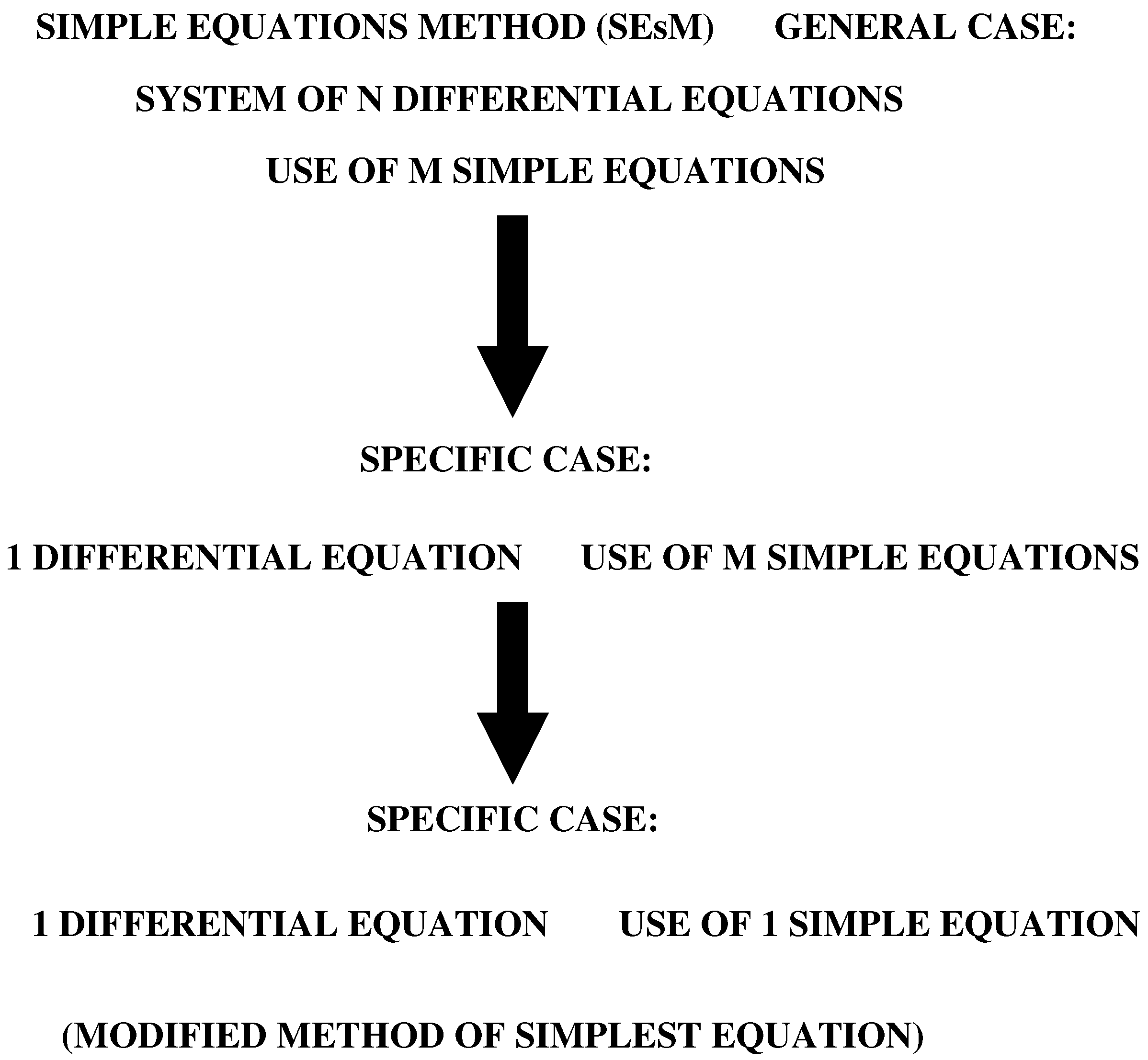
  • We developed a methodology for obtaining the exact and approximate solutions of nonlinear partial differential equations. The methodology is called the Simple Equations Method (SEsM) [47,48,49,50,51]. Some elements of the methodology can be seen in our publications written a long time ago [5253,54,55]. At the beginning [56,57], we used the ordinary differential equation of Bernoulli as the simplest equation [58]. This version of the methodology was called the Modified Method of the Simplest Equation (MMSE). It was used to obtain exact solutions of model nonlinear partial differential equations from ecology and population dynamics [59];
  • In these early publications, we used the concept of the balance equation. This helped us determine the kind of the simplest equations, as well as the form of the solution as a series of the solution of the simplest equation [60,61]. We note that the MMSE leads to results that are equivalent to the methodology of Kudryashov mentioned above. Our contributions to the methodology and its application till 2018 were connected to the MMSE [62,63,64,65,66,67]. We note especially the article [66]. It is connected to the part of the topics discussed below in the text;
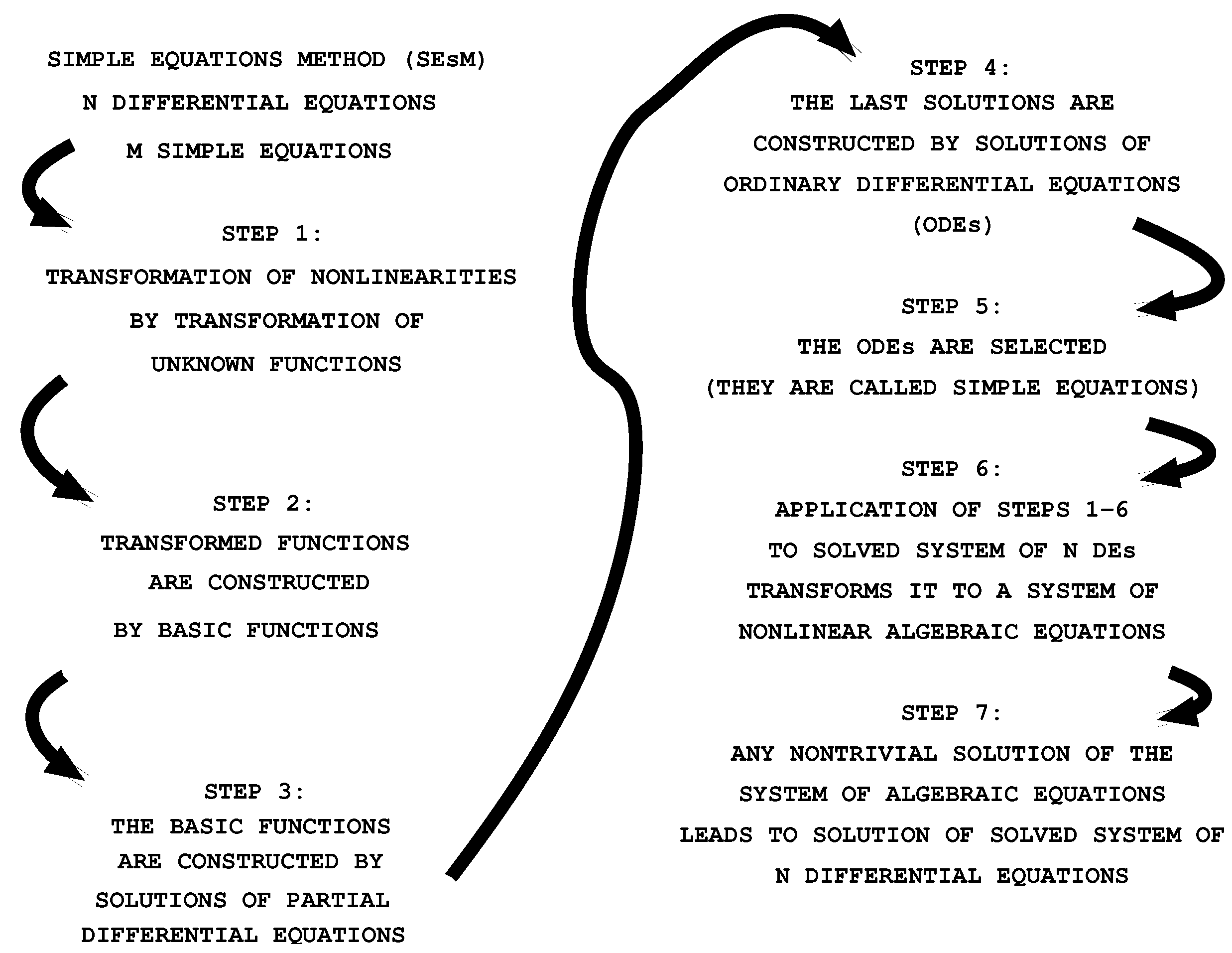
  • In the course of the years, the MMSE was extended to the SEsM [47]. The SEsM is connected to the possibility of the use of more than one simple equation. Thus, the solution of the solved nonlinear differential equation can be constructed on the basis of many simple equations. A version of the SEsM based on two simple equations was applied in [68]. The first description of the methodology was made in [48] and then in [47,49,50,51,69]. For more applications of specific cases of the SEsM, see [70,71,72].
Our idea in this study is as follows. We used the SEsM to study the mathematical problem for obtaining exact solutions of certain classes of nonlinear differential equations. Below, we were not interested in imposing boundary conditions on the solved differential equations. An important part of the SEsM is the construction of a solution of the solved equation. This solution is presented as a composite function of the solutions of simpler differential equations.
The text is organized as follows. We briefly describe the previous version of the SEsM from [47] in Section 2. Our interest below was to search for exact traveling wave solutions of one nonlinear differential equation. In Section 3, we discuss the amended version of the SEsM. It has a simplified schema because of the use of the composite function and its derivatives. One new theorem is discussed. In addition, a consequence of another theorem (proved by us) is considered. The theorem and the consequence are connected to the application of the SEsM to a specific case. This is the case of a nonlinear differential equation with polynomial nonlinearities and simple equations containing polynomial nonlinearities as well. Illustrative examples for the application of the amended version of the SEsM are discussed. Finally, several concluding remarks are given in Section 4.

2. Materials and Methods

Below, we discuss the simple equations method. It is an algorithm for obtaining exact and approximate solutions of nonlinear differential equations. The method was designed for the search of the solutions of systems of n nonlinear differential equations. The solution was constructed by the solutions of m simpler differential equations (Figure 1). The most applications of the algorithm up to now have been to obtain solutions of one nonlinear differential equation. This solution is searched as a function of the solution of one simple equation. The corresponding specific case of the SEsM is called the Modified Method of Simplest Equation (MMSE). Other kinds of examples exist as well. They present the solution of the solved nonlinear differential equation, which is a function of the solutions of several simple equations. Such examples can be seen in Section 3 below.
The version of the SEsM discussed in [47] has 7 steps. They are shown in Figure 2. We observed that this version of the methodology can be amended by the use of composite functions and their derivatives. The result was that the number of steps of the SEsM decreased from 7 to 4. This amended version is discussed below.

3. Results

3.1. The Amended Version of the SEsM

The amended version of the method of simple equations consists of four steps (see Figure 3). We unified Steps 2–4 from the previous version into Step 2 of the amended version. In addition, Steps 5 and 6 from the previous version were unified into Step 3 of the amended version. The description of the amended version of the methodology in is presented in more detail as follows.
We considered a system of nonlinear partial differential equations:
B i [ u 1 ( x , , t ) , , u n ( x , , t ) ] = 0 , i = 1 , , n .
In Equation (1), B i [ u 1 ( x , , t ) , , u n ( x , , t ) , ] depend on the functions u 1 ( x , , t ) , , u n ( x , , t ) and some of their derivatives ( u i can be a function of several spatial coordinates). We performed four steps:
(1)
We applied transformations:
u i ( x , . . . , t ) = T i [ F i ( x , , t ) , G i ( x , , t ) , ] .
T i ( F i , G i , ) is a function of other functions F i , G i , . F i ( x , , t ) , G i ( x , , t ) , … are functions of several spatial variables, as well as of time. The transformations T i have two goals:
(a)
They can remove some nonlinearities if possible (an example is the Hopf–Cole transformation, which leads to the linearization of the Burgers equation [20,21]);
(b)
They can transform the nonlinearity of the solved differential equations to a more treatable kind of nonlinearity (e.g., to polynomial nonlinearity).
In the case of one solved equation, the transformation T ( F , G , ) can be: the Painleve expansion; u ( x , t ) = 4 tan 1 [ F ( x , t ) ] in the case of the sine-Gordon equation; u ( x , t ) = 4 tanh 1 [ F ( x , t ) ] in the case of sh-Gordon (Poisson–Boltzmann equation) (for applications of the last two transformations, see, e.g., [52,53,54]); u ( x , t ) = F ( x , t ) G ( x , t ) ; u ( x , t ) = i = 0 I a i [ F ( x , t ) ] i j = 0 J b j [ G ( x , t ) ] j ; or another transformation.
In numerous cases, one may skip this step (then, we have u i ( x , , t ) = F i ( x , , t ) ). In many other cases, the transformation is needed to obtain a solution of the studied nonlinear PDE. The application of Equation (2) to Equation (1) leads to a nonlinear differential equations for the functions F i , G i , .
No general form is known for the transformations T i . The reason is that the nonlinearities in the solved equations can be of different kinds. The most studied cases of transformations are transformations that result in differential equations containing polynomial nonlinearities;
(2)
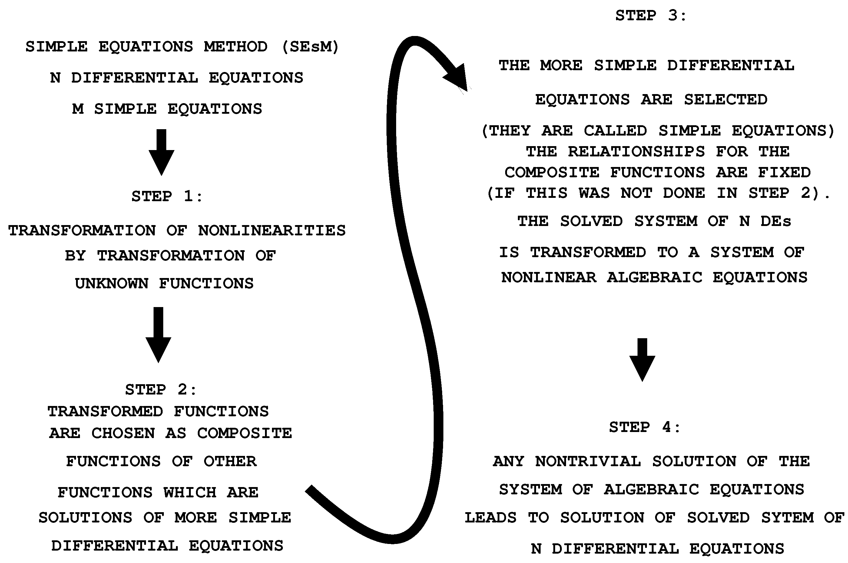
This step is based on the use of composite functions. It unifies Steps 2–4 from the version of the SEsM from [47]. In this step, the functions F i ( x , , t ) , G i ( x , , t ) , … are chosen as composite functions of the functions f i 1 , , f i N , g i 1 , , g i M , …, which are solutions of simpler differential equations (Step 2 in Figure 3). There are two possibilities:
(a)
The construction relationship for the composite function is not fixed. Then, we have to use the Faa di Bruno relationship for the derivatives of a composite function;
(b)
The construction relationship for the composite function is fixed. For example, for the case of one solved equation and one function F, the construction relationship can be chosen to be:
F = α + i 1 = 1 N β i 1 f i 1 + i 1 = 1 N i 2 = 1 N γ i 1 , i 2 f i 1 f i 2 + i 1 = 1 N i N = 1 N σ i 1 , , i N f i 1 f i N .
Then, one can directly calculate the corresponding derivatives from the solved differential equation;
(3)
In this step, we have to select the simple equations for the functions f i 1 , , f i N , g i 1 , , g i M , …. In addition, if we are in the hypothesis of Point (a) of Step 2, we have to fix the relationship between the composite functions F i ( x , , t ) , G i ( x , , t ) , …, and the functions f i 1 , , f i N , g i 1 , , g i M , …. We note that the fixation of the simple equations and the fixation of the relationships for the composite functions are connected. The fixations transform the left-hand sides of Equation (1). The result of this transformation can be functions that are the sum of terms. Each of these terms contains some function multiplied by a coefficient. This coefficient is a relationship containing some of the parameters of the solved equations and some of the parameters of the solutions of the simple equations used. The fixation mentioned above is performed by a balance procedure that ensures that the relationships for the coefficients contain more than one term. This balance procedure leads to one or more additional relationships among the parameters of the solved equation and parameters of the solutions of the simple equations used. These additional relationships are known as balance equations;
(4)
We may obtain a nontrivial solution of Equation (1) if all coefficients mentioned in Step 3 are set to zero. This condition usually leads to a system of nonlinear algebraic equations. The unknown variables in these equations are the coefficients of the solved nonlinear differential equation and the coefficients of the solutions of the simple equations. Any nontrivial solution of this algebraic system leads to a solution of the studied nonlinear partial differential equation.
From the system of algebraic equations, we determined the relationships for the parameters of the solution. Two possibilities exist:
(a)
The number, which is the sum of the number of parameters of the solution and the number of parameters of the equation, is larger than the number of algebraic equations or equal to the number of algebraic equations. Then, the system usually (but not in all of the cases) has a nontrivial solution (or solutions). Independent parameters may be presented in this solution. The other parameters of the solution are functions of the independent parameters;
(b)
The number, which is the sum of the number of parameters of the solution and the number of parameters of the equation, is smaller than the number of algebraic equations. Then, the system of algebraic equations usually does not have a nontrivial solution. However, there can be exceptions in this case. An exception occurs when the number of equations of the algebraic system can be reduced and this number becomes less than or equal to the number of available parameters. Then, Case (b) is reduced to Case (a), and a nontrivial solution is possible.

3.2. Faa di Bruno Relationship for Derivatives of a Composite Function

The composite functions play an important role in the amended version of the SEsM. Below, we provide information about the derivatives of the composite functions. These derivatives were used in the process of the application of the SEsM.

3.3. The General Case: Composite Function of Many Functions of Many Independent Variables

Let us consider the function h ( x 1 , , x d ) . It is a function of d independent variables x 1 , , x d . We assumed that the function h is a composite function of m other functions g 1 ( 1 ) , , g ( m ) :
h ( x 1 , , x d ) = f [ g ( 1 ) ( x 1 , , x d ) , , g ( m ) ( x 1 , , x d ) ] .
We introduce the following notations:
  • ν = ( ν 1 , , ν d ) is a d-dimensional index containing the integer non-negative numbers ν 1 , , ν d ;
  • z = ( z 1 , , z d ) is a d-dimensional object containing the real numbers z 1 , , z d ;
  • ν = i = 1 d ν i is the sum of the elements of the d-dimensional index ν ;
  • ν ! = i = 1 d ν i ! is the factorial of the multicomponent index ν ;
  • z ν = i = 1 d z i ν i is the ν -th power of the multicomponent variable z ;
  • D x ν = ν x 1 ν 1 x d ν d , ν > 0 is the ν -th derivative with respect to the multicomponent variable x . We note that in this notation, D x 0 is the identity operator;
  • z = max 1 i d z i is the maximum value component of the multicomponent variable z ;
  • For the d-dimensional index l = ( l 1 , , l d ) ( l 1 , , l d are integers), we have l ν when l i ν i , i = 1 , , d . Then, we define:
    ν l = i = 1 d ν i l i = ν ! l ! ( ν l ) ! ;
  • Ordering of vector indexes: For two vector indexes μ = ( μ 1 , , μ d ) and ν = ( ν 1 , , ν d ) , we have μ ν when one of the following holds:
    (a)
    μ < ν ;
    (b)
    μ = ν and μ 1 < ν 1 ;
    (c)
    μ = ν , μ 1 = ν 1 , … μ k = ν k and μ k + 1 < ν k + 1 for some 1 k < d .
Below, we also use the notation:
h ( ν ) = D x ν h ; f ( λ ) = D y λ f ; g ( μ ) ( i ) = D x μ g ( i ) ; g ( μ ) = ( g ( μ ) ( 1 ) , , g ( μ ) ( m ) ) .
Then, the Faa di Bruno relationship for the composite derivative of a function containing functions of many variables is [73]:
h ( ν ) = 1 λ n f ( λ ) s = 1 n p s ( ν , λ ) ( ν ! ) j = 1 s [ g ( l j ) ] k j ( k j ! ) [ l j ! ] k j .
In Equation (4), n = ν . In addition,
p s ( ν , λ ) = { k 1 , , k s ; l 1 , , l s } , k i > 0 .
Finally,
0 l 1 l s , i = 1 s k i = λ , i = 1 s k i l i = ν .
Equation (4) can be simplified by a change of the notation [73]. We introduce:
p ( ν , λ ) = { k 1 , , k n ; l 1 , , l n } , 1 s n .
In addition:
k i = 0 ; l i = 0 , 1 i n s , k i > 0 , n s + 1 i n .
Finally, 0 l n s + 1 l n are such that i = 1 n k i = λ i and i = 1 n k i l i = ν . Then, Equation (4) can be written as:
h ( ν ) = 1 λ n f ( λ ) p ( ν , λ ) ( ν ! ) j = 1 n [ g ( l j ) ] k j ( k j ! ) [ l j ! ] k j .

Several Specific Cases of the General Relationship

We discuss below the specific case when the composite function h is a function of two independent variables x 1 and x 2 . In this case:
h ( x 1 , x 2 ) = f [ g ( 1 ) ( x 1 , x 2 ) , , g ( m ) ( x 1 , x 2 ) ]
Then, from Equation (4), the Faa di Bruno formula for the composite function containing functions of two variables is:
h ( ν ) = ν 1 + ν 2 h x 1 ν 1 x 2 ν 2 = 1 ( λ 1 + + λ m ) ν 1 + ν 2 λ 1 + + λ m f g ( 1 ) λ 1 g ( m ) λ m { s = 1 ν 1 + ν 2 p s ( ν , λ ) ( ν 1 ! ν 2 ! ) × j = 1 s 1 ( k j , 1 ! k j , m ! ) ( l j , 1 ! + l j , 2 ! ) k j , 1 + + k j , m i = 1 m l j , 1 + l j , 2 x 1 l j , 1 x 2 l j , 2 g ( i ) k j , i } .
The version of the formula that arises from Equation (5) is:
h ( ν ) = ν 1 + ν 2 h x 1 ν 1 x 2 ν 2 = 1 ( λ 1 + + λ m ) ν 1 + ν 2 λ 1 + + λ m f g ( 1 ) λ 1 g ( m ) λ m { p ( ν , λ ) ( ν 1 ! ν 2 ! ) × j = 1 n 1 ( k j , 1 ! k j , m ! ) ( l j , 1 ! + l j , 2 ! ) k j , 1 + + k j , m i = 1 m l j , 1 + l j , 2 x 1 l j , 1 x 2 l j , 2 g ( i ) k j , i } .
Let us consider the case of the composite function containing three functions of two independent variables. In this case:
h ( x 1 , x 2 ) = f [ g ( 1 ) ( x 1 , x 2 ) , g ( 2 ) ( x 1 , x 2 ) , g ( 3 ) ( x 1 , x 2 ) ]
Then, from Equation (4), the Faa di Bruno formula for a composite function containing three functions of two independent variables is:
h ( ν ) = ν 1 + ν 2 h x 1 ν 1 x 2 ν 2 = 1 ( λ 1 + λ 2 + λ 3 ) ν 1 + ν 2 λ 1 + λ 2 + λ 3 f g ( 1 ) λ 1 g ( 2 ) λ 2 g ( 3 ) λ 3 { s = 1 ν 1 + ν 2 p s ( ν , λ ) ( ν 1 ! ν 2 ! ) × j = 1 s 1 ( k j , 1 ! k j , 2 ! k j , 3 ! ) ( l j , 1 ! + l j , 2 ! ) k j , 1 + k j , 2 + k j , 3 i = 1 3 l j , 1 + l j , 2 x 1 l j , 1 x 2 l j , 2 g ( i ) k j , i } .
The version of Equation (8) arising from Equation (5) is:
h ( ν ) = ν 1 + ν 2 h x 1 ν 1 x 2 ν 2 = 1 ( λ 1 + λ 2 + λ 3 ) ν 1 + ν 2 λ 1 + λ 2 + λ 3 f g ( 1 ) λ 1 g ( 2 ) λ 2 g ( 3 ) λ 3 { p ( ν , λ ) ( ν 1 ! ν 2 ! ) × j = 1 n 1 ( k j , 1 ! k j , 2 ! k j , 3 ! ) ( l j , 1 ! + l j , 2 ! ) k j , 1 + k j , 2 + k j , 3 i = 1 3 l j , 1 + l j , 2 x 1 l j , 1 x 2 l j , 2 g ( i ) k j , i } .
Next, we considered the case of the composite function containing two functions of two independent variables. In this case, the composite function is a function of the functions g ( 1 ) ( x 1 , x 2 ) and g ( 2 ) ( x 1 , x 2 ) . The Faa di Bruno formula for the composite function containing two functions that are functions of two variables is:
h ( ν ) = ν 1 + ν 2 h x 1 ν 1 x 2 ν 2 = 1 ( λ 1 + λ 2 ) ν 1 + ν 2 λ 1 + λ 2 f g ( 1 ) λ 1 g ( 2 ) λ 2 { s = 1 ν 1 + ν 2 p s ( ν , λ ) ( ν 1 ! ν 2 ! ) × j = 1 s 1 ( k j , 1 ! k j , 2 ! ) ( l j , 1 ! + l j , 2 ! ) k j , 1 + k j , 2 i = 1 2 l j , 1 + l j , 2 x 1 l j , 1 x 2 l j , 2 g ( i ) k j , i } .
The version of Equation (10) arising from Equation (5) is:
h ( ν ) = ν 1 + ν 2 h x 1 ν 1 x 2 ν 2 = 1 ( λ 1 + λ 2 ) ν 1 + ν 2 λ 1 + λ 2 f g ( 1 ) λ 1 g ( 2 ) λ 2 { p ( ν , λ ) ( ν 1 ! ν 2 ! ) × j = 1 n 1 ( k j , 1 ! k j , 2 ! ) ( l j , 1 ! + l j , 2 ! ) k j , 1 + k j , 2 i = 1 2 l j , 1 + l j , 2 x 1 l j , 1 x 2 l j , 2 g ( i ) k j , i } .
Finally, we considered the case of a composite function containing one function of one variable. For the case of one function of one variable h = f [ g ( x ) ] , the Faa di Bruno formula is:
h ( n ) = k = 1 n f ( k ) p ( k , n ) n ! i = 1 n g ( i ) λ i ( λ i ! ) ( i ! ) λ i .
In Equation (12):
  • h ( n ) = d n h d x n is the n-th derivative of the function h;
  • f ( k ) = d k f d g k is the k-th derivative of the function f;
  • g ( i ) = d i g d x i is the i-th derivative of the function g;
  • p ( n , k ) = { λ 1 , λ 2 , , λ n } : the set of numbers such that:
    i = 1 n λ i = k ; i = 1 n i λ i = n .

3.4. Several Results Relevant for Applications of the SEsM

Here, we present two theorems. They are for some features of the SEsM connected to the use of composite functions by this methodology. Theorem 1 is for the case of a differential equation containing polynomial nonlinearities where the unknown function h depends on two independent variables. The theorem states that for the case when the unknown function is a composite function, constructed by exponential functions, the solved equation can be reduced to a system of nonlinear algebraic equations. The theorem ensures that the SEsM is applicable in this case. The theorem is connected to the solutions of (1 + 1)-dimensional equations constructed on the basis of exponential functions. Many equations that have multisoliton solutions are of this class. The applicability of the discussed version of the SEsM to such equations is shown on the basis of a classic example—the Korteweg–de Vries equation. Another application is connected to obtaining standing wave solutions of differential equations for the case when these solutions are constructed by trigonometric and hyperbolic functions.
Theorem 2 shows that the SEsM can be applied also when the composite function is constructed by a function of a single variable and this function of a single variable satisfies the differential equation containing polynomial nonlinearities. We discuss a consequence of this theorem for the case when the simple equation used contains the equations of Bernoulli and Riccati as specific cases. This case ensures that the SEsM can be applied for the solution of differential equations containing polynomial nonlinearities for the cases when the simple equations used are the equations of Bernoulli, Riccati, Jacobi elliptic functions, etc. In such a way, we show why a large number of methods for obtaining exact solutions of nonlinear differential equations can be treated as specific cases of the SEsM.
Theorem 1.
Let us consider a nonlinear partial differential equation that contains a polynomial P of the function h ( x 1 , x 2 ) and its derivatives. The relationship for this equation is:
P ( h , h ν 1 , , h ν N ) = 0 .
Above, N can be any natural number. We searched for the solution of the above equation in the form:
h ( x 1 , x 2 ) = f [ g ( 1 ) ( x 1 , x 2 ) , , g ( m ) ( x 1 , x 2 ) ]
where h is the polynomial of the functions g ( 1 ) ( x 1 , x 2 ) , , g ( m ) ( x 1 , x 2 ) . Let each function g ( i ) ( x 1 , x 2 ) satisfy the simple equation:
g ( x j ) ( i ) = α i , j g ( i )
where α i , j is a constant parameter. Then, the solved nonlinear partial differential equation is reduced to a polynomial of the functions g ( 1 ) ( x 1 , x 2 ) , , g ( m ) ( x 1 , x 2 ) .
Proof. 
Let us consider Equation (7). We substituted Equation (2) in (7). The result is:
h ( ν ) = ν 1 + ν 2 h x 1 ν 1 x 2 ν 2 = 1 ( λ 1 + + λ m ) ν 1 + ν 2 λ 1 + + λ m f g ( 1 ) λ 1 g ( m ) λ m { p ( ν , λ ) ( ν 1 ! ν 2 ! ) × j = 1 n [ 1 ( k j , 1 ! k j , m ! ) ( l j , 1 ! + l j , 2 ! ) k j , 1 + + k j , m × α 1 , 1 l j , 1 k j , 1 α m , 1 l j , 1 k j , m α 1 , 2 l j , 2 k j , 1 α m , 2 l j , 2 k j , m g ( 1 ) k j , 1 g ( m ) k j , m ] } .
We looked at Equation (15). The term:
p ( ν , λ ) ( ν 1 ! ν 2 ! ) j = 1 n [ 1 ( k j , 1 ! k j , m ! ) ( l j , 1 ! + l j , 2 ! ) k j , 1 + + k j , m α 1 , 1 l j , 1 k j , 1 α m , 1 l j , 1 k j , m α 1 , 2 l j , 2 k j , 1 α m , 2 l j , 2 k j , m g ( 1 ) k j , 1 g ( m ) k j , m ] ,
is a polynomial of g ( 1 ) , , g ( m ) . It is multiplied by another polynomial of g ( 1 ) , , g ( m ) , namely by λ 1 + + λ m f g ( 1 ) λ 1 g ( m ) λ m . Thus, h ( ν ) is a polynomial of g ( 1 ) , , g ( m ) . Then, any of h ν 1 , , h ν N is a polynomial of g ( 1 ) , , g ( m ) . This means that P ( h , h ν 1 , , h ν N ) is a polynomial of g ( 1 ) , , g ( m ) . □
We note that the resulting polynomial P ( h , h ν 1 , , h ν N ) contains monomials multiplied by coefficients that are nonlinear algebraic relationships between the parameters of the solved nonlinear partial differential equation and parameters α i , j . We can set these coefficients to zero and obtain a system of nonlinear algebraic equations. Any nontrivial solution of this algebraic system (if such a solution exists) leads to a solution of the solved nonlinear partial differential Equation (13). Thus, Theorem 1 ensures that we can reduce to a nonlinear algebraic system any nonlinear differential equation that depends on two independent variables and has polynomial nonlinearities. In order to do this, we have to search for the solution as a composite function containing exponential functions. Theorem 1 is an indication of how to apply the SEsM in such cases. The class of equations concerned is a large one. Many important equations are in this class (e.g., many equations that have multisoliton solutions). For the convenience of the reader, we write the form of the derivatives of the composite function constructed by the exponential function for two cases. For the case of a composite function containing three exponential functions that are functions of two independent variables, we considered Equation (9) and substituted Equation (2) in (9). The result is:
h ( ν ) = ν 1 + ν 2 h x 1 ν 1 x 2 ν 2 = 1 ( λ 1 + λ 2 + λ 3 ) ν 1 + ν 2 λ 1 + λ 2 + λ 3 f g ( 1 ) λ 1 g ( 2 ) λ 2 g ( 3 ) λ 3 { p ( ν , λ ) ( ν 1 ! ν 2 ! ) × j = 1 n [ 1 ( k j , 1 ! k j , 2 ! k j , 3 ! ) ( l j , 1 ! + l j , 2 ! ) k j , 1 + k j , 2 + k j , 3 × α 1 , 1 l j , 1 k j , 1 α 2 , 1 l j , 1 k j , 2 α 3 , 1 l j , 1 k j , 3 α 1 , 2 l j , 2 k j , 1 α 2 , 2 l j , 2 k j , 2 α 3 , 2 l j , 2 k j , 3 g ( 1 ) k j , 1 g ( 2 ) k j , 2 g ( 3 ) k j , 3 ] } .
For the case of a composite function containing two exponential functions that are functions of two independent variables, we considered Equation (11). We substituted Equation (2) in (11). The result is:
h ( ν ) = ν 1 + ν 2 h x 1 ν 1 x 2 ν 2 = 1 ( λ 1 + λ 2 ) ν 1 + ν 2 λ 1 + λ 2 f g ( 1 ) λ 1 g ( 2 ) λ 2 { p ( ν , λ ) ( ν 1 ! ν 2 ! ) × j = 1 n [ 1 ( k j , 1 ! k j , 2 ! ) ( l j , 1 ! + l j , 2 ! ) k j , 1 + k j , 2 α 1 , 1 l j , 1 k j , 1 α 2 , 1 l j , 1 k j , 2 × α 1 , 2 l j , 2 k j , 1 α 2 , 2 l j , 2 k j , 2 g ( 1 ) k j , 1 g ( 2 ) k j , 2 ] } .
We can use simple equations that are more complicated than the equation for the exponential function (Equation (2)) in the SEsM. Let us consider the case of the composite function of one function, which depends on a single independent variable. Let us consider a nonlinear partial differential equation with nonlinearities that are polynomials of the unknown function h ( x , t ) and its derivatives. We searched for a solution of the kind:
h ( x , t ) = h ( ξ ) ; ξ = μ x + ν t ,
where μ and ν are parameters. The basis of our search is a solution g ( ξ ) of a certain simplest equation. Hence:
h = f [ g ( ξ ) ]
h from Equation (16) is a composite function. For the n-th derivative of h, we have the Faa di Bruno formula (12). Let us assume that f is a polynomial of g. Then:
f = r = 0 q b r g r .
We used the following simple equation:
g ( k ) l = d k g d ξ k l = j = 0 m a j g j .
In Equation (18), k , l , m are integers. The nonlinearity in Equation (18) is of the polynomial kind. As mentioned above, this simple equation is more complicated than Equation (2). The solution of Equation (18) defines the function V a 0 , a 1 , , a m ( ξ ; k , l , m ) where:
  • k: order of the derivative of g;
  • l: degree of the derivative in the defining ODE;
  • m: highest degree of the polynomial of g in the defining ODE.
This function V has interesting properties. Its specific cases are trigonometric, hyperbolic, elliptic functions of Jacobi, etc. Below, we used the function V a 0 , a 1 , , a m ( ξ ; 1 , 2 , m ) , which is the solution of the simple equation:
g ( 1 ) 2 = d g d ξ 2 = j = 0 m a j g j .
We have proven the following theorem [66].
Theorem 2.
If g ( 1 ) 2 is given by Equation (19) and f is a polynomial of g given by Equation (17), then for h [ f ( g ) ] , the following relationship holds:
h ( n ) = K n ( q , m ) ( g ) + g ( 1 ) Z n ( q , m ) ( g )
where K n ( q , m ) ( g ) and Z n ( q , m ) ( g ) are polynomials of the function g ( ξ ) .
The polynomials K n ( q , m ) ( g ) and Z n ( q , m ) ( g ) can be calculated as follows.
K 0 = r = 0 q b r g r Z 0 = 0
Then, starting from Equation (20), we obtain:
K n + 1 = Z n 2 j = 0 m j a j g j 1 + d Z n d g j = 0 m a j g j Z n + 1 = d K n d g .
Several of the polynomials K n and Z n from Equation (21) are calculated in Appendix A.
Theorem 2 can explain why many methods for obtaining exact traveling wave solutions of nonlinear partial differential equations that contain polynomial nonlinearities are specific cases of the SEsM. Many of these methods use simple equations, which are the equation of Bernoulli or the equation of Riccati. These equations are specific cases of Equation (19). This can be proven as follows. The equations of Bernoulli and Riccati are specific cases of the simple equation:
g ( 1 ) = j = 0 n c j g j .
In Equation (22), n and c j are constant parameters. However, Equation (22) is a specific case of (19). We prove this as follows. The idea is that Equation (19) contains all cases of (22). From Equation (22):
g ( 1 ) 2 = ( i = 0 n c i g i ) ( j = 0 n c j g j ) = i = 0 n j = 0 n c i c j g i + j = k = 0 2 n a k g k .
In Equation (23), a k are appropriate combinations of the coefficients c i . Equation (23) is of the kind (19). Then, Equation (19) contains all possible relationships of the kind (22). However, Equation (19) contains more than this. For example, Equation (19) contains the case:
g ( 1 ) 2 = a 0 + a 1 g .
Equation (24) cannot be reduced to a relationship of the kind (22). Then, Equation (22) is a specific case of (19).
Thus, the methods based on the use of the equations of Bernoulli and Riccati for the construction of solutions of nonlinear differential equations with polynomial nonlinearities are specific cases of the SEsM where the composite function can be represented according to Theorem 2. The discussed consequence of Theorem 2 shows, for example, that the homogeneous balance method [74] and tanh method [75] are specific cases of the SEsM.
The direct application of Theorem 2 is convenient when, for example, the simple equation is an equation for a Jacobi elliptic function. Theorem 2 shows that, for example, the Jacobi elliptic function expansion method [76] and the F-expansion method [77] are specific cases of the SEsM.
For the case when the simple equation has the specific form of Equation (22), we have a simpler situation. Instead of the two kinds of polynomials Z n and K n , we have a single kind of polynomial L n . In other words, for the case when the simple equation is of the kind (Equation (22)), h ( n ) is a polynomial of g: h ( n ) = L n ( g ) . These polynomials can be calculated as follows. We start from:
L 0 = r = 0 q b r g r .
Then, we use the recurrence relationship:
L i + 1 = d L i d g j = 0 m c j g j .
Several of the polynomials L i are calculated in Appendix B. In addition, we present in Appendix C several derivatives of a composite function that is function of two functions of two independent variables. In Appendix D, we present several derivatives of a composite function that is function of three functions of two independent variables. The information from these appendices are used in the examples below.

3.5. Illustrative Examples

The goal of the discussion below is to show how the methodology of the SEsM works. For an example, multisoliton solutions can be obtained. We show this for the Korteweg–de Vries equation. In addition, we show that the methodology can lead to specific solutions of nonlinear partial differential equations that are not integrable.
Below, we used the composite functions in the SEsM as follows. We used Equation (3) to fix the relationship for the composite function. On the basis of Equation (3), h can be written as:
h = T 0 + T 1 + + T N .
N can be any natural number. Note that the value of N can also be equal to . The relationships for T i are:
T 0 = α = const T 1 = i 1 = 1 N β i 1 g ( i 1 ) T 2 = i 1 = 1 N i 2 = 1 N γ i 1 , i 2 g ( i 1 ) g ( i 2 ) T 3 = i 1 = 1 N i 2 = 1 N i 3 = 1 N δ i 1 , i 2 , i 3 g ( i 1 ) g ( i 2 ) g ( i 3 ) T N = i 1 = 1 N i 2 = 1 N i N = 1 N σ i 1 , i 2 , , i N g ( i 1 ) g ( i 2 ) g ( i N )
We note that the functions g ( i n ) are the solutions of the corresponding simple equations. For the cases considered below, we used the following specific forms of Equations (26) and (27). For the case of the composite function of a function of one variable h = f [ g ( 1 ) ( ξ ) ] :
h = i = 0 N β i g ( 1 ) i .
In Equation (28), N is a parameter, which is fixed by means of balance equation.
For the case of the composite function of a function of two variables h = f [ g ( 1 ) ( x , t ) , g ( 2 ) ( x , t ) ] , we used the simple relationship:
h = α + β 1 g ( 1 ) + β 2 g ( 2 ) + γ 1 g ( 1 ) 2 + γ 2 g ( 2 ) 2 + γ 3 g ( 1 ) g ( 2 ) .
For the case of the composite function of a function of three variables h = f [ g ( 1 ) ( x , t ) , g ( 2 ) ( x , t ) , g ( 3 ) ( x , t ) ] , we used the simple relationship:
h = α + i = 1 3 β i g ( i 1 ) + i = 1 3 j = 1 3 γ i , j g ( i ) g ( j ) + i = 1 3 j = 1 3 k = 1 3 δ i , j , k g ( i ) g ( j ) g ( k ) .
Equations (28) and (29) were obtained by selecting only several terms from the large number of possible terms in Equation (26).
Next, we considered illustrative examples for the case of the composite function that is a function of one function of one variable. First of all, we considered the Korteweg–de Vries equation:
u t + 6 u u x + 3 u x 3 = 0 .
Following the steps of the SEsM, we applied the transformation:
u ( x , t ) = 2 2 x 2 [ ln h ( x , t ) ] = 2 h 2 h x 2 h x 2 h 2 .
This is Step 1 of the SEsM. The Korteweg–de Vries Equation (31) was transformed to:
h 2 h x t h x h t + h 4 h x 4 4 h x 3 h x 3 + 3 2 h x 2 2 = 0 .
Next, we considered h as a composite function of one function of one variable ξ = λ x + ω t + σ . λ , ω , and σ are parameters (Step 2 of the SEsM). Equation (33) was transformed to:
λ ω h d 2 h d ξ 2 λ ω d h d ξ 2 + λ 4 h d 4 h d ξ 4 4 λ 4 d h d ξ d 3 h d ξ 3 + 3 λ 4 d 2 h d ξ 2 2 = 0 .
In Step 3 of the SEsM, we used Equation (28) as the relationship for the composite function h. We set N = 1 in (28). In addition, the simple function g ( 1 ) ( ξ ) was assumed to satisfy the simple Equation (22) for the case n = 1 and c 0 = 0 . Then, the derivatives h ( n ) of the composite function h are given by the polynomials L i discussed above in the text (the relationships for L i are given in Appendix D).
In such a way, the Korteweg–de Vries Equation (34) was reduced to a polynomial that has to be equal to zero. This was achieved by setting the coefficients of the terms of the polynomial to zero. The result is a system of algebraic equations (Step 4 of the SEsM). This system of algebraic equations contains one equation:
ω + λ 3 c 1 2 = 0 ,
in addition to β 0 = 1 . Equation (35) can be solved for ω , for example. The solution is nontrivial. This, nontrivial solution leads to the one-soliton solution of the Korteweg–de Vries equation.
Another example is for the equation of the class:
p 1 h x + p 2 h 2 h x t + p 3 h 2 h x 2 + p 4 3 h x 3 + p 5 h 3 + p 6 h 2 + p 7 + p 8 = 0 .
In Equation (36), p 1 , p 2 , p 3 , p 4 , p 5 , p 6 , p 7 , p 8 are parameters. We skipped Step 1 of the SEsM (no transformation of the nonlinearity). In Step 2 of the SEsM, we used Equation (28) as the relationship for the composite function h. In Step 3 of the SEsM, we fixed the value of N. The form of the composite function h [ g ( 1 ) ( ξ ) ] ( ξ = α 1 x + α 2 t ) becomes:
h = β 2 g ( 1 ) 2 + β 1 g ( 1 ) + β 0 .
At the same time, the form of the simple equation for g ( 1 ) was fixed by means of a balance equation:
d g ( 1 ) d ξ = α g ( 1 ) 2 α g ( 1 ) .
By means of Equations (37) and (38), Equation (36) was reduced to a system of seven nonlinear algebraic equations (Step 4 of the SEsM). One nontrivial solution of this system is:
β 0 = 5 β 2 2 + 11 β 2 β 1 + 6 β 1 2 2 β 2 , A = 55 β 2 2 + 108 β 2 β 1 + 54 β 1 2 , B = 5 β 2 2 + 11 β 2 β 1 + 6 β 1 2 , C = 25 β 2 3 + 25 2 ( β 2 + β 1 ) B + 64 β 2 2 β 1 + 44 β 2 β 1 2 + 6 β 1 3 , p 1 = p 8 β 2 2 A 3 α α 1 B C , D = 95 β 2 3 + 126 β 1 3 + 317 β 2 2 β 1 + 348 β 2 β 1 2 30 ( β 2 + β 1 ) B , p 2 = 4 p 8 β 2 4 A B C D + p 3 α 2 α 1 2 α 2 α 1 α 2 , p 4 = 5 p 8 β 2 4 ( β 2 + β 1 ) A 3 α 3 α 1 3 B C D , p 5 = 24 p 8 β 2 3 A B C D , p 6 = 2 p 8 β 2 2 ( 97 β 2 2 + 198 β 2 β 1 + 99 β 1 2 ) A B C D , p 7 = 60 p 8 β 2 ( 17 β 2 2 + 36 β 2 β 1 + 18 β 1 2 ) ( 5 β 2 + 6 β 1 ) ( 175 β 2 3 + 528 β 2 2 β 1 + 513 β 2 β 1 2 + 162 β 1 3 ) .
The solution of the simple Equation (38) is:
g ( 1 ) ( ξ ) = 1 1 + exp ( α ξ ) .
Then, a particular exact solution of the equation:
p 8 β 2 2 A 3 α α 1 B C h x 4 p 8 β 2 4 A B C D + p 3 α 2 α 1 2 α 2 α 1 α 2 h 2 h x t + p 3 h 2 h x 2 5 p 8 β 2 4 ( β 2 + β 1 ) A 3 α 3 α 1 3 B C D 3 h x 3 + 24 p 8 β 2 3 A B C D h 3 2 p 8 β 2 2 ( 97 β 2 2 + 198 β 2 β 1 + 99 β 1 2 ) A B C D h 2 60 p 8 β 2 ( 17 β 2 2 + 36 β 2 β 1 + 18 β 1 2 ) ( 5 β 2 + 6 β 1 ) ( 175 β 2 3 + 528 β 2 2 β 1 + 513 β 2 β 1 2 + 162 β 1 3 ) + p 8 = 0 ,
is:
h ( ξ ) = β 2 1 1 + exp ( α ξ ) 2 + β 1 1 1 + exp ( α ξ ) + 5 β 2 2 + 11 β 2 β 1 + 6 β 1 2 2 β 2 ,
where:
ξ = α 1 x + α 2 t .
Next, we present examples for the case of the composite function that is a function of two functions of two variables. First, we considered again the Korteweg–de Vries equation. In this case, we applied the SEsM as follows. We used the transformation (32) and obtained Equation (33) from (31) (Step 1 of the SEsM). Then, we considered h as a composite functions of two functions of two variables. We used the relationship (29) (Step 2 of the SEsM). In addition, the simple functions g ( 1 ) ( η 1 ) and g ( 2 ) ( η 2 ) satisfy simple equations of the kind (22) for the case n = 1 and c 0 = 0 (Step 3 of the SEsM) η i = λ i x + ω i t + σ i , i = 1 , 2 . The further application of the methodology (Step 4 of the SEsM) led to γ 1 = γ 2 = 0 and reduced the Korteweg–de Vries equation to the system of two algebraic equations:
ω i + λ i 3 = 0 , i = 1 , 2 ,
in addition to α = 1 ; β 1 = β 2 = β , γ 3 = β 2 μ , where μ is a parameter. Equation (39) can be solved for ω i , i = 1 , 2 , for example. The solutions are nontrivial. These nontrivial solutions lead to the two-soliton solution of the Korteweg–de Vries equation.
Another example is connected to the equation:
( 1 + h 2 ) 2 h x 2 2 h t 2 2 h h x 2 h t 2 = h ( 1 h 2 ) .
We applied the SEsM and skipped Step 1 (no transformation of the nonlinearity). The composite function h is of the kind (29) where α = 0 , β 1 = β 2 = 0 , γ 1 = γ 2 = 0 (Step 2 of the SEsM). In addition, g ( 1 ) does not depend on t and g ( 2 ) does not depend on x. Let γ 3 = A . The composite function becomes:
h ( x , t ) = A g ( 1 ) ( α x ) g ( 2 ) ( δ γ t ) , δ = ± 1 .
We note that the composite function (41) allows for complicated simple equations for g ( 1 ) and g ( 2 ) . These equations can be of the kind of equations for the elliptic functions of Jacobi (Step 3 of the SEsM):
d g ( 1 ) d x 2 = α ( a 1 g ( 1 ) 4 + b 1 g ( 1 ) 2 + c 1 ) d g ( 2 ) d x 2 = β ( a 2 g ( 2 ) 4 + b 2 g ( 2 ) 2 + c 2 ) .
In Step 4 of the SEsM, Equation (40) is reduced to a system of algebraic equations:
α 2 b 1 γ 2 b 2 = 1 α 2 a 1 + γ 2 A 2 c 2 = 0 γ 2 a 2 + α 2 A 2 c 1 = 0 .
Equation (43) has various nontrivial solutions. For example, one of these solutions is when α 2 γ 2 < 1 . We can consider A as a free parameter. Then, α 2 = γ 2 + A 2 1 A 2 + 1 . Thus,
h ( x , t ) = A cn α x ; A 2 [ α 2 ( A 2 + 1 ) + 1 ] α 2 ( A 2 + 1 ) 2 cn δ γ t ; A 2 [ γ 2 ( A 2 + 1 ) 1 ] γ 2 ( A 2 + 1 ) 2 .
In Equation (44), cn ( α x ; k 1 ) and cn ( γ t ; k 2 ) are the corresponding Jacobi elliptic functions of modulus 0 k 1 1 and 0 k 2 1 , respectively.
Equation (43) has an interesting specific case when k 1 = 1 and k 1 = 0 . In this case, cn ( α x ; k 1 ) = sech ( α x ) and cn ( δ γ t ) = cos ( δ γ t ) . Then,
h ( x , t ) = cos δ ( A 2 + 1 ) 1 / 2 t cosh A 2 A 2 + 1 1 / 2 x .
Equation (45) can also be obtained straightforwardly on the basis of the composite function (41) if one takes for g ( 1 ) and g ( 2 ) the corresponding simple equations for the trigonometric and hyperbolic functions, respectively.
Finally, we discuss an example use case of the composite function that is a function of three functions of two variables. This led us to the three-soliton solution of the Korteweg–de Vries equation. In this case, we applied the SEsM as follows. We used the transformation (32) and obtained Equation (33) from (31). Then, we considered h as the composite function of three functions of two variables. We used the relationship (30). In addition, the simple functions g ( 1 ) ( η 1 ) , g ( 2 ) ( η 2 ) , and g ( 3 ) ( η 3 ) satisfy simple equations of the kind of Equation (22) for the case n = 1 and c 0 = 0 . η i = λ i x + ω i t + σ i , i = 1 , 2 , 3 . The application of the SEsM led to γ 1 = γ 2 = 0 and reduced the Korteweg–de Vries equation to the system of three algebraic equations:
ω i + λ i 3 = 0 , i = 1 , 2 , 3 ,
in addition to α = 1 ; β 1 = β 2 = β 3 = β , γ i , i = 0 , δ i , j , k = 0 except for δ 1 , 2 , 3 . Moreover, γ i , j = β a i , j where a i , j = ( λ i λ j ) 2 ( λ i + λ j ) 2 , i , j = 1 , 2 , 3 , i < j . Finally, δ 1 , 2 , 3 = β a 1 , 2 a 1 , 3 a 2 , 3 .
Equation (46) can be solved for ω i , i = 1 , 2 , 3 , for example. The solutions are nontrivial. These nontrivial solutions led to the three-soliton solution of the Korteweg–de Vries equation.

4. Concluding Remarks

This article was devoted to a discussion of the methodology called the Simple Equations Method (SEsM) and several results connected to this methodology. The new results were as follows:
  • We presented an amended version of the SEsM in comparison to the version from [47]. The amended version was based on the use of composite functions and their derivatives. In such a way, the number of steps of the SEsM was reduced from seven to four. In the amended version of the SEsM, we determined the form of the composite functions used. This increased the amount of computations with respect to the amount of computations for the version of the SEsM with seven steps. In the last version, we made assumptions about the form of the relationships among the solutions of the solved equations and the solutions of the simple equations. This led to the intermediate steps, but decreased the amount of computation. However, if the assumptions are not appropriate, we may miss the solutions of the solved equations;
  • We discussed a theorem that states that under certain conditions, a nonlinear differential equation with polynomials nonlinearities can be reduced to a polynomial containing monomials consisting of exponential functions. This theorem justified the application of the SEsM as the setting of the coefficients of the obtained polynomial to zero led to a system of nonlinear algebraic equation, which led exactly to Step 4 of the SEsM. We note that in such a way, the SEsM can lead to multisoliton solutions of a large class of equations. An illustrative example for the Korteweg–de Vries equation was given;
  • A consequence of a theorem proven in [66] was used in order to show that the simple equation of the SEsM can contain polynomial nonlinearities of large power for the case when the composite function used in the SEsM is a function of one independent variable. This consequence showed that many methods that search for exact traveling wave solutions of nonlinear differential equations on the basis, for example, of the equations of Riccati and Bernoulli are specific cases of the SEsM;
  • We presented many illustrative examples for the application of the amended version of the SEsM.
Finally, we want to stress that the SEsM is an interesting methodology for obtaining exact solutions of nonlinear differential equations. We showed already that the SEsM is connected to the inverse scattering transform method and to the method of Hirota [47]. The SEsM can lead to specific solutions also of nonintegrable differential equations. The use of composite functions in the methodology of the SEsM opens possibilities for obtaining additional results on the methodology, as well as specific solutions of many nonlinear differential equations. In addition, the kinds of nonlinearities different from polynomial ones can be treated. This will be one of the goals of our future research.

Author Contributions

Conceptualization, N.K.V. and Z.I.D.; methodology, N.K.V.; software, K.N.V.; validation, Z.I.D. and K.N.V.; formal analysis, N.K.V., Z.I.D., and K.N.V.; resources, N.K.V.; data curation, Z.I.D. and K.N.V.; writing—original draft preparation, N.K.V., Z.I.D., and K.N.V.; writing—review and editing, N.K.V.; visualization, K.N.V.; supervision, N.K.V. and Z.I.D.; project administration, Z.I.D. and K.N.V.; funding acquisition, N.K.V. All authors have read and agreed to the published version of the manuscript.

Funding

This research was partially supported by the project BG05 M2OP001-1.001-0008 “National Center for Mechatronics and Clean Technologies”, funded by the Operating Program “Science and Education for Intelligent Growth” of Republic of Bulgaria and by the National Scientific Program “Information and Communication Technologies for a Single Digital Market in Science, Education and Security” (ICTinSES), Contract No. D01205/23.11.2018, financed by the Ministry of Education and Science in Bulgaria.

Institutional Review Board Statement

Not applicable.

Informed Consent Statement

Not applicable.

Data Availability Statement

Not applicable.

Conflicts of Interest

The authors declare no conflict of interest.

Appendix A. Several Polynomials Kn and Zn

The derivatives h ( 1 ) , h ( 2 ) , h ( 3 ) , h ( 4 ) , h ( 5 ) , h ( 6 ) , and h ( 7 ) are often used in the model nonlinear partial differential equations. Below, we calculated the polynomials K n and Z n connected to these derivatives. We start from:
K 0 = r = 0 q b r g r Z 0 = 0
From Equation (21), we obtain:
K 1 = 0 ; Z 1 = r = 0 q r b r g r 1
Then:
K 2 = r = 0 q j = 0 m 1 2 j r + r ( r 1 ) a j b r g j + r 2 Z 2 = 0 .
K 3 = 0 ; Z 3 = r = 0 q j = 0 m 1 2 j r + r ( r 1 ) ( j + r 2 ) a j b r g j + r 3
K 4 = r = 0 q j = 0 m u = 0 m 1 2 j r + r ( r 1 ) ( j + r 2 ) 1 2 u + j + r 3 a j b r a u g j + r + u 4 Z 4 = 0 .
K 5 = 0 ; Z 5 = r = 0 q j = 0 m u = 0 m 1 2 j r + r ( r 1 ) ( j + r 2 ) 1 2 u + j + r 3 ( j + r + u 4 ) a j b r a u g j + r + u 5
K 6 = r = 0 q j = 0 m u = 0 m v = 0 m [ 1 2 j r + r ( r 1 ) ( j + r 2 ) 1 2 u + j + r 3 ( j + r + u 4 ) ] 1 2 v + j + r + u 5 a j b r a u a v g j + r + u + v 6 Z 6 = 0 .
K 7 = 0 ; Z 7 = r = 0 q j = 0 m u = 0 m v = 0 m [ 1 2 j r + r ( r 1 ) ( j + r 2 ) 1 2 u + j + r 3 ( j + r + u 4 ) ] 1 2 v + j + r + u 5 ( j + r + u + v 6 ) a j b r a u a v g j + r + u + v 7 ,
etc.

Appendix B. Polynomials Li

We write below several of the polynomials L i for the case (22) We start from:
L 0 = r = 0 q b r g r .
The application of the recurrence relationship (25) leads to the following relationships for L 1 , L 2 , ….
L 1 = r = 0 q j = 0 m b r r c j g r + j 1 .
L 2 = r = 0 q j = 0 m k = 0 m b r r ( r + j 1 ) c j c k g r + j + k 2 .
L 3 = r = 0 q j = 0 m k = 0 m l = 0 m b r r ( r + j 1 ) ( r + j + k 2 ) c j c k c l g r + j + k + l 3 .
L 4 = r = 0 q j = 0 m k = 0 m l = 0 m n = 0 m b r r ( r + j 1 ) ( r + j + k 2 ) ( r + j + k + l 3 ) c j c k c l c n × g r + j + k + l + n 4 .
L 5 = r = 0 q j = 0 m k = 0 m l = 0 m n = 0 m p = 0 m b r r ( r + j 1 ) ( r + j + k 2 ) ( r + j + k + l 3 ) × ( r + j + k + l + n 4 ) c j c k c l c n c p g r + j + k + l + n + p 5 .
L 6 = r = 0 q j = 0 m k = 0 m l = 0 m n = 0 m p = 0 m u = 0 m b r r ( r + j 1 ) ( r + j + k 2 ) ( r + j + k + l 3 ) × ( r + j + k + l + n 4 ) ( r + j + k + l + n + p 5 ) c j c k c l c n c p c u g r + j + k + l + n + p + u 6 .
L 7 = r = 0 q j = 0 m k = 0 m l = 0 m n = 0 m p = 0 m u = 0 m v = 0 m b r r ( r + j 1 ) ( r + j + k 2 ) ( r + j + k + l 3 ) × ( r + j + k + l + n 4 ) ( r + j + k + l + n + p 5 ) ( r + j + k + l + n + p + u 6 ) × c j c k c l c n c p c u c v g r + j + k + l + n + p + u + v 7 .

Appendix C. Several Derivatives for the Case of a Function That Is a Composite Function of Two Functions of Two Independent Variables

In this case, h = f [ g ( 1 ) ( x , t ) , g ( 2 ) ( x , t ) ] . The derivatives up to order three are as follows:
h x = f g ( 1 ) g ( 1 ) x + f g ( 2 ) g ( 2 ) x ,
h t = f g ( 1 ) g ( 1 ) t + f g ( 2 ) g ( 2 ) t .
2 h x 2 = 2 f g ( 1 ) 2 g ( 1 ) x 2 + 2 2 f g ( 1 ) g ( 2 ) g ( 1 ) x g ( 2 ) x + f g ( 1 ) 2 g ( 1 ) x 2 + 2 f g ( 2 ) 2 g ( 2 ) x 2 + f g ( 2 ) 2 g ( 2 ) x 2 .
2 h t 2 = 2 f g ( 1 ) 2 g ( 1 ) t 2 + 2 2 f g ( 1 ) g ( 2 ) g ( 1 ) t g ( 2 ) t + f g ( 1 ) 2 g ( 1 ) t 2 + 2 f g ( 2 ) 2 g ( 2 ) t 2 + f g ( 2 ) 2 g ( 2 ) t 2 .
2 h x t = 2 f g ( 1 ) 2 g ( 1 ) x g ( 1 ) t + 2 f g ( 1 ) g ( 2 ) g ( 1 ) x g ( 2 ) t + f g ( 1 ) 2 g ( 1 ) x t + 2 f g ( 1 ) g ( 2 ) g ( 1 ) t g ( 2 ) x + 2 f g ( 2 ) 2 g ( 2 ) x g ( 2 ) t + f g ( 2 ) 2 g ( 2 ) x t .
h x 3 = 3 f g ( 1 ) 3 g ( 1 ) x 3 + 3 3 f g ( 1 ) 2 g ( 2 ) g ( 1 ) x 2 g ( 2 ) x + 3 2 f g ( 1 ) 2 g ( 1 ) x 2 g ( 1 ) x 2 + 3 2 f g ( 1 ) g ( 2 ) 2 g ( 1 ) x 2 g ( 2 ) x + 3 3 f g ( 1 ) g ( 2 ) 2 g ( 1 ) x g ( 2 ) x 2 + 3 2 f g ( 1 ) g ( 2 ) g ( 1 ) x 2 g ( 2 ) x 2 + f g ( 1 ) 3 g ( 1 ) x 3 + 3 f g ( 2 ) 3 g ( 2 ) x 3 + 3 2 f g ( 2 ) 2 g ( 2 ) x 2 g ( 2 ) x 2 + f g ( 2 ) 3 g ( 2 ) x 3 .
h t 3 = 3 f g ( 1 ) 3 g ( 1 ) t 3 + 3 3 f g ( 1 ) 2 g ( 2 ) g ( 1 ) t 2 g ( 2 ) t + 3 2 f g ( 1 ) 2 g ( 1 ) t 2 g ( 1 ) t 2 + 3 2 f g ( 1 ) g ( 2 ) 2 g ( 1 ) t 2 g ( 2 ) t + 3 3 f g ( 1 ) g ( 2 ) 2 g ( 1 ) t g ( 2 ) t 2 + 3 2 f g ( 1 ) g ( 2 ) g ( 1 ) t 2 g ( 2 ) t 2 + f g ( 1 ) 3 g ( 1 ) t 3 + 3 f g ( 2 ) 3 g ( 2 ) t 3 + 3 2 f g ( 2 ) 2 g ( 2 ) t 2 g ( 2 ) t 2 + f g ( 2 ) 3 g ( 2 ) t 3 .
h x 2 t = 3 f g ( 1 ) 3 g ( 1 ) x 2 g ( 1 ) t + 3 f g ( 1 ) 2 g ( 2 ) g ( 1 ) x 2 g ( 2 ) t + 2 2 f g ( 1 ) 2 g ( 1 ) x 2 g ( 1 ) x t + 2 2 f g ( 1 ) g ( 2 ) 2 g ( 1 ) x t g ( 2 ) x + 2 3 f g ( 1 ) 2 g ( 2 ) g ( 1 ) x g ( 2 ) x g ( 1 ) t + 2 3 f g ( 1 ) g ( 2 ) 2 g ( 1 ) x g ( 2 ) x g ( 2 ) t + 2 2 f g ( 1 ) g ( 2 ) g ( 1 ) x 2 g ( 2 ) x t + 2 f g ( 1 ) 2 2 g ( 1 ) x 2 g ( 1 ) t + 2 f g ( 1 ) g ( 2 ) 2 g ( 1 ) x 2 g ( 2 ) t + f g ( 1 ) 3 g ( 1 ) x 2 t + 3 f g ( 1 ) g ( 2 ) 2 g ( 2 ) x 2 g ( 1 ) t + 3 f g ( 2 ) 3 g ( 2 ) x 2 g ( 2 ) t + 2 2 f g ( 2 ) 2 g ( 2 ) x 2 g ( 2 ) x t + 2 f g ( 1 ) g ( 2 ) 2 g ( 2 ) x 2 g ( 1 ) t + 2 f g ( 2 ) 2 2 g ( 2 ) x 2 g ( 2 ) t + f g ( 2 ) 3 g ( 2 ) x 2 t .
h x t 2 = 3 f g ( 1 ) 3 g ( 1 ) x g ( 1 ) t 2 + 2 2 f g ( 1 ) 2 2 g ( 1 ) x t g ( 1 ) t + 2 3 f g ( 1 ) 2 g ( 2 ) g ( 1 ) x g ( 1 ) t g ( 2 ) t + 2 f g ( 1 ) 2 g ( 1 ) x 2 g ( 1 ) t 2 + 2 2 f g ( 1 ) g ( 2 ) g ( 1 ) x t g ( 2 ) t + 3 f g ( 1 ) g ( 2 ) 2 g ( 1 ) x g ( 2 ) t 2 + 2 f g ( 1 ) g ( 2 ) g ( 1 ) x 2 g ( 2 ) t 2 + f g ( 1 ) 3 g ( 1 ) x t 2 + 2 2 f g ( 1 ) g ( 2 ) 2 g ( 2 ) x t g ( 1 ) t + 3 f g ( 1 ) 2 g ( 2 ) g ( 2 ) x g ( 1 ) t 2 + 2 3 f g ( 1 ) g ( 2 ) 2 g ( 2 ) x g ( 1 ) t g ( 2 ) t + 2 f g ( 1 ) g ( 2 ) g ( 2 ) x 2 g ( 1 ) t 2 + 2 2 f g ( 2 ) 2 2 g ( 2 ) x t g ( 2 ) t + 3 f g ( 2 ) 3 g ( 2 ) x g ( 2 ) t 2 + 2 f g ( 2 ) 2 g ( 2 ) x 2 g ( 2 ) t 2 + f g ( 2 ) 3 g ( 2 ) x t 2 .
We considered the specific case:
g ( i ) x j = α i , j g ( i ) ,
where x 1 = x and x 2 = t . For this case, the above relationships are as follows:
h x = α 1 , 1 g ( 1 ) f g ( 1 ) + α 2 , 1 g ( 2 ) f g ( 2 ) ,
h t = α 1 , 2 g ( 1 ) f g ( 1 ) + α 2 , 2 g ( 2 ) f g ( 2 ) .
2 h x 2 = α 1 , 1 2 g ( 1 ) 2 2 f g ( 1 ) 2 + 2 α 1 , 1 α 2 , 1 g ( 1 ) g ( 2 ) 2 f g ( 1 ) g ( 2 ) + α 1 , 1 2 g ( 1 ) f g ( 1 ) + α 2 , 1 2 g ( 2 ) 2 2 f g ( 2 ) 2 + α 2 , 1 2 g ( 2 ) f g ( 2 ) .
2 h t 2 = α 1 , 2 2 g ( 1 ) 2 2 f g ( 1 ) 2 + 2 α 1 , 2 α 2 , 2 g ( 1 ) g ( 2 ) 2 f g ( 1 ) g ( 2 ) + α 1 , 2 2 g ( 1 ) f g ( 1 ) + α 2 , 2 2 g ( 2 ) 2 2 f g ( 2 ) 2 + α 2 , 2 2 g ( 2 ) f g ( 2 ) .
2 h x t = α 1 , 1 α 1 , 2 g ( 1 ) 2 2 f g ( 1 ) 2 + α 1 , 1 α 2 , 2 g ( 1 ) g ( 2 ) 2 f g ( 1 ) g ( 2 ) + α 1 , 1 α 1 , 2 g ( 1 ) f g ( 1 ) + α 1 , 2 α 2 , 1 g ( 1 ) g ( 2 ) 2 f g ( 1 ) g ( 2 ) + α 2 , 1 α 2 , 2 g ( 2 ) 2 2 f g ( 2 ) 2 + α 2 , 1 α 2 , 2 g ( 2 ) f g ( 2 ) .
h x 3 = α 1 , 1 3 g ( 1 ) 2 3 f g ( 1 ) 3 + 3 α 1 , 1 2 α 2 , 1 g ( 1 ) 2 g ( 2 ) 3 f g ( 1 ) 2 g ( 2 ) + 3 α 1 , 1 3 g ( 1 ) 2 2 f g ( 1 ) 2 + 3 α 1 , 1 2 α 2 , 1 g ( 1 ) g ( 2 ) 2 f g ( 1 ) g ( 2 ) + 3 α 1 , 1 α 2 , 1 2 g ( 1 ) g ( 2 ) 2 3 f g ( 1 ) g ( 2 ) 2 + 3 α 1 , 1 α 2 , 1 2 g ( 1 ) g ( 2 ) 2 f g ( 1 ) g ( 2 ) + α 1 , 1 3 g ( 1 ) f g ( 1 ) + α 2 , 1 3 g ( 2 ) 3 3 f g ( 2 ) 3 + 3 α 2 , 1 3 g ( 2 ) 2 2 f g ( 2 ) 2 + α 2 , 1 3 g ( 2 ) f g ( 2 ) .
h t 3 = α 1 , 2 3 g ( 1 ) 3 3 f g ( 1 ) 3 + 3 α 1 , 2 2 α 2 , 2 g ( 1 ) 2 g ( 2 ) 3 f g ( 1 ) 2 g ( 2 ) + 3 α 1 , 2 3 g ( 1 ) 2 2 f g ( 1 ) 2 + 3 α 1 , 2 2 α 2 , 2 g ( 1 ) g ( 2 ) 2 f g ( 1 ) g ( 2 ) + 3 α 1 , 2 α 2 , 2 2 g ( 1 ) g ( 2 ) 2 3 f g ( 1 ) g ( 2 ) 2 + 3 α 1 , 2 α 2 , 2 2 g ( 1 ) g ( 2 ) 2 f g ( 1 ) g ( 2 ) + α 1 , 2 3 g ( 1 ) f g ( 1 ) + α 2 , 2 3 g ( 2 ) 3 3 f g ( 2 ) 3 + 3 α 2 , 2 3 g ( 2 ) 2 2 f g ( 2 ) 2 + α 2 , 2 3 g ( 2 ) f g ( 2 ) .
h x 2 t = α 1 , 1 2 α 1 , 2 g ( 1 ) 3 3 f g ( 1 ) 3 + α 1 , 1 2 α 2 , 2 g ( 1 ) 2 g ( 2 ) 3 f g ( 1 ) 2 g ( 2 ) + 2 α 1 , 1 2 α 1 , 2 g ( 1 ) 2 2 f g ( 1 ) 2 + 2 α 1 , 1 α 1 , 2 α 2 , 1 g ( 1 ) g ( 2 ) 2 f g ( 1 ) g ( 2 ) + 2 α 1 , 1 α 2 , 1 α 1 , 2 g ( 1 ) 2 g ( 2 ) 3 f g ( 1 ) 2 g ( 2 ) + 2 α 1 , 1 α 2 , 1 α 2 , 2 g ( 1 ) g ( 2 ) 2 3 f g ( 1 ) g ( 2 ) 2 + 2 α 1 , 1 α 2 , 1 α 2 , 2 g ( 1 ) g ( 2 ) 2 f g ( 1 ) g ( 2 ) + α 1 , 1 2 α 1 , 2 g ( 1 ) 2 2 f g ( 1 ) 2 + α 1 , 1 2 α 2 , 2 g ( 1 ) g ( 2 ) 2 f g ( 1 ) g ( 2 ) + α 1 , 1 2 α 1 , 2 g ( 1 ) f g ( 1 ) + α 2 , 1 2 α 1 , 2 g ( 1 ) g ( 2 ) 2 3 f g ( 1 ) g ( 2 ) 2 + α 2 , 1 2 α 2 , 2 g ( 2 ) 3 3 f g ( 2 ) 3 + 2 α 2 , 1 2 α 2 , 2 g ( 2 ) 2 2 f g ( 2 ) 2 + α 2 , 1 2 α 1 , 2 g ( 1 ) g ( 2 ) 2 f g ( 1 ) g ( 2 ) + α 2 , 1 2 α 2 , 2 g ( 2 ) 2 2 f g ( 2 ) 2 + α 2 , 1 2 α 2 , 2 g ( 2 ) f g ( 2 ) .
h x t 2 = α 1 , 1 α 1 , 2 2 g ( 1 ) 3 3 f g ( 1 ) 3 + 2 α 1 , 1 α 1 , 2 2 g ( 1 ) 2 2 f g ( 1 ) 2 + 2 α 1 , 1 α 1 , 2 α 2 , 2 g ( 1 ) 2 g ( 2 ) 3 f g ( 1 ) 2 g ( 2 ) + α 1 , 1 α 1 , 2 2 g ( 1 ) 2 2 f g ( 1 ) 2 + 2 α 1 , 2 α 1 , 2 α 2 , 1 g ( 1 ) g ( 2 ) 2 f g ( 1 ) g ( 2 ) + α 1 , 1 α 2 , 2 2 g ( 1 ) g ( 2 ) 2 3 f g ( 1 ) g ( 2 ) 2 + α 1 , 1 α 2 , 2 2 g ( 1 ) g ( 2 ) 2 f g ( 1 ) g ( 2 ) + α 1 , 1 α 1 , 2 2 g ( 1 ) f g ( 1 ) + 2 α 1 , 2 α 2 , 1 α 2 , 2 g ( 1 ) g ( 2 ) 2 f g ( 1 ) g ( 2 ) + α 2 , 1 α 1 , 2 2 g ( 1 ) 2 g ( 2 ) 3 f g ( 1 ) 2 g ( 2 ) + 2 α 1 , 2 α 2 , 1 α 2 , 2 g ( 1 ) g ( 2 ) 2 3 f g ( 1 ) g ( 2 ) 2 + α 2 , 1 α 1 , 2 2 g ( 1 ) g ( 2 ) 2 f g ( 1 ) g ( 2 ) + 2 α 2 , 1 α 2 , 2 2 g ( 2 ) 2 2 f g ( 2 ) 2 + α 2 , 1 α 2 , 2 2 g ( 2 ) 3 3 f g ( 2 ) 3 + α 2 , 1 α 2 , 2 2 g ( 2 ) 2 2 f g ( 2 ) 2 + α 2 , 1 α 2 , 2 2 g ( 2 ) f g ( 2 ) .

Appendix D. Several Derivatives for the Case of a Function That Is a Composite Function of Three Functions of Two Independent Variables

In this case, h = f [ g ( 1 ) ( x , t ) , g ( 2 ) ( x , t ) , g ( 3 ( x , t ) ] . The derivatives up to order two are as follows:
h x = f g ( 1 ) g ( 1 ) x + f g ( 2 ) g ( 2 ) x + f g ( 3 ) g ( 3 ) x ,
h t = f g ( 1 ) g ( 1 ) t + f g ( 2 ) g ( 2 ) t + f g ( 3 ) g ( 3 ) t .
2 h x 2 = 2 f g ( 1 ) 2 g ( 1 ) x 2 + 2 2 f g ( 1 ) g ( 2 ) g ( 1 ) x g ( 2 ) x + 2 2 f g ( 1 ) g ( 3 ) g ( 1 ) x g ( 3 ) x + f g ( 1 ) 2 g ( 1 ) x 2 + 2 f g ( 2 ) 2 g ( 2 ) x 2 + 2 2 f g ( 2 ) g ( 3 ) g ( 2 ) x g ( 3 ) x + f g ( 2 ) 2 g ( 2 ) x 2 + 2 f g ( 3 ) 2 g 3 x 2 + f g ( 3 ) 2 g ( 3 ) x 2 .
2 h t 2 = 2 f g ( 1 ) 2 g ( 1 ) t 2 + 2 2 f g ( 1 ) g ( 2 ) g ( 1 ) t g ( 2 ) t + 2 2 f g ( 1 ) g ( 3 ) g ( 1 ) t g ( 3 ) t + f g ( 1 ) 2 g ( 1 ) t 2 + 2 f g ( 2 ) 2 g ( 2 ) t 2 + 2 2 f g ( 2 ) g ( 3 ) g ( 2 ) t g ( 3 ) t + f g ( 2 ) 2 g ( 2 ) t 2 + 2 f g ( 3 ) 2 g 3 t 2 + f g ( 3 ) 2 g ( 3 ) t 2 .
2 h x t = 2 f g ( 1 ) 2 g ( 1 ) x g ( 1 ) t + 2 f g ( 1 ) g ( 2 ) g ( 1 ) x g ( 2 ) t + 2 f g ( 1 ) g ( 3 ) g ( 1 ) x g ( 3 ) t + f g ( 1 ) 2 g ( 1 ) x t + 2 f g ( 1 ) g ( 2 ) g ( 2 ) x g ( 1 ) t + 2 f g ( 2 ) 2 g ( 2 ) x g ( 2 ) t + 2 f g ( 2 ) g ( 3 ) g ( 2 ) x g ( 3 ) t + f g ( 2 ) 2 g ( 2 ) x t + 2 f g ( 1 ) g ( 3 ) g ( 3 ) x g ( 1 ) t + 2 f g ( 2 ) g ( 3 ) g ( 2 ) t g ( 3 ) x + 2 f g ( 3 ) 2 g ( 3 ) x g ( 3 ) t + f g ( 3 ) 2 g ( 3 ) x t .
We considered the specific case:
g ( i ) x j = α i , j g ( i ) ,
where x 1 = x and x 2 = t . For this case, the above relationships are as follows:
h x = α 1 , 1 f g ( 1 ) + α 2 , 1 f g ( 2 ) + α 3 , 1 f g ( 3 ) ,
h t = α 1 , 2 f g ( 1 ) + α 2 , 2 f g ( 2 ) + α 3 , 2 f g ( 3 ) .
2 h x 2 = α 1 , 1 2 g ( 1 ) 2 2 f g ( 1 ) 2 + 2 α 1 , 1 α 2 , 1 g ( 1 ) g ( 2 ) 2 f g ( 1 ) + 2 α 1 , 1 α 3 , 1 g ( 1 ) g ( 3 ) 2 f g ( 1 ) g ( 3 ) + α 1 , 1 2 g ( 1 ) f g ( 1 ) + α 2 , 1 2 g ( 2 ) 2 2 f g ( 2 ) 2 + 2 α 2 , 1 α 3 , 1 g ( 2 ) g ( 3 ) 2 f g ( 2 ) g ( 3 ) + α 2 , 1 2 g ( 2 ) f g ( 2 ) + α 3 , 1 2 g ( 3 ) 2 2 f g ( 3 ) 2 + α 3 , 1 2 g ( 3 ) f g ( 3 ) .
2 h t 2 = α 1 , 2 2 g ( 1 ) 2 2 f g ( 1 ) 2 + 2 α 1 , 2 α 2 , 2 g ( 1 ) g ( 2 ) 2 f g ( 1 ) + 2 α 1 , 2 α 3 , 2 g ( 1 ) g ( 3 ) 2 f g ( 1 ) g ( 3 ) + α 1 , 2 2 g ( 1 ) f g ( 1 ) + α 2 , 2 2 g ( 2 ) 2 2 f g ( 2 ) 2 + 2 α 2 , 2 α 3 , 2 g ( 2 ) g ( 3 ) 2 f g ( 2 ) g ( 3 ) + α 2 , 2 2 g ( 2 ) f g ( 2 ) + α 3 , 2 2 g ( 3 ) 2 2 f g ( 3 ) 2 + α 3 , 2 2 g ( 3 ) f g ( 3 ) .
2 h x t = α 1 , 1 α 1 , 2 g ( 1 ) 2 2 f g ( 1 ) 2 + α 1 , 1 α 2 , 2 g ( 1 ) g ( 2 ) 2 f g ( 1 ) g ( 2 ) + α 1 , 1 α 3 , 2 g ( 1 ) g ( 3 ) 2 f g ( 1 ) g ( 3 ) + α 1 , 1 α 1 , 2 g ( 1 ) f g ( 1 ) + α 2 , 1 α 1 , 2 g ( 1 ) g ( 2 ) 2 f g ( 1 ) g ( 2 ) + α 2 , 1 α 2 , 2 g ( 2 ) 2 2 f g ( 2 ) 2 + α 2 , 1 α 3 , 2 g ( 2 ) g ( 3 ) 2 f g ( 2 ) g ( 3 ) + α 2 , 1 α 2 , 2 g ( 2 ) f g ( 2 ) + α 3 , 1 α 1 , 2 g ( 3 ) g ( 1 ) 2 f g ( 1 ) g ( 3 ) + α 2 , 2 α 3 , 1 g ( 2 ) g ( 3 ) 2 f g ( 2 ) g ( 3 ) + α 3 , 1 α 3 , 2 g ( 3 ) 2 2 f g ( 3 ) 2 + α 3 , 1 α 3 , 2 g ( 3 ) f g ( 3 ) .

References

  1. Latora, V.; Nicosia, V.; Russo, G. Complex Networks. Principles, Methods, and Applications; Cambridge University Press: Cambridge, UK, 2017; ISBN 978-1-107-10318-4. [Google Scholar]
  2. Chian, A.C.-L. Complex Systems Approach to Economic Dynamics; Springer: Berlin, Germany, 2007; ISBN 978-3-540-39752-6. [Google Scholar]
  3. Vitanov, N.K. Science Dynamics and Research Production. Indicators, Indexes, Statistical Laws and Mathematical Models; Springer: Cham, Switzerland, 2016; ISBN 978-3-319-41629-8. [Google Scholar]
  4. Treiber, M.; Kesting, A.A. Traffic Flow Dynamics: Data, Models, and Simulation; Springer: Berlin, Germany, 2013; ISBN 978-3-642-32460-4. [Google Scholar]
  5. May, R.M.; Levin, S.A.; Sugihara, G. Complex Systems: Ecology for Bankers. Nature 2008, 451, 893–895. [Google Scholar] [CrossRef] [Green Version]
  6. Ivanova, K.; Ausloos, M. Application of the Detrended Fluctuation Analysis (DFA) Method for Describing Cloud Breaking. Phys. A 1999, 274, 349–354. [Google Scholar] [CrossRef]
  7. Kutner, R.; Ausloos, M.; Grech, D.; Di Matteo, T.; Schinckus, C.; Stanley, H.E. Manifesto for a Post-Pandemic Modeling. Phys. A 2019, 516, 240–253. [Google Scholar] [CrossRef] [Green Version]
  8. Simon, J.H. The Economic Consequences of Immigration; The University of Michigan Press: Ann Arbor, MI, USA, 1999; ISBN 978-0472086160. [Google Scholar]
  9. Drazin, P.G. Nonlinear Systems; Cambridge University Press: Cambridge, UK, 1992; ISBN 0-521-40489-4. [Google Scholar]
  10. Dimitrova, Z.I. Numerical Investigation of Nonlinear Waves Connected to Blood Flow in an Elastic Tube with Variable Radius. J. Theor. Appl. Mech. 2015, 45, 79–92. [Google Scholar] [CrossRef] [Green Version]
  11. Kawasaki, K.; Ohta, T. Kink Dynamics in One-Dimensional Nonlinear Systems. Phys. A 1982, 116, 573–593. [Google Scholar] [CrossRef]
  12. Dimitrova, Z. On Traveling Waves in Lattices: The Case of Riccati Lattices. J. Theor. Appl. Mech. 2012, 42, 3–22. [Google Scholar] [CrossRef]
  13. Ganji, D.D.; Sabzehmeidani, Y.; Sedighiamiri, A. Nonlinear Systems in Heat Transfer; Elsevier: Amsterdam, The Netherlands, 2018; ISBN 978-0-12-812024-8. [Google Scholar]
  14. Kantz, H.; Schreiber, T. Nonlinear Time Series Analysis; Cambridge University Press: Cambridge, UK, 2004; ISBN 978-0511755798. [Google Scholar]
  15. Verhulst, F. Nonlinear Differential Equations and Dynamical Systems; Springer: Berlin, Germany, 2006; ISBN 978-3-540-60934-6. [Google Scholar]
  16. Mills, T. Applied Time Series Analysis; Academic Press: London, UK, 2019; ISBN 978-012-813117-6. [Google Scholar]
  17. Struble, R. Nonlinear Differential Equations; Dover: New York, NY, USA, 2018; ISBN 978-0486817545. [Google Scholar]
  18. Vitanov, N.K.; Dimitrova, Z.I.; Ausloos, M. Verhulst-Lotka-Volterra Model of Ideological Struggle. Phys. A 2010, 389, 4970–4980. [Google Scholar] [CrossRef] [Green Version]
  19. Grossberg, S. Nonlinear Neural Networks: Principles, Mechanisms, and Architectures. Neural Netw. 1981, 1, 17–61. [Google Scholar] [CrossRef] [Green Version]
  20. Hopf, E. The Partial Differential Equation: ut + uux = ϵuxx. Commun. Pure Appl. Math. 1950, 3, c201–c230. [Google Scholar] [CrossRef]
  21. Cole, J.D. On a Quasi-Linear Parabolic Equation Occurring in Aerodynamics. Q. Appl. Math. 1951, 9, 225–236. [Google Scholar] [CrossRef] [Green Version]
  22. Gardner, C.S.; Greene, J.M.; Kruskal, M.D.; Miura, R.R. Method for Solving the Korteweg-de Vries Equation. Phys. Rev. Lett. 1967, 19, 1095–1097. [Google Scholar] [CrossRef]
  23. Ablowitz, M.J.; Kaup, D.J.; Newell, A.C.; Segur, H. The Inverse Scattering Transform—Fourier Analysis for nonlinear problems. Stud. Appl. Math. 1974, 53, 249–315. [Google Scholar] [CrossRef]
  24. Ablowitz, M.J.; Clarkson, P.A. Solitons, Nonlinear Evolution Equations and Inverse Scattering; Cambridge University Press: Cambridge, UK, 1991; ISBN 978-0511623998. [Google Scholar]
  25. Hirota, R. Exact Solution of the Korteweg—De Vries Equation for Multiple Collisions of Solitons. Phys. Rev. Lett. 1971, 27, 1192–1194. [Google Scholar] [CrossRef]
  26. Hirota, R. The Direct Method in Soliton Theory; Cambridge University Press: Cambridge, UK, 2004; ISBN 978-0511543043. [Google Scholar]
  27. Tabor, M. Chaos and Integrability in Dynamical Systems; Wiley: New York, NY, USA, 1989; ISBN 978-0471827283. [Google Scholar]
  28. Carrielo, F.; Tabor, M. Similarity Reductions from Extended Painleve Expansions for Nonintegrable Evolution Equations. Phys. D 1991, 53, 59–70. [Google Scholar] [CrossRef]
  29. Carrielo, F.; Tabor, M. Painleve Expansions for Nonintegrable Evolution Equations. Phys. D 1989, 39, 77–94. [Google Scholar] [CrossRef]
  30. Weiss, J.; Tabor, M.; Carnevalle, G. The Painleve Property for Partial Differential Equations. J. Math. Phys. 1983, 24, 522–526. [Google Scholar] [CrossRef]
  31. Kudryashov, N.A. On Types of Nonlinear Nonintegrable Equations with Exact Solutions. Phys. Lett. A 1991, 155, 269–275. [Google Scholar] [CrossRef]
  32. Kudryashov, N.A. Simplest Equation Method to Look for Exact Solutions of Nonlinear Differential Equations. Chaos Solitons Fractals 2005, 24, 1217–1231. [Google Scholar] [CrossRef] [Green Version]
  33. Kudryashov, N.A.; Loguinova, N.B. Extended Simplest Equation Method for Nonlinear Differential Equations. Appl. Math. Comput. 2008, 205, 361–365. [Google Scholar] [CrossRef]
  34. Kudryashov, N.A. Partial Differential Equations with Solutions Having Movable First-Order Singularities. Phys. Lett. A 1992, 169, 237–242. [Google Scholar] [CrossRef]
  35. Kudryashov, N.A. Exact Solitary Waves of the Fisher Equation. Phys. Lett. A 2005, 342, 99–106. [Google Scholar] [CrossRef]
  36. Kudryashov, N.A. One Method for Finding Exact Solutions of Nonlinear Differential Equations. Commun. Nonlinear Sci. Numer. Simul. 2012, 17, 2248–2253. [Google Scholar] [CrossRef] [Green Version]
  37. Kudryashov, N.A. Exact Soliton Solutions of the Generalized Evolution Equation of Wave Dynamics. J. Appl. Math. Mech. 1988, 52, 361–365. [Google Scholar] [CrossRef]
  38. Kudryashov, N.A. Exact Solutions of Nonlinear Wave Equations Arising in Mechanics. J. Appl. Math. Mech. 1990, 54, 372–375. [Google Scholar] [CrossRef]
  39. Kudryashov, N.A. Exact Solutions and Integrability of the Duffing—Van der Pol Equation. Regul. Chaotic Dyn. 2018, 23, 471–479. [Google Scholar] [CrossRef]
  40. Kudryashov, N.A. Exact Solutions of the Equation for Surface waves in a Convecting Fluid. Appl. Math. Comput. 2019, 344–345, 97–106. [Google Scholar] [CrossRef]
  41. Kudryashov, N.A. A Generalized Model for Description of Propagation Pulses in Optical Fiber. Optik 2019, 189, 42–52. [Google Scholar] [CrossRef]
  42. Kudryashov, N.A. First Integrals and Solutions of the Traveling Wave Reduction for the Triki–Biswas Equation. Optik 2019, 185, 275–281. [Google Scholar] [CrossRef]
  43. Kudryashov, N.A. Highly Dispersive Optical Solitons of the Generalized Nonlinear Eighth-Order Schrödinger Equation. Optik 2020, 206, 164335. [Google Scholar] [CrossRef]
  44. Kudryashov, N.A. The Generalized Duffing Oscillator. Commun. Nonlinear Sci. Numer. Simul. 2021, 93, 105526. [Google Scholar] [CrossRef]
  45. Urbain, F.; Kudryashov, N.A.; Tala-Tebue, E.; Malwe, H.B.; Doka, S.Y.; Kofane, T.C. Exact Solutions of the KdV Equation with Dual-Power Law Nonlinearity. Comput. Math. Math. Phys. 2021, 61, 431–435. [Google Scholar] [CrossRef]
  46. Kudryashov, N.A. Solitary waves of the generalized Sasa-Satsuma equation with arbitrary refractive index. Optik 2021, 232, 166540. [Google Scholar] [CrossRef]
  47. Vitanov, N.K.; Dimitrova, Z.I.; Vitanov, K.N. Simple Equations Method (SEsM): Algorithm, Connection with Hirota Method, Inverse Scattering Transform Method, and Several Other Methods. Entropy 2021, 23, 10. [Google Scholar] [CrossRef]
  48. Vitanov, N.K. Recent Developments of the Methodology of the Modified Method of Simplest Equation with Application. Pliska Stud. Math. Bulg. 2019, 30, 29–42. [Google Scholar]
  49. Vitanov, N.K. Modified Method of Simplest Equation for Obtaining Exact Solutions of Nonlinear Partial Differential Equations: History, recent development and studied classes of equations. J. Theor. Appl. Mech. 2019, 49, 107–122. [Google Scholar] [CrossRef]
  50. Vitanov, N.K. The Simple Equations Method (SEsM) for Obtaining Exact Solutions of Nonlinear PDEs: Opportunities Connected to the Exponential Functions. AIP Conf. Proc. 2019, 2159, 030038. [Google Scholar]
  51. Vitanov, N.K.; Dimitrova, Z.I. Simple Equations Method (SEsM) and Other Direct Methods for Obtaining Exact Solutions of Nonlinear PDEs. AIP Conf. Proc. 2019, 2159, 030039. [Google Scholar]
  52. Martinov, N.; Vitanov, N. On the Correspondence Between the Self-consistent 2D Poisson–Boltzmann Structures and the Sine-Gordon Waves. J. Phys. A Math. Gen. 1992, 25, L51–L56. [Google Scholar] [CrossRef]
  53. Martinov, N.; Vitanov, N. On Some Solutions of the Two-Dimensional Sine-Gordon Equation. J. Phys. A Math. Gen. 1992, 25, L419–L426. [Google Scholar] [CrossRef]
  54. Vitanov, N.K. On Travelling Waves and Double-Periodic Structures in Two-Dimensional Sine–Gordon Systems. J. Phys. A Math. Gen. 1996, 29, 5195–5207. [Google Scholar] [CrossRef]
  55. Vitanov, N.K. Breather and Soliton Wave Families for the Sine-Gordon Equation. Proc. R. Soc. Lond. A 1998, 454, 2409–2423. [Google Scholar] [CrossRef]
  56. Vitanov, N.K.; Jordanov, I.P.; Dimitrova, Z.I. On Nonlinear Dynamics of Interacting Populations: Coupled Kink Waves in a System of Two Populations. Commun. Nonlinear Sci. Numer. Simul. 2009, 14, 2379–2388. [Google Scholar] [CrossRef]
  57. Vitanov, N.K.; Jordanov, I.P.; Dimitrova, Z.I. On Nonlinear Population Waves. Appl. Math. Comput. 2009, 215, 2950–2964. [Google Scholar] [CrossRef]
  58. Vitanov, N.K. Application of Simplest Equations of Bernoulli and Riccati Kind for Obtaining Exact Traveling-Wave Solutions for a Class of PDEs with Polynomial Nonlinearity. Commun. Nonlinear Sci. Numer. Simul. 2010, 15, 2050–2060. [Google Scholar] [CrossRef]
  59. Vitanov, N.K.; Dimitrova, Z.I. Application of the Method of Simplest Equation for Obtaining Exact Traveling-Wave Solutions for Two Classes of Model PDEs from Ecology and Population Dynamics. Commun. Nonlinear Sci. Numer. Simul. 2010, 15, 2836–2845. [Google Scholar] [CrossRef]
  60. Vitanov, N.K.; Dimitrova, Z.I.; Kantz, H. Modified Method of Simplest Equation and its Application to Nonlinear PDEs. Appl. Math. Comput. 2010, 216, 2587–2595. [Google Scholar] [CrossRef]
  61. Vitanov, N.K. Modified Method of Simplest Equation: Powerful Tool for Obtaining Exact and Approximate Traveling-Wave Solutions of Nonlinear PDEs. Commun. Nonlinear Sci. Numer. Simul. 2011, 16, 1176–1185. [Google Scholar] [CrossRef]
  62. Vitanov, N.K.; Dimitrova, Z.I.; Vitanov, K.N. On the Class of Nonlinear PDEs That Can be Treated by the Modified Method of Simplest Equation. Application to Generalized Degasperis–Processi Equation and B-Equation. Commun. Nonlinear Sci. Numer. Simul 2011, 16, 3033–3044. [Google Scholar] [CrossRef]
  63. Vitanov, N.K. On Modified Method of Simplest Equation for Obtaining Exact and Approximate Solutions of Nonlinear PDEs: The Role of the Simplest Equation. Commun. Nonlinear Sci. Numer. Simul 2011, 16, 4215–4231. [Google Scholar] [CrossRef]
  64. Vitanov, N.K.; Dimitrova, Z.I.; Kantz, H. Application of the Method of Simplest Equation for Obtaining Exact Traveling-Wave Solutions for the Extended Korteweg—De Vries Equation and Generalized Camassa–Holm Equation. Appl. Math. Comput. 2013, 219, 7480–7492. [Google Scholar] [CrossRef]
  65. Vitanov, N.K.; Dimitrova, Z.I. Solitary Wave Solutions for Nonlinear Partial Differential Equations that Contain Monomials of Odd and Even Grades with Respect to Participating Derivatives. Appl. Math. Comput. 2014, 247, 213–217. [Google Scholar] [CrossRef]
  66. Vitanov, N.K.; Dimitrova, Z.I.; Vitanov, K.N. Modified Method of Simplest Equation for Obtaining Exact Analytical Solutions of Nonlinear Partial Differential Equations: Further Development of the Methodology with Applications. Appl. Math. Comput. 2015, 269, 363–378. [Google Scholar] [CrossRef] [Green Version]
  67. Vitanov, N.K.; Dimitrova, Z.I.; Ivanova, T.I. On Solitary Wave Solutions of a Class of Nonlinear Partial Differential Equations Based on the Function 1/cosh(αx + βt)n. Appl. Math. Comput. 2017, 315, 372–380. [Google Scholar]
  68. Vitanov, N.K.; Dimitrova, Z.I. Modified Method of Simplest Equation Applied to the Nonlinear Schrödinger Equation. J. Theor. Appl. Mech. 2018, 48, 59–68. [Google Scholar] [CrossRef] [Green Version]
  69. Dimitrova, Z.I.; Vitanov, N.K. Travelling Waves Connected to Blood Flowand Motion of Arterial Walls. In Water in Biomechanical and Related Systems; Gadomski, A., Ed.; Springer: Cham, Switzerland, 2021; pp. 243–263. ISBN 978-3-030-67226-3. [Google Scholar]
  70. Vitanov, N.K. Simple Equations Method (SEsM) and Its Connection with the Inverse Scattering Transform Method. AIP Conf. Proc. 2021, 2321, 030035. [Google Scholar]
  71. Vitanov, N.K.; Dimitrova, Z.I. Simple Equations Method (SEsM) and Its Particular Cases: Hirota Method. AIP Conf. Proc. 2021, 2321, 030036. [Google Scholar]
  72. Dimitrova, Z.I.; Vitanov, K.N. Homogeneous Balance Method and Auxiliary Equation Method as Particular Cases of Simple Equations Method (SEsM). AIP Conf. Proc. 2021, 2321, 030004. [Google Scholar]
  73. Constantine, G.M.; Savits, T.H. A Multivariate Faa di Bruno Formula with Applications. Trans. Am. Math. Soc. 1996, 348, 503–520. [Google Scholar] [CrossRef]
  74. Fan, E.; Zhang, H. A note on the homogeneous balance method. Phys. Lett. A 1998, 246, 403–406. [Google Scholar] [CrossRef]
  75. Malfliet, W.; Hereman, W. The tahn method I: Exact solutions of nonlinear evolution and wave equations. Phys. Scr. 1996, 54, 563–568. [Google Scholar] [CrossRef]
  76. Liu, S.; Fu, Z.; Liu, S.; Zhao, Q. Jacobi elliptic function expansion method and periodic wave solutions of nonlinear wave equations. Phys. Lett. A 2001, 289, 69–74. [Google Scholar] [CrossRef]
  77. Zhou, Y.; Wang, M.; Wang, Y. Periodic wave solutions to a coupled KdV equations with variable coefficients. Phys. Lett. A 2003, 308, 31–36. [Google Scholar] [CrossRef]
Figure 1. The general case of the simple equations method and two of its specific cases. The general case of the SEsM is to search for the solution of a system of N differential equations. The solution is constructed on the basis of the solutions of M simpler differential equations (the parameter M may depend on the parameter N). A specific case of the SEsM is the case when one has to solve one differential equation and the solution is constructed on the basis of the solutions of M simpler differential equations. The simplest case of the SEsM is as follows. One has to solve one differential equation. The solution is constructed by the solution of one simple equation. This specific case is known as the modified method of simplest equation.
Computation 09 00104 g001
Figure 2. The 7 steps in the case of the SEsM from [47]. For details, see [47].
Computation 09 00104 g002
Figure 3. The version of the SEsM based on the use of composite functions. The composite function allows us to unify Steps 2–4 from Figure 2 into Step 2 here. In addition, Steps 5 and 6 from Figure 2 are unified into Step 3 here. Thus, the methodology becomes clearer. Instead of 7 steps, the new version of the SEsM consists of 4 steps.
Computation 09 00104 g003
Publisher’s Note: MDPI stays neutral with regard to jurisdictional claims in published maps and institutional affiliations.

