
An Invariant-Preserving Scheme for the Viscous Burgers-Poisson System


1
Department of Mathematics, Faculty of Education, Dhonburi Rajabhat University, Bangkok 10600, Thailand
2
Department of Mathematics, Faculty of Science, Chiang Mai University, Chiang Mai 50200, Thailand
*
Author to whom correspondence should be addressed.
†
These authors contributed equally to this work.
Computation 2021, 9(11), 115; https://0-doi-org.brum.beds.ac.uk/10.3390/computation9110115
Submission received: 27 September 2021
/
Revised: 24 October 2021
/
Accepted: 28 October 2021
/
Published: 30 October 2021
Abstract
:We formulate and analyze a new finite difference scheme for a shallow water model in the form of viscous Burgers-Poisson system with periodic boundary conditions. The proposed scheme belongs to a family of three-level linearized finite difference methods. It is proved to preserve both momentum and energy in the discrete sense. In addition, we proved that the method converges uniformly and has second order of accuracy in space. The analysis given in this work is the first time a pointwise error estimation is done on a second-order finite difference operator applied to the Burgers-Poisson system. We validate our findings by performing various numerical simulations on both viscous and inviscous problems. These numerical examples show the efficacy of the proposed method and confirm the proven theoretical results.
1. Introduction
The study of water waves has been one of the fascinating subjects in mathematical modeling as one can gain insights into ranges of natural phenomena. One of the earliest well-known water models is the Korteweg-De Vries (KdV) equation [1]. Its dimensionless form is given by
where are temporal and spatial variables, respectively. The variable u represents the fluid velocity along the x-axis. The subscripts indicate the partial derivatives. Thanks to its completely integrable solution, the KdV model has been a subject of active research since its discovery. As a water wave model, the KdV equation has some shortcomings, one of which is its incapability to capture the wave-breaking phenomenon. In [2], Whitham proposed a model of the form
where defines a convolution
For what is now known as the Whitham equation, the convolution kernel is given by
where g is the gravitational constant of acceleration, is the undisturbed water depth, assuming flat ground, and is the wave number. When the ratio is normalized, the kernel can be approximated by
Unlike the KdV equation, the models derived from (2) using the kernels (4) and (5) capture the peaking and breaking of water waves. To understand the behavior of water waves on the shallow flat bottom better, we are interested in numerical approximation of the system (6) and (7) with periodic boundary condition. Not only will this help us gain more insights into the shallow water waves, but also many other natural phenomena with models of similar forms; for instance, the Two-Species-Euler-Poisson system as mentioned in [3]. We also add the viscous term to the Burgers equation in order to cover the one-dimensional version of the Navier-Stokes-Poisson system as mentioned in [4].
Analytic properties of (6) and (7) are first studied in [3] where the traveling solution is founded. Local existence for the smooth solution and global existence for the weak entropy solution are also confirmed. In [5], classification of group invariant solutions for the system (6) and (7) is determined by using the classical Lie method. In [6], another global existence for the entropy solution is studied under some regularity conditions on the initial data. In an alternate approach to study the system (6) and (7), one can also rewrite it into a single-equation form
which has terms similar to other wave models such as Camassa-Holm equation [7,8], Benjamin-Ono equation [9,10], KdV equation, Rosenua equation [11,12], and the RLW equation [13,14], to name a few.
One of the common properties for these models is invariant-preserving: certain quantities derived from the solution stay constant or do not increase over time. The solution of (6) and (7) possesses two invariants, namely momentum and energy. This raises challenge when solving the model numerically as one needs to maintain the invariant-preserving property while achieving convergence. There have not been many attempts to solve the Burgers-Poisson model or its variations numerically, and only a few of them meet both of the requirements. In [15], the numerical solution of the Burgers-Poisson Equation (8) is studied by using both finite difference and variational iteration methods. The stability and consistency condition is provided, but the invariant-preserving property and convergence analysis are not explored. In [16,17], both exact and approximate explicit solutions of fractional-order Burgers-Poisson equation are founded by using homotopy perturbation method and also the Adomian decomposition method in the latter work. Numerical solutions and exact solutions are compared to show the efficiency of the presented methods, but convergence and stability analysis is not provided. In [4,18], the Local Discontinuous Galerkin (LDG) method is applied to the inviscous problem and the viscous problem, respectively. The analysis on invariant-preserving and convergence is included in these LDG works. However, the LDG method requires solving a large system of unknowns. Multiple steps are involved when employing the scheme and when interpreting the results. We seek a simpler approach that can be easily applied to the model while still satisfying the invariant-preserving and convergence conditions.
Meeting both requirements is not straightforward, but it is even more challenging to provide rigorous proof on analysis part. In this work, we are able to do both by presenting a collection of FDM schemes solving the system (6) and (7) along with analyses on the convergence and invariant preserving. This is the first instance of uniform error analysis on an FDM operator applied to the system. The operator consists of two finite differences using information from three time levels. Since the model is nonlinear, the coefficient matrices need to be redefined at each time step, but the linearization of the method eliminates the need to use iterations to solve for the unknowns in each time step. The parameter gives rise to a family of schemes, allowing us to compare their performances. The error analysis using induction technique in [19] is for the Dirichlet problem, whereas the present work is a periodic problem. This poses a challenge as some tools in the Dirichlet problem may not be available in the periodic case. We overcome this difficulty by combining the and analysis and choosing appropriate test functions.
To the best of our knowledge, there has not been any FDM work on the viscous Burgers-Poisson system, let alone providing analyses on the invariant-preserving property and convergence. The presented FDM scheme offers an easier alternative to the previous works while still achieving convergence and invariant-preserving properties. The ability to preserve invariant helps retain accuracy after a long time. This claim is based on the numerical evidence in [18] where the numerical solution obtained from the non-preserving method fails to capture the essence of the exact solution in the long run. A similar comparison will be presented in this work. The simplicity of the FDM method and the robustness of the proposed scheme allow a broader range of applications in computational simulations of the models. For instance, various types of initial data can be tested to learn the behavior of the shallow water waves.
The proposed method follows traditional FDM strategies: at a fixed point in the computational domain, each term in the equations is approximated by a divided difference quotient using information from nearby points. An alternate approach is to consider an average value on each sub-domain instead of value on each computational point. To get around the nonlinearity, some linearizing transform may be applied to the problem prior to the numerical step. See, for example, [20] where the Hopf-Cole transform is applied to a high order Burgers equation, then the 2D high order Spectral Volume (SV) is applied to the resulting equation. Stability analysis in SV can be found in [21,22] where Kannan and Wang conduct stability analyses on several viscous formulations for the higher SV method. When higher-order spatial derivative is involved, e.g., the KdV type equations, the high order SV scheme can also be employed. See [23,24] for examples.
The remaining part of this paper is organized as follows. In Section 2, we lay out the background of the study-case problem and discuss some analytic properties of the solution that are essential to the stability and error analyses. In Section 3, we outline basic settings for FDM framework and propose a collection of -schemes to approximate the solution of the viscous Burger-Poisson system. In addition, we also prove the invariant properties of the proposed schemes. In Section 4, we present the error analysis to show that the method has second-order accuracy. In Section 5, we test the proposed scheme on various examples of the inviscous and viscous Burgers-Poisson equations to verify the theoretical results. In Section 6, we discuss the numerical results to obtain some insights into the properties of the proposed scheme. Some possible future works are also discussed. Finally, some concluding remarks are made in Section 7.
2. Analytic Property
This work formulates and analyzes a collection of three-level linearized schemes to solve the viscous Burgers-Poisson system
with initial condition
and periodic boundary conditions
where .
The nonlinear term in (9) and other models of similar forms pose a challenge for the design of the scheme. In an early attempt to approximate the term , Guo and Sanz-Serna [25] employ a sum of two finite differences to approximate the term in the KdV equation. Following this idea, there have been several attempts to approximate the term by splitting it into a sum of products of derivatives of u. Each term in the sum is then approximated by using implicit central difference with or without some average values. In the early years, two layers of numerical solution from consecutive time steps are involved in the schemes. See [26,27,28,29,30] for examples. It is also common to use three layers of numerical solutions. Having information from three consecutive time steps in the schemes helps eliminate the needs to solve nonlinear systems of unknowns in each time step. See [31,32,33] for examples. In [34], the authors use the term Rosenua-KdV-RLW to refer to all three equations and apply a convex average value of two implicit finite differences to approximate the nonlinear term. This gives a collection of second-order -schemes proven to preserve invariant when . We adapt their idea to the present problem. In the more recent works, Sun, Wang, and Zhang apply second-order [35] and fourth-order [19] operators to the viscous Burgers’ equation with zero boundary and obtain point-wise convergence analysis. We adapt their technique in the analysis, but some adjustments are needed because of the different types of boundary conditions.
Before we continue to present the scheme, we show that the solution of (9) and (10) with conditions (11) and (12) preserves the momentum and energy.
Proof.
Theorem 2.
Proof.
Upon differentiating E, we obtain
For the second term, a use of (10) after taking inner product with implies
Therefore, the function does not increase over time, that is,
for all . If , then the proof above shows that which gives . This completes the proof. □
3. Finite Difference Method
3.1. Discretization
We discretize the spatial domain into the partition for the step size . For a time step , we define for . Let be an approximation of . The numerical solution at the time is taken from the solution space defined as
where is the set of discrete functions defined by
For any , we define an inner product:
which allows us to define the discrete norm
We also define the discrete uniform norm
for later use in the analysis.
With the set up above, we define finite difference methods for approximating some partial derivatives and some averages of u at as follows:
Note that we can apply these operators to a vector in by acting on each element of the vector.
Using the boundary conditions in the definition of and summation by parts, one can easily prove the following results.
Lemma 1.
Let . The following relations hold.
3.2. Formulation of the FDM
First, we define
for any . Using the finite difference framework above, we propose a family of implicit three-level finite difference schemes for solving the Burgers-Poisson system (9)–(10) with conditions (11) and (12) as following: for , find satisfying
for , and
for .
For the implementation of the three-level scheme, the first two initial steps of the solutions are required. Thus, we use (19)–(21) to compute . Then, we use (22) and (23) to compute , for . Given in each step, we use (20) or (23) to solve for first. Then, we use and to solve for using (19) or (22).
In the initial step, the system (20), with , can be written in a matrix-vector form
where is a circulant tridiagonal matrix with on the diagonal positions. It can be shown that is strictly diagonally dominant, thus its inverse exists. This allows us to write the system (19), , as a matrix-vector form
For , the system (22), , can be written as
Here, the coefficients , and are circulant tridiagonal matrices whose nonzero entries on the ith row are given by , , , and , respectively.
3.3. Stability Analysis
Let be a numerical solution of (9) and (10) obtained from the proposed schemes (19)–(23). We prove that it preserves the invariants in the discrete sense.
Proof.
Multiply (22) by and take summation on to arrive at
Since all terms other than the first two vanish, we obtain
and hence,
After rewriting,
and thus,
Substitute this into to find that
as needed. □
Proof.
First, consider the summation
This shows that
for .
Substitute this into the definition of to derive the desired result. □
4. Convergence Analysis
In this section, we study the error analysis of the numerical solution obtained from the proposed scheme. The following results are necessary for the error estimation.
Lemma 2
(Discrete Sobolev’s inequality [36]). If , then there exists a constant α, depending only on L, such that
Let and be the exact solutions at the point . Define and . From (19)–(21), we have that the truncation errors at the time step , denoted and , satisfy
Using Taylor series expansion, one can show there exists such that
On the other hand, we have from (22) and (23) that the truncation errors at the time step , denoted and , satisfy
Using Taylor series expansion, one can show there exists such that
The next theorem establishes a relation between the errors and .
Theorem 5.
Here, when . Otherwise, .
Proof.
Proof.
Since , we have
Thus, the error Equation (37) is reduced to
Take the inner product of the system (43) where with to get
The left-hand side of (44) can be simplified into
Using Lemma 1, Theorem 5, and Cauchy–Schwarz inequality, the first two terms on the right-hand side of (44) yield
As for the last term in (44), note that
Therefore, using Lemma 1, we arrive at
For , we have
From this, we get
if . From the hypothesis of the theorem, we have . This shows that . For the time step , we use induction on n and proceed in a similar manner. Assume
that is, , for . We shall show that (51) holds for . First, we take inner product of (39), where , with to get
The left-hand side of (52) can be simplified into
As for the last term in (52), note that
Using (47) and Lemma 1, we have
Similarly, we have
Rewriting the above terms to arrive at
Define
One can show that (59) leads to
For , we arrive at
A use of discrete Grönwall inequality shows
Take the value of from (50), we derive
We have from (62) that
Using Lemma 2, we get as needed. □
Remark 2.
- 1.
- We are losing power in τ because of the initial approximation step. However, using a predictor–corrector method, one may obtain in time.
- 2.
- As a consequence, we obtain the estimates and .
5. Numerical Results
In this section, we verified the invariant conservation property and order of convergence through various numerical test problems. We tested the proposed scheme on the inviscous problem using exact solutions found in [3]. As for the viscous problem , the test problem was taken from [4].
In Theorem 4, the optimal value of is . The simulations using was conducted against other values of to compare their performances. The errors were measured by the discrete Euclidean norm and the discrete uniform norm defined in (13) and (14), respectively. The order of accuracy r with respect to the norm was computed using the formula
where is the errors at nodal points resulting from the step size twice larger than that of .
5.1. Accuracy Test for the Inviscous Problem
The simulation was conducted on the steady solution, which is periodic on the interval , with initial data
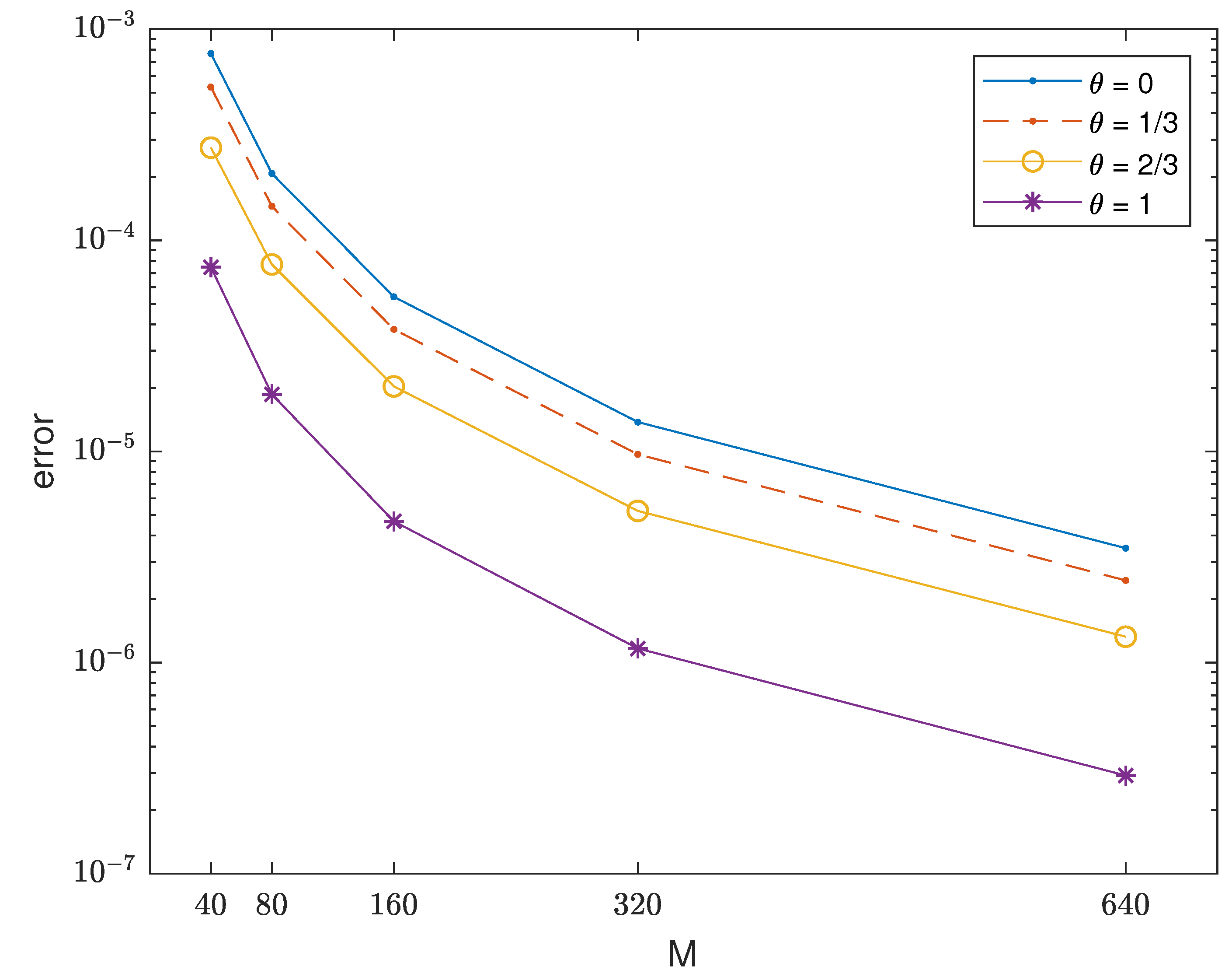
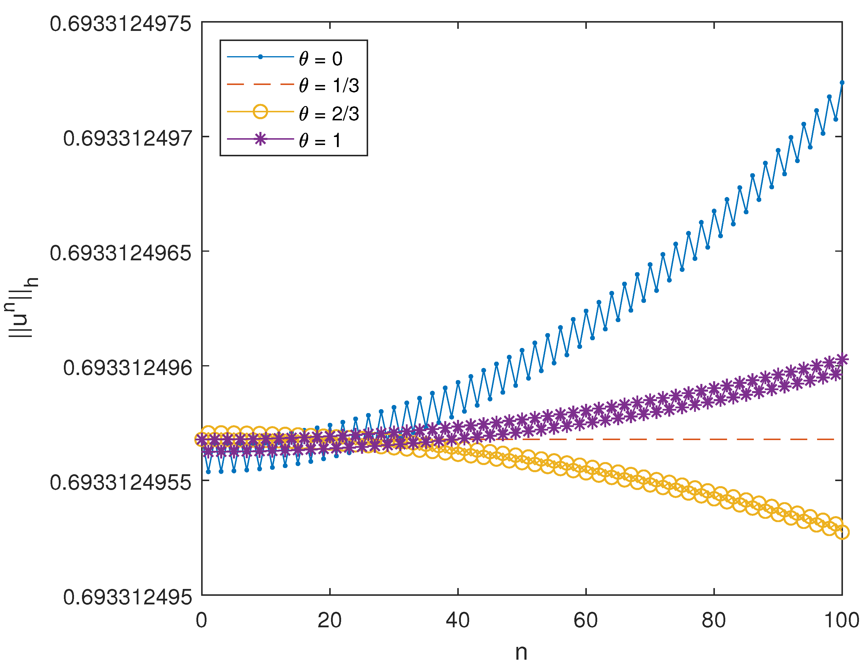
Using domain , final time , and , we obtained an optimal order of convergence as shown in Table 1 and Table 2. The performances for each value of are shown in Figure 1 and Figure 2. We see from Figure 1 that all the errors are vanishing for any value of . However, as shown in Figure 2, the quantity is stable only when .
5.2. Accuracy Test for the Viscous Problem
For the case , we used the non-homogeneous example with provided in [4]. The simulation was conducted on the domain with the final time and . The errors and orders of accuracy are given in Table 3 and Table 4. Note that the optimal order of convergence can be achieved for the viscous problem as well. In Figure 3, all errors are vanishing for any value of .
From the results in Section 5.1 and Section 5.2, we see that the scheme converges uniformly for any value of . However, we see in Figure 2 that the quantity is preserved only when . This agrees with the result from Theorem 4. In the subsequent experiment, we show that the scheme also performs better in a long-time simulation when .
5.3. Invariant-Preserving Test
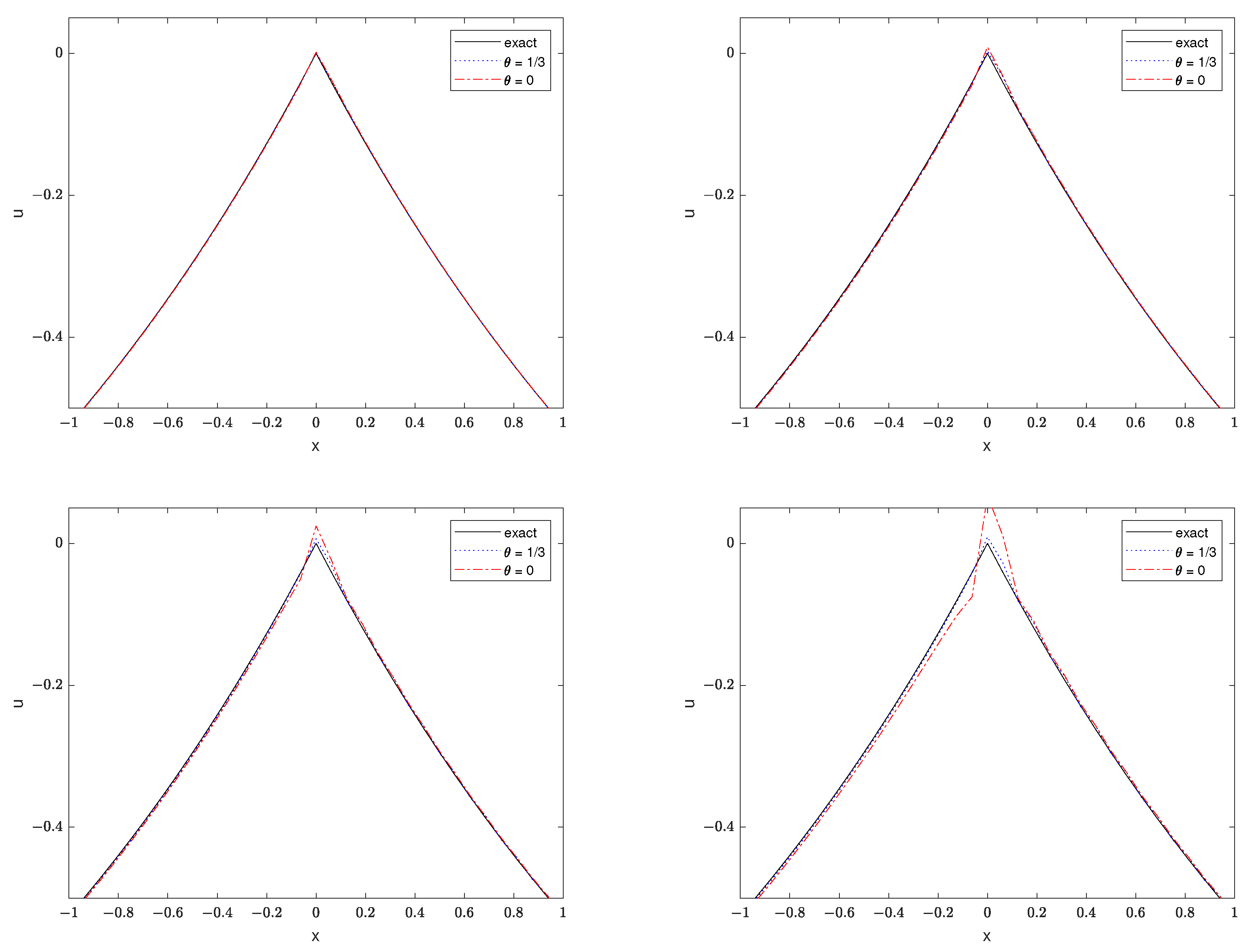
To see how well the scheme performs on a long-time simulation, we tested it on the exact solution with cusp:
and observed how the sharp profile changed over time. The simulation was done using on the domain with time step . In Figure 4, we see that when the scheme preserves the shape of numerical solution, but when we used , the numerical solution becomes unstable as time increases. This shows that the invariant-preserving method performs better in the long run.
5.4. Asymptotic Test
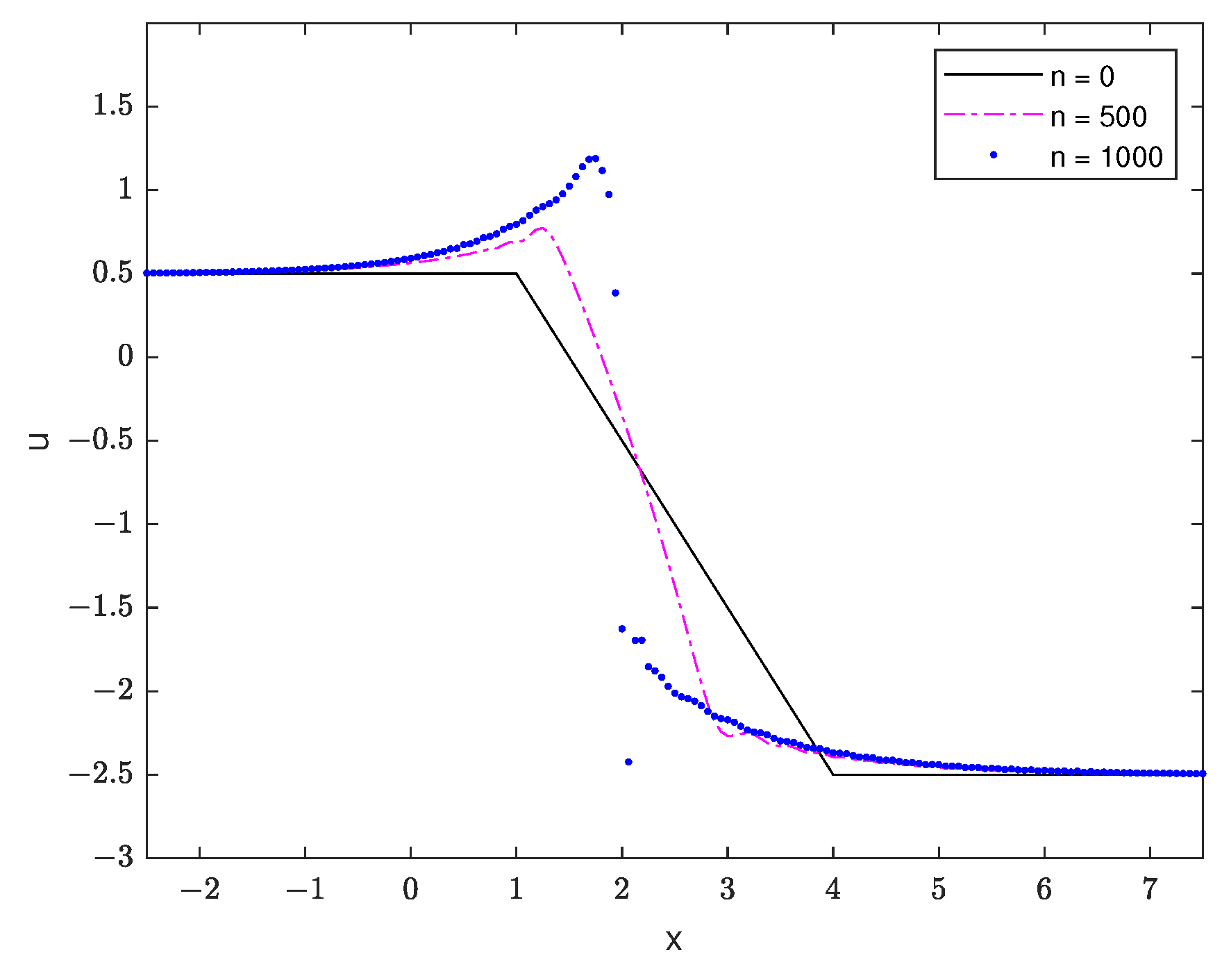
We tested the invariant-preserving scheme () on the initial data
6. Discussion
Results from Section 5 verified that the numerical solutions converge to the exact solutions with second order of accuracy with respect to the spatial variable. The convergence can be inferred from the error plots in Figure 1 and Figure 3 while the rate of convergence can be inferred from the numeric evidence in Table 1, Table 2, Table 3 and Table 4. Note that the second-order convergence occurs at any value of . However, Figure 2 shows that the invariant is preserved only when . This behavior agrees with the results we proved in Section 3. The comparison in Section 5.3 confirmed that the invariant-preserving scheme performs better in the long run. This hints that the invariant-preserving property, if any, should be taken into account when one wants to design a numerical method.
The experiment on the asymptotic problem in Section 5.4 ensured that the proposed scheme is robust and can be applied to a broader range of problems. Possible applications include but are not limited to adaption to other types of boundary conditions, changing to various types of initial data, and adding some extra terms to the equation. All of these possibilities allow us to simulate wider ranges of natural phenomena. On the other hand, one can improve the accuracy of presented. In [19], a fourth-order operator is applied to a viscous Burgers’ equation. The same operator can be applied to the Burgers-Poisson system to obtain a fourth-order method as well. Besides this, the idea of the proposed method can also be generalized to higher dimension. While the simplicity of the finite diffidence method makes the generalization of the implementation straightforward, the analysis part may not be so. One may opt for other approach such as the spectral volume (SV) method [20,21,22] which has high order of accuracy and can be readily applied to higher dimensional settings.
7. Conclusions
In this paper, we proposed a family of implicit finite difference -schemes to solve the system of Burgers-Poisson equations. The method used information from three time levels and eliminated the need to solve unknowns using iterative nonlinear solvers. When , we showed that the resulting scheme has a discrete invariant-preserving property. We also proved that the numerical solution converges uniformly and has second order of accuracy with respect to the spatial variable. Finally, the numerical experiments verified that the optimal order of convergence is achieved for any value of , but the invariant is stable only when . All the numerical evidences obtained from the simulations agree with the theoretical results.
Author Contributions
C.D., M.K. and N.P. contributed equally to this work. All authors have read and agreed to the published version of the manuscript.
Funding
This research was funded by Chiang Mai University. Nattapol Ploymaklam was supported by the Research Fund for DPST Graduate with First Placement [Grant No.036/2015].
Acknowledgments
We wish to thank anonymous referees for their careful readings of the manuscript and helpful suggestions which significantly improve the paper’s quality. We also would like to thank Amiya K. Pani (IIT Bombay, India) for his valuable comments and suggestions. Nattapol Ploymaklam is supported by Chiang Mai University and by the Research Fund for DPST Graduate with First Placement [Grant No.036/2015], The Institute for the Promotion of Teaching Science and Technology (IPST), Thailand, under the mentoring of Piyapong Niamsup.
Conflicts of Interest
The authors declare no conflict of interest.
References
- Korteweg, D.J.; de Vries, G. On the change of form of long waves advancing in a rectangular canal, and on a new type of long stationary waves. Philos. Mag. 1895, 39, 422–443. [Google Scholar] [CrossRef]
- Whitham, G.B. Pure and Applied Mathematics. In Linear and Nonlinear Waves; Wiley-Interscience [John Wiley & Sons]: New York, NY, USA; London, UK; Sydney, Australia, 1974. [Google Scholar]
- Fellner, K.; Schmeiser, C. Burgers-Poisson: A nonlinear dispersive model equation. SIAM J. Appl. Math. 2004, 64, 1509–1525. [Google Scholar] [CrossRef] [Green Version]
- Ploymaklam, N.; Kumbhar, P.M.; Pani, A.K. A Priori Error Anal. Local Discontinuous Galerkin Method Viscous Burgers-Poisson Syst. Int. J. Numer. Anal. Model. 2017, 14, 784–807. [Google Scholar]
- Turgay, N.C.; Hizel, E. Group invariant solutions of Burgers-Poisson equation. Int. Math. Forum 2007, 2, 2701–2710. [Google Scholar] [CrossRef] [Green Version]
- Grunert, K.; Nguyen, K.T. On the Burgers-Poisson equation. J. Differ. Equ. 2016, 261, 3220–3246. [Google Scholar] [CrossRef] [Green Version]
- Camassa, R.; Holm, D.D. An integrable shallow water equation with peaked solitons. Phys. Rev. Lett. 1993, 71, 1661–1664. [Google Scholar] [CrossRef] [Green Version]
- Camassa, R.; Holm, D.D.; Hyman, J.M. A new integrable shallow water equation. In Advances in Applied Mechanics; Elsevier: Amsterdam, The Netherlands, 1994; Volume 31, pp. 1–33. [Google Scholar]
- Benjamin, T.B. Internal waves of permanent form in fluids of great depth. J. Fluid Mech. 1967, 29, 559–592. [Google Scholar] [CrossRef]
- Ono, H. Algebraic solitary waves in stratified fluids. J. Phys. Soc. Jpn. 1975, 39, 1082–1091. [Google Scholar] [CrossRef]
- Rosenau, P. A quasi-continuous description of a nonlinear transmission line. Phys. Scr. 1986, 34, 827–829. [Google Scholar] [CrossRef]
- Rosenau, P. Dynamics of Dense Discrete Systems: High Order Effects. Prog. Theor. Phys. 1988, 79, 1028–1042. [Google Scholar] [CrossRef] [Green Version]
- Peregrine, D.H. Calculations of the development of an undular bore. J. Fluid Mech. 1966, 25, 321–330. [Google Scholar] [CrossRef]
- Peregrine, D.H. Long waves on a beach. J. Fluid Mech. 1967, 27, 815–827. [Google Scholar] [CrossRef]
- Hizel, E.; Küçükarslan, S. A numerical analysis of the Burgers-Poisson (BP) equation using variational iteration method. In Proceedings of the 3rd WSEAS International Conference on Applied and Theoretical Mechanics, Tenerife, Canary Islands, Spain, 14–16 December 2007. [Google Scholar]
- Zeng, C.; Yang, Q.; Zhang, B. Homotopy perturbation method for fractional-order Burgers-Poisson equation. arXiv 2010, arXiv:1003.1828. [Google Scholar]
- Nwamba, J.I. Exact and explicit approximate solutions to the multi-order fractional Burgers-Poisson and fractional Burgers-Poisson equations. Appl. Comput. Math. 2013, 2, 78–85. [Google Scholar] [CrossRef]
- Liu, H.; Ploymaklam, N. A local discontinuous Galerkin method for the Burgers-Poisson equation. Numer. Math. 2015, 129, 321–351. [Google Scholar] [CrossRef] [Green Version]
- Wang, X.; Zhang, Q.; Sun, Z.Z. The pointwise error estimates of two energy-preserving fourth-order compact schemes for viscous Burgers’ equation. Adv. Comput. Math. 2021, 47, 42. [Google Scholar] [CrossRef]
- Kannan, R.; Wang, Z.J. A high order spectral volume solution to the Burgers’ equation using the Hopf-Cole transformation. Int. J. Numer. Methods Fluids 2012, 69, 781–801. [Google Scholar] [CrossRef]
- Kannan, R.; Wang, Z.J. A study of viscous flux formulations for a p-multigrid spectral volume Navier Stokes solver. J. Sci. Comput. 2009, 41, 165–199. [Google Scholar] [CrossRef]
- Kannan, R.; Wang, Z.J. LDG2: A variant of the LDG flux formulation for the spectral volume method. J. Sci. Comput. 2011, 46, 314–328. [Google Scholar] [CrossRef]
- Kannan, R. A high order spectral volume formulation for solving equations containing higher spatial derivative terms: Formulation and analysis for third derivative spatial terms using the LDG discretization procedure. Commun. Comput. Phys. 2011, 10, 1257–1279. [Google Scholar] [CrossRef]
- Kannan, R. A high order spectral volume formulation for solving equations containing higher spatial derivative terms II: Improving the third derivative spatial discretization using the LDG2 method. Commun. Comput. Phys. 2012, 12, 767–788. [Google Scholar] [CrossRef]
- Kuo, P.Y.; Sanz-Serna, J.M. Convergence of methods for the numerical solution of the Korteweg-de Vries equation. IMA J. Numer. Anal. 1981, 1, 215–221. [Google Scholar] [CrossRef]
- Zhang, L. A finite difference scheme for generalized regularized long-wave equation. Appl. Math. Comput. 2005, 168, 962–972. [Google Scholar] [CrossRef]
- Zuo, J.M.; Zhang, Y.M.; Zhang, T.D.; Chang, F. A new conservative difference scheme for the general Rosenau-RLW equation. Bound. Value Probl. 2010, 2010, 516260. [Google Scholar] [CrossRef] [Green Version]
- Pan, X.; Zhang, L. On the convergence of a conservative numerical scheme for the usual Rosenau-RLW equation. Appl. Math. Model. 2012, 36, 3371–3378. [Google Scholar] [CrossRef]
- Wang, X.; Sun, Z.Z. A second order convergent difference scheme for the initial-boundary value problem of Korteweg–de Vires equation. Numer. Methods Partial Differ. Equ. 2021, 37, 2873–2894. [Google Scholar] [CrossRef]
- Zhang, Q.; Qin, Y.; Wang, X.; Sun, Z.Z. The study of exact and numerical solutions of the generalized viscous Burgers’ equation. Appl. Math. Lett. 2021, 112, 106719. [Google Scholar] [CrossRef]
- Hu, J.; Xu, Y.; Hu, B. Conservative Linear Difference Scheme for Rosenau-KdV Equation. Available online: https://www.hindawi.com/journals/amp/2013/423718/ (accessed on 27 September 2021).
- Janwised, J.; Wongsaijai, B.; Mouktonglang, T.; Poochinapan, K. A Modified Three-Level Average Linear-Implicit Finite Difference Method for the Rosenau-Burgers Equation. Available online: https://www.hindawi.com/journals/amp/2014/734067/ (accessed on 27 September 2021).
- Hu, J.; Xu, Y.; Hu, B.; Xie, X. Two conservative difference schemes for Rosenau-Kawahara equation. Adv. Math. Phys. 2014, 11, 217393. [Google Scholar] [CrossRef] [Green Version]
- Wongsaijai, B.; Poochinapan, K. A three-level average implicit finite difference scheme to solve equation obtained by coupling the Rosenau-KdV equation and the Rosenau-RLW equation. Appl. Math. Comput. 2014, 245, 289–304. [Google Scholar] [CrossRef]
- Zhang, Q.; Wang, X.; Sun, Z.Z. The pointwise estimates of a conservative difference scheme for Burgers’ equation. Numer. Methods Partial Differ. Equ. 2020, 36, 1611–1628. [Google Scholar] [CrossRef]
- Zhou, Y. Applications of Discrete Functional Analysis to the Finite Difference Method; Pergamon Press: Oxford, UK, 1991. [Google Scholar]
Figure 1.
Comparison of the uniform errors at when using different values of for the inviscous problem.
Figure 1.
Comparison of the uniform errors at when using different values of for the inviscous problem.

Figure 2.
Values of at when using the scheme with different choices of with on the inviscous problem.
Figure 2.
Values of at when using the scheme with different choices of with on the inviscous problem.

Figure 3.
Comparison of the uniform errors at when using different values of for the viscous problem.
Figure 3.
Comparison of the uniform errors at when using different values of for the viscous problem.

Figure 4.
Comparison between the invariant-preserving scheme () and its counterpart (). Upper left: . Upper right: . Lower left: . Lower right: .
Figure 4.
Comparison between the invariant-preserving scheme () and its counterpart (). Upper left: . Upper right: . Lower left: . Lower right: .

Figure 5.
Asymptotic example: initial data and solutions after 500 and 1000 steps.


Table 1.
Errors and orders showing optimal convergence rates for the inviscous problem, with .
| N | ||||||||
|---|---|---|---|---|---|---|---|---|
| Error | Order | Error | Order | Error | Order | Error | Order | |
| 40 | 6.7498 × 10⁻⁴ | 7.8284 × 10⁻⁴ | 4.2413 × 10⁻⁴ | 5.4619 × 10⁻⁴ | ||||
| 80 | 1.7452 × 10⁻⁴ | 1.95 | 2.0982 × 10⁻⁴ | 1.90 | 1.1021 × 10⁻⁴ | 1.94 | 1.4711 × 10⁻⁴ | 1.89 |
| 160 | 4.4369 × 10⁻⁵ | 1.98 | 5.4335 × 10⁻⁵ | 1.95 | 2.8086 × 10⁻⁵ | 1.97 | 3.8179 × 10⁻⁵ | 1.95 |
| 320 | 1.1186 × 10⁻⁵ | 1.99 | 1.3826 × 10⁻⁵ | 1.97 | 7.0886 × 10⁻⁶ | 1.99 | 9.7254 × 10⁻⁶ | 1.97 |
| 640 | 2.8083 × 10⁻⁶ | 1.99 | 3.4874 × 10⁻⁶ | 1.99 | 1.7806 × 10⁻⁶ | 1.99 | 2.4543 × 10⁻⁶ | 1.99 |
Table 2.
Errors and orders showing optimal convergence rates for the inviscous problem, with .
| N | ||||||||
|---|---|---|---|---|---|---|---|---|
| Error | Order | Error | Order | Error | Order | Error | Order | |
| 40 | 1.7901 × 10⁻⁴ | 2.7492 × 10⁻⁴ | 9.8426 × 10⁻⁵ | 7.4600 × 10⁻⁵ | ||||
| 80 | 4.7136 × 10⁻⁵ | 1.93 | 7.6875 × 10⁻⁵ | 1.84 | 2.4617 × 10⁻⁵ | 2.00 | 1.8652 × 10⁻⁵ | 2.00 |
| 160 | 1.2084 × 10⁻⁵ | 1.96 | 2.0333 × 10⁻⁵ | 1.92 | 6.1550 × 10⁻⁶ | 2.00 | 4.6661 × 10⁻⁶ | 2.00 |
| 320 | 3.0585 × 10⁻⁶ | 1.98 | 5.2290 × 10⁻⁶ | 1.96 | 1.5388 × 10⁻⁶ | 2.00 | 1.1665 × 10⁻⁶ | 2.00 |
| 640 | 7.6934 × 10⁻⁷ | 1.99 | 1.3259 × 10⁻⁶ | 1.98 | 3.8470 × 10⁻⁷ | 2.00 | 2.9163 × 10⁻⁷ | 2.00 |
Table 3.
Errors and orders showing optimal convergence rates for the viscous problem, with .
| N | ||||||||
|---|---|---|---|---|---|---|---|---|
| Error | Order | Error | Order | Error | Order | Error | Order | |
| 80 | 9.8070 × 10⁻¹ | 8.8961 × 10⁻¹ | 1.0900 | 1.0686 | ||||
| 160 | 1.5003 × 10⁻¹ | 2.71 | 1.6312 × 10⁻¹ | 2.45 | 1.4306 × 10⁻¹ | 2.93 | 1.5557 × 10⁻¹ | 2.78 |
| 320 | 3.0028 × 10⁻² | 2.32 | 3.0737 × 10⁻² | 2.41 | 2.9229 × 10⁻² | 2.29 | 3.1383 × 10⁻² | 2.31 |
| 640 | 7.0535 × 10⁻³ | 2.09 | 7.3580 × 10⁻³ | 2.06 | 7.0430 × 10⁻³ | 2.05 | 7.6141 × 10⁻³ | 2.04 |
| 1280 | 1.7182 × 10⁻³ | 2.04 | 1.8173 × 10⁻³ | 2.02 | 1.7445 × 10⁻³ | 2.01 | 1.8972 × 10⁻³ | 2.00 |
Table 4.
Errors and orders showing optimal convergence rates for the viscous problem, with .
| N | ||||||||
|---|---|---|---|---|---|---|---|---|
| Error | Order | Error | Order | Error | Order | Error | Order | |
| 80 | 1.1878 | 1.2909 | 1.2501 | 1.4776 | ||||
| 160 | 1.5447 × 10⁻¹ | 2.94 | 1.7385 × 10⁻¹ | 2.89 | 1.7512 × 10⁻¹ | 2.84 | 2.0320 × 10⁻¹ | 2.86 |
| 320 | 3.3077 × 10⁻² | 2.22 | 3.5948 × 10⁻² | 2.27 | 3.7731 × 10⁻² | 2.21 | 4.1052 × 10⁻² | 2.31 |
| 640 | 8.0712 × 10⁻³ | 2.03 | 8.7244 × 10⁻³ | 2.04 | 9.2118 × 10⁻³ | 2.03 | 9.9053 × 10⁻³ | 2.05 |
| 1280 | 2.0101 × 10⁻³ | 2.01 | 2.1747 × 10⁻³ | 2.00 | 2.2928 × 10⁻³ | 2.01 | 2.4630 × 10⁻³ | 2.01 |
Publisher’s Note: MDPI stays neutral with regard to jurisdictional claims in published maps and institutional affiliations. |
© 2021 by the authors. Licensee MDPI, Basel, Switzerland. This article is an open access article distributed under the terms and conditions of the Creative Commons Attribution (CC BY) license (https://creativecommons.org/licenses/by/4.0/).
Share and Cite
MDPI and ACS Style
Darayon, C.; Khebchareon, M.; Ploymaklam, N. An Invariant-Preserving Scheme for the Viscous Burgers-Poisson System. Computation 2021, 9, 115. https://0-doi-org.brum.beds.ac.uk/10.3390/computation9110115
AMA Style
Darayon C, Khebchareon M, Ploymaklam N. An Invariant-Preserving Scheme for the Viscous Burgers-Poisson System. Computation. 2021; 9(11):115. https://0-doi-org.brum.beds.ac.uk/10.3390/computation9110115
Chicago/Turabian StyleDarayon, Chayapa, Morrakot Khebchareon, and Nattapol Ploymaklam. 2021. "An Invariant-Preserving Scheme for the Viscous Burgers-Poisson System" Computation 9, no. 11: 115. https://0-doi-org.brum.beds.ac.uk/10.3390/computation9110115
Note that from the first issue of 2016, this journal uses article numbers instead of page numbers. See further details here.