Direct Sampling for Recovering Sound Soft Scatterers from Point Source Measurements

Abstract

In this paper, we consider the inverse problem of recovering a sound soft scatterer from the measured scattered field. The scattered field is assumed to be induced by a point source on a curve/surface that is known. Here, we propose and analyze new direct sampling methods for this problem. The first method we consider uses a far-field transformation of the near-field data, which allows us to derive explicit bounds in the resolution analysis for the direct sampling method’s imaging functional. Two direct sampling methods are studied, using the far-field transformation. For these imaging functionals, we use the Funk–Hecke identities to study the resolution analysis. We also study a direct sampling method for the case of the given Cauchy data. Numerical examples are given to show the applicability of the new imaging functionals for recovering a sound soft scatterer with full and partial aperture data.

1. Introduction

Here, we develop new direct sampling methods for recovering a sound soft scatterer from the measured scattered field induced by point sources. Direct (also referred to as orthogonality) sampling methods are qualitative reconstruction methods that have gained interest recently by researchers. These types of reconstruction algorithms were first introduced in [1]. Like other qualitative reconstruction methods, the direct sampling method requires little a priori information about the specific physical parameters of the scatterer. This implies that these methods are robust in the fact that they recover multiple types of scatterers using the same algorithm (see, for example, [2,3,4]). Therefore, these methods can be advantageous to use in applications such as non-destructive testing and medical imaging. Similar methods were also studied in diffuse optical tomography [5], electrical impedance tomography [6] and thermodynamics [7]. These methods were studied in detail for far-field data, but little was done for the case of near-field data. In this paper, we develop and analyze some direct sampling method, given near-field measurements. The methods studied here are applicable in the field of near-field acoustic holography; see [8,9,10].

The main idea behind the methodology of qualitative methods is to develop an imaging functional using the measured data that are positive in the region that you wish to recover and are (approximately) zero outside the region. All qualitative methods achieve this in various ways (see, for example, [11,12]). One of the main advantages of direct sampling methods is the fact that the imaging functional is usually given by an inner product (or norm) of the data operator and a specifically chosen function. This implies that these imaging functionals are simple to compute as well as stable, with respect to noise in the scattering data. The main analytical tool for studying these methods comes from the factorization of the data operator, just as in the factorization method (see, for example, [13,14,15]).

The main idea of this paper is to preform a far-field transformation of the near-field operator. This completely transforms the operator to the corresponding far-field operator for the scattering problem. This has the advantage that we can then use the theory already developed in the literature for the far-field operator as well as avoid using the Helmholtz–Kirchhoff identity, which is often used in reverse time migration [16]. Reverse time migration is very similar to the direct sampling method, but in the case of near-field measurements, the Helmholtz–Kirchhoff identity does not provide explicit decay rates for the resolution analysis. For the case of far-field measurements, one uses the Funk–Hecke identity. This gives explicit bounds on the imaging functionals as $\mathrm{dist}(z,D)\to \infty$, where D denotes the unknown scatterer to be recovered and $z\in {\mathbb{R}}^d$ is the sampling point where we evaluate the imaging functional. Using the asymptotic bounds on the Bessel functions given in the Funk–Hecke identity, we can have theoretical limits on the value of the imaging functional outside the scatterer. We also study a new direct sampling method which uses the measured Cauchy data of the scattered field from point sources.

The rest of the paper is organized as follows. In the next section, we rigorously describe the scattering problem under consideration as well as derive a factorization for the corresponding near-field operator. The factorization for the near-field operator is critical in the development of the new direct sampling methods. Next, we derive two new direct sampling methods, where we use a far-field transformation of the near-field operator. This is done in order to avoid using the Helmholtz–Kirchhoff identity, which is often used in reverse time migration. We also study a direct sampling imaging functional that uses the near-field Cauchy data. For proof of concept, we provide numerical examples for the three imaging functionals studied for both full and partial aperture data.

2. Analysis of the Scattering Problem

In this section, we derive a factorization of the near-field operator that will be used to analyze the new direct sampling methods imaging functionals for recovering a sound soft scatterer from the measured scattered field. To this end, we begin by formulating the direct time-harmonic scattering problem under consideration. The scattered field denoted by $u^s(·,y)$ is induced by a point source incident field $u^i(·,y)=\Phi (·,y)$. Here, we let y denote the location of the point source located on the curves/surface $\Gamma$, and $\Phi (x,y)$ is the radiating fundamental solution to Helmholtz equation given by the following:

$$\Phi (x,y)=\left\{\begin{array}{cc}\frac{\mathrm{i}}{4}{H}_0^{\left(1\right)}\left(k\right|x-y\left|\right)\hfill & \hfill \mathrm{in}{\mathbb{R}}^2\\ & \\ \frac{1}{4\pi }\frac{\exp \left(\mathrm{i}k|x-y|\right)}{|x-y|}\hfill & \hfill \mathrm{in}{\mathbb{R}}^3,\end{array}\right.$$

for $x\ne y$, where $H_0^{\left(1\right)}$ is the first kind Hankel function of the order zero. Throughout the paper, we use the boundary integral operators in our analysis, so we will assume that $\Gamma$ is a class ${\mathcal{C}}^2$–smooth closed curves/surface.

Now, let $D\subset {\mathbb{R}}^d$ (for $d=2,3$) be the sound soft scattering obstacle (possibly with multiple components). We assume that the boundary $\partial D$ is a class ${\mathcal{C}}^2$–smooth closed curve/surface, where the exterior ${\mathbb{R}}^d\backslash \overline{D}$ is connected. Therefore, the radiating time-harmonic scattered field $u^s(x,y)\in H_{\mathrm{loc}}^1({\mathbb{R}}^d\backslash \overline{D})$ given by the point source incident field is the unique solution to the following (see, for example, [17]):

$$\begin{array}{ccc}& & {\Delta }_x{u}^s+k^2{u}^s=0\mathrm{in}{\mathbb{R}}^d\backslash \overline{D}\mathrm{and}{u}^s(·,y)=-\Phi (·,y)\mathrm{on}\partial D\hfill \end{array}$$

(1)

$$\begin{array}{ccc}& & {\partial }_r{u}^s-\mathrm{i}k{u}^s=\mathcal{O}\left(\frac{1}{r^{(d+1)/2}}\right)\mathrm{as}r\to \infty \hfill \end{array}$$

(2)

where $r=\left|x\right|$ with k is the positive wave number. Here, we assume that $k^2$ is not a corresponding Dirichlet eigenvalue for the negative Laplacian in D. The Sommerfeld radiation condition given by (2) is satisfied uniformly in all directions. This gives that we can assume that we have the measured scattering data $u^s(x,y)$ for all $x,y\in \Gamma$, provided that $\mathrm{dist}(\Gamma ,D)>0$. Therefore, we now define the so-called near-field operator as follows:

$$N:L^2(\Gamma )⟼L^2(\Gamma )\mathrm{given}\mathrm{by}\left(Ng\right)\left(x\right)={\int }_{\Gamma }{u}^s(x,y)g\left(y\right)\mathrm{d}s\left(y\right).$$

In order to study the inverse problem of reconstructing the sound soft scattering obstacle D given the near-field measurements, we need to derive a suitable factorization for the near-field operator. In [18], a factorization of the near-field operator was studied, but for our purposes, we need to derive a different factorization.

From the direct scattering problem (1)–(2), we make the ansatz such that the scattered field can be represented by the boundary integral operator $S{L}_{\partial D}:H^{-1/2}(\partial D)\mapsto H_{\mathrm{loc}}^1({\mathbb{R}}^d\backslash \overline{D})$ as follows:

$$\begin{array}{c}\hfill u^s(·,y)=\left(S{L}_{\partial D}\right){\phi }_y\mathrm{where}\left(S{L}_{\partial D}\right){\phi }_y={\int }_{\partial D}\Phi (·,\omega ){\phi }_y\left(\omega \right)\mathrm{d}s\left(\omega \right)\end{array}$$

(3)

for some ${\phi }_y\in H^{-1/2}(\partial D)$. See [19] for the mapping properties of the boundary integral operator $S{L}_{\partial D}$. Therefore, we have that ${\phi }_y$ satisfies the following equation:

$$\left(S_{\partial D\to \partial D}\right){\phi }_y=-\Phi (·,y)\mathrm{for}\mathrm{any}\mathrm{fixed}y\in C$$

where $S_{\partial D\to \partial D}:H^{-1/2}(\partial D)\to H^{1/2}(\partial D)$ is given by the following:

$$\left(S_{\partial D\to \partial D}\right){\phi }_y={\int }_{\partial D}\Phi (·,\omega ){\phi }_y\left(\omega \right)\mathrm{d}s\left(\omega \right){|}_{\partial D}.$$

Note that we have used the continuity of the trace for the boundary integral operator $S{L}_{\partial D}$ on the boundary $\partial D$ (see, for example, [19]). Since $k^2$ is not a Dirichlet eigenvalue of the negative Laplacian in D, Lemma 1.14 of [12] gives that $S_{\partial D\to \partial D}$ has a bounded inverse. We define the bounded linear operator as follows:

$$\begin{array}{c}\hfill T:H^{1/2}(\partial D)⟼H^{-1/2}(\partial D)\mathrm{such}\mathrm{that}T=-S_{\partial D\to \partial D}^{-1}.\end{array}$$

(4)

This implies that the scattered field has the following representation:

$$\begin{array}{c}\hfill u^s(·,y)={\int }_{\partial D}\Phi (·,\omega )\left[T\Phi (·,y)\right]\left(\omega \right)\mathrm{d}s\left(\omega \right).\end{array}$$

(5)

Equation (5) gives us an analytical solution to the direct scattering problem, using boundary integral operators. One can view (5) as a stand in for the Lippmann–Schwinger integral representation of the scattered field that one obtains by considering a penetrable scatterer (see, for example, Equation (8.13) of [17]). From this, we derive a factorization of the near-field operator. To this end, we define the bounded linear operator as follows:

$$\begin{array}{c}\hfill S:L^2(\Gamma )⟼L^2(\partial D)\mathrm{given}\mathrm{by}Sg={\int }_{\Gamma }\Phi (·,y)g\left(y\right)\mathrm{d}s\left(y\right){|}_{\partial D}\end{array}$$

(6)

along with its dual operator

$$\begin{array}{c}\hfill S^{\top }:L^2(\partial D)⟼L^2(\Gamma )\mathrm{given}\mathrm{by}{S}^{\top }\phi ={\int }_{\partial D}\Phi (\omega ,·)\phi \left(\omega \right)\mathrm{d}s\left(\omega \right){|}_{\Gamma }\end{array}$$

(7)

with respect to the bilinear $L^2$ dual product ${\langle ·,·\rangle }_{L^2}$ such that the following holds:

$${\langle \phi ,Sg\rangle }_{L^2(\partial D)}={\langle S^{\top }\phi ,g\rangle }_{L^2(\Gamma )}\mathrm{for}\mathrm{all}g\in L^2(\Gamma )\mathrm{and}\phi \in L^2(\partial D).$$

The single layer potential operators S and $S^{\top }$ defined above are commonly used in studying problems in scattering theory. We can now use the operators defined above to factorize the data operator N. By superposition, we have that

$$w\left(x\right)={\int }_{\Gamma }{u}^s(x,y)g\left(y\right)\mathrm{d}s\left(y\right)\forall x\in {\mathbb{R}}^d\backslash \overline{D}$$

is the scattered field corresponding to (1)–(2) when the point source incident field is replaced by $Sg$ for some $g\in L^2(\Gamma )$ given by (6). Now, appealing to the representation of the scattered field (5), we have the following:

$$w\left(x\right)={\int }_{\partial D}\Phi (x,\omega )\left[TSg\right]\left(\omega \right)\mathrm{d}s\left(\omega \right)\forall x\in {\mathbb{R}}^d\backslash \overline{D}.$$

This implies the following:

$$\begin{array}{c}\hfill {Ng=w|}_{\Gamma }=S^{\top }TSg\mathrm{for}\mathrm{all}g\in L^2(\Gamma )\end{array}$$

(8)

by the above definition of the operators in (6) and (7). Note that the Range$\left(S\right)\subset H^{1/2}(\partial D)$ and $S^{\top }:H^{-1/2}(\partial D)⟼H^{1/2}(\Gamma )$ by the mapping properties in [19]. The factorization of the near-field operator (8) as well as the representation Formula (5) for the scattered field is instrumental in studying the resolution analysis for the direct sampling imaging functionals presented in the following sections.

3. Direct Sampling via Far Field Transform

Now that we have the factorization of the near-field data operator given in (8), we wish to develop new direct sampling methods. To this end, we use far-field transformation for the near-field operator N. We mainly focus on the two-dimensional case, as the three-dimensional case can be handled similarly. The main advantage is that when considering the direct sampling method for far-field data (see, for example, [2,4]) we have that the resolution analysis can easily be obtained by the Funk–Hecke integral identities. Then, the resolution can be derived by the asymptotic decay of the Bessel functions. When considering reverse time migration for near-field data (see, for example, [16]) the analysis uses the Helmholtz–Kirchhoff integral identity, which does not have an explicit decaying of the first-order terms. This means that analytically, one must take the sources/receivers far away from the intended target. Recall, the Funk–Hecke integral identities in [4] are given by the following:

$${\int }_{{\mathbb{S}}^{d-1}}{\mathrm{e}}^{-\mathrm{i}k(z-x)·\widehat{y}}\mathrm{d}s\left(\widehat{y}\right)=\left\{\begin{array}{cc}2\pi J_0\left(k\right|x-z\left|\right)\hfill & \hfill \mathrm{if}d=2,\\ \hfill & \\ 4\pi j_0\left(k\right|x-z\left|\right)\hfill & \hfill \mathrm{if}d=3\end{array}\right.$$

(9)

and when $x\ne z$

$${\int }_{{\mathbb{S}}^{d-1}}\widehat{y}{\mathrm{e}}^{-\mathrm{i}k(z-x)·\widehat{y}}\mathrm{d}s\left(\widehat{y}\right)=\left\{\begin{array}{cc}2\pi \frac{(x-z)}{\mathrm{i}|x-z|}{J}_1\left(k\right|x-z\left|\right)\hfill & \hfill \mathrm{if}d=2,\\ \hfill & \\ 4\pi \frac{(x-z)}{\mathrm{i}|x-z|}{j}_1\left(k\right|x-z\left|\right)\hfill & \hfill \mathrm{if}d=3\end{array}\right.$$

(10)

where ${\mathbb{S}}^{d-1}$ is the unit circle for $d=2$ or unit sphere for $d=3$, i.e., ${\mathbb{S}}^{d-1}=\{p\in {\mathbb{R}}^d:\left|p\right|=1\}$. We make use of the decay of the Bessel functions, i.e., as follows:

$$J_0\left(t\right)=\frac{cost+sint}{\sqrt{\pi t}}\left\{1+\mathcal{O}\left(\frac{1}{t}\right)\right\}\mathrm{and}{J}_1\left(t\right)=\frac{cost-sint}{\sqrt{\pi t}}\left\{-1+\mathcal{O}\left(\frac{1}{t}\right)\right\}$$

for $d=2$ as well as the following:

$$j_0\left(t\right)=\frac{sint}{t}\left\{1+\mathcal{O}\left(\frac{1}{t}\right)\right\}\mathrm{and}{j}_1\left(t\right)=\frac{cost}{t}\left\{-1+\mathcal{O}\left(\frac{1}{t}\right)\right\}$$

for $d=3$ as $t\to \infty$ (see for e.g., [4]).

In order to proceed, we need to define the Dirichlet-to-far-field transformation just as in [3]. This mapping takes the Dirichlet data of the radiating exterior Helmholtz equation in the exterior of $\mathrm{Int}(\Gamma )$ to the corresponding far-field pattern. Here, we let $\mathrm{Int}(\Gamma )$ denote the region enclosed by the collection curve $\Gamma$. Therefore, we have that the Dirichlet-to-far-field transformation $\mathcal{Q}:H^{1/2}(\Gamma )⟼L^2\left({\mathbb{S}}^{d-1}\right)$ is given by the following:

$$\begin{array}{c}\hfill \left(\mathcal{Q}f\right)\left(\widehat{x}\right)=v^{\infty }\left(\widehat{x}\right),\forall \widehat{x}\in {\mathbb{S}}^{d-1}\end{array}$$

(11)

where $v\in H_{\mathrm{loc}}^1({\mathbb{R}}^d\backslash \overline{\mathrm{Int}(\Gamma )})$ is the unique solution to

$$\begin{array}{c}\hfill \Delta v+k^{2}v=0\mathrm{in}{\mathbb{R}}^d\backslash \overline{\mathrm{Int}(\Gamma )}{\mathrm{with}v|}_{\Gamma }=f\end{array}$$

(12)

$$\begin{array}{c}\hfill {\partial }_{r}v-\mathrm{i}kv=\mathcal{O}\left(\frac{1}{r^{(d+1)/2}}\right)\mathrm{as}r\to \infty .\end{array}$$

(13)

Now, we define the far-field pattern $v^{\infty }$, where v has the following expansion:

$$v\left(x\right)=\gamma \frac{{\mathrm{e}}^{\mathrm{i}k\left|x\right|}}{{\left|x\right|}^{(d-1)/2}}\left\{v^{\infty }\left(\widehat{x}\right)+\mathcal{O}\left(\frac{1}{\left|x\right|}\right)\right\}\mathrm{as}\left|x\right|\to \infty$$

where $\widehat{x}:=x/\left|x\right|$ (see Chapter 1 of [12]). Here, the constant is as follows:

$$\gamma =\frac{{\mathrm{e}}^{\mathrm{i}\pi /4}}{\sqrt{8\pi k}}\mathrm{in}{\mathbb{R}}^2\mathrm{and}\gamma =\frac{1}{4\pi }\mathrm{in}{\mathbb{R}}^3.$$

This operator was used in [3] to derive a direct sampling method for both isotropic and anisotropic scatterers. In this section, we see that this can be extended to the case of sound soft scatterers. Additionally, the operator $\mathcal{Q}$ can be constructed without a priori knowledge of D. If $\Gamma$ is a ball centered at the origin with radius $R>0$, i.e., $\Gamma =\partial B(0;R)$, then $\mathcal{Q}$ has an explicit formula via the separation of variables given by the following:

$$\left(\mathcal{Q}f\right)\left(\theta \right)=\underset{0}{\overset{2\pi }{\int }}Q(\theta ,\varphi )f\left(\varphi \right)\mathrm{d}\varphi \mathrm{where}Q(\theta ,\varphi )=\frac{(1-\mathrm{i})}{2\pi \sqrt{\pi k}}\sum _{\left|m\right|=0}^{\infty }\frac{{\mathrm{e}}^{\mathrm{i}m(\theta -\varphi -\pi /2)}}{H_m^{\left(1\right)}\left(kR\right)}$$

with $f\left(\varphi \right):=f\left(R(cos\varphi ,sin\varphi )\right)$; see Section 2 of [3] for details. For our numerical experiments, we truncate the series to approximate the operator $\mathcal{Q}$, which converges geometrically in the operator norm (see [3]).

Remark 1.

When $\Gamma \ne \partial B(0;R)$, we can define the Dirichlet-to-far-field transformation $\mathcal{Q}$ by using the boundary integral equations. See Section 2 of [12] for a detailed construction.

We now show that the near-field operator N for a sound soft scatterer can be transformed into the far-field operator (see Chapter 2 [12]), using the operator $\mathcal{Q}$. Once we have shown this, we can employ similar analysis of the direct sampling methods studied in [2]. Recall, that the single layer potential

$$v\left(x\right)={\int }_{\partial D}\Phi (x,\omega )\phi \left(\omega \right)\mathrm{d}s\left(\omega \right)\mathrm{for}\mathrm{any}\phi \in L^2(\partial D)$$

satisfies (12)–(13) with $f=S^{\top }\phi$ as defined in (7). Note that by the mapping properties of the single layer potential (see Chapter 6 of [19]), we have that the range of $S^{\top }$ is a subset of $H^{1/2}(\Gamma )$. Therefore, by the asymptotic expansion of the fundamental solution (see, for example, [17]) we obtain the following relationship:

$$\begin{array}{c}\hfill \left(\mathcal{Q}{S}^{\top }\phi \right)\left(\widehat{x}\right)={\int }_{\partial D}{\mathrm{e}}^{-\mathrm{i}k\widehat{x}·\omega }\phi \left(\omega \right)\mathrm{d}s\left(\omega \right)\mathrm{for}\mathrm{any}\phi \in L^2(\partial D).\end{array}$$

(14)

Now, motivated by (14), we define the trace of the Herglotz wave function on the boundary $\partial D$ as the bounded linear operator $H:L^2\left({\mathbb{S}}^{d-1}\right)⟼L^2(\partial D)$ given by the following:

$$\left(Hg\right)\left(\omega \right)={\int }_{{\mathbb{S}}^{d-1}}{\mathrm{e}}^{\mathrm{i}k\omega ·\widehat{x}}g\left(\widehat{x}\right)\mathrm{d}s\left(\widehat{x}\right){|}_{\partial D}\mathrm{for}\mathrm{any}g\in L^2\left({\mathbb{S}}^{d-1}\right).$$

Now, we recall the adjoint operator $H^{*}:L^2(\partial D)⟼L^2\left({\mathbb{S}}^{d-1}\right)$ such that the following holds:

$${(Hg,\phi )}_{L^2(\partial D)}={(g,H^{*}\phi )}_{L^2\left({\mathbb{S}}^{d-1}\right)}\mathrm{for}\mathrm{all}g\in L^2\left({\mathbb{S}}^{d-1}\right)\mathrm{and}\phi \in L^2(\partial D)$$

which is given by the following:

$$\left(H^{*}\phi \right)\left(\widehat{x}\right)={\int }_{\partial D}{\mathrm{e}}^{-\mathrm{i}k\widehat{x}·\omega }\phi \left(\omega \right)\mathrm{d}s\left(\omega \right)\mathrm{for}\mathrm{any}\phi \in L^2(\partial D)$$

(see, for example, [12] Chapter 2). Therefore, by appealing to (14) we have the following:

$$\mathcal{Q}{S}^{\top }\phi =H^{*}\phi \mathrm{for}\mathrm{any}\phi \in L^2\left(D\right).$$

From this, we have that the dual operator of ${\left(H^{*}\right)}^{\top }:L^2\left({\mathbb{S}}^{d-1}\right)⟼L^2(\partial D)$ satisfies the following:

$$S{\mathcal{Q}}^{\top }={\left(H^{*}\right)}^{\top }\mathrm{with}\mathrm{the}\mathrm{operator}\left({\left(H^{*}\right)}^{\top }g\right)\left(\omega \right):={\int }_{{\mathbb{S}}^{d-1}}{\mathrm{e}}^{-\mathrm{i}k\omega ·\widehat{x}}g\left(\widehat{x}\right)\mathrm{d}s\left(\widehat{x}\right){|}_{\partial D}$$

for all $g\in L^2\left({\mathbb{S}}^{d-1}\right)$ (see, for example, Chapter 2 of [20]). To continue, we notice the following:

$$\begin{array}{cc}\hfill \left({\left(H^{*}\right)}^{\top }g\right)\left(\omega \right)& ={\int }_{{\mathbb{S}}^{d-1}}{\mathrm{e}}^{-\mathrm{i}k\omega ·\widehat{x}}g\left(\widehat{x}\right)\mathrm{d}s\left(\widehat{x}\right){|}_{\partial D}\hfill \\ \hfill & ={\int }_{{\mathbb{S}}^{d-1}}{\mathrm{e}}^{\mathrm{i}k\omega ·\widehat{x}}g(-\widehat{x})\mathrm{d}s\left(\widehat{x}\right){|}_{\partial D}\hfill \\ \hfill & =\left(H\mathcal{R}g\right)\left(\omega \right)\hfill \end{array}$$

where the operator $\mathcal{R}:L^2\left({\mathbb{S}}^{d-1}\right)⟼L^2\left({\mathbb{S}}^{d-1}\right)$ is given by $\left(\mathcal{R}g\right)\left(\widehat{x}\right)=g(-\widehat{x})$. It is clear that $\mathcal{R}$ is a bounded linear operator and $\mathcal{R}={\mathcal{R}}^{-1}$. By the definition of the operators $\mathcal{Q}$ and $\mathcal{R}$, we can conclude the following:

$$\begin{array}{c}\hfill \mathcal{Q}N{\mathcal{Q}}^{\top }\mathcal{R}=H^{*}TH\mathrm{where}\mathcal{Q}N{\mathcal{Q}}^{\top }\mathcal{R}:L^2\left({\mathbb{S}}^{d-1}\right)⟼L^2\left({\mathbb{S}}^{d-1}\right)\end{array}$$

(15)

by appealing to the factorization in (8). Note, by Equation (1.55) in [12], we can conclude that $\mathcal{Q}N{\mathcal{Q}}^{\top }\mathcal{R}$ corresponds to the far-field operator for the scattering problem (1)–(2), where the incident field is a plane wave.

The imaging functional via far-field transform: We now have all we need to define two new imaging functionals via the transformed operator $\mathcal{Q}N{\mathcal{Q}}^{\top }\mathcal{R}$. For each sampling point $z\in {\mathbb{R}}^d$, the imaging functional via the far-field transform is given by the following:

$$\begin{array}{c}\hfill W_{\mathrm{FF}}\left(z\right)=\left|{\left(\mathcal{Q}N{\mathcal{Q}}^{\top }\mathcal{R}{\varphi }_z,{\varphi }_z\right)}_{L^2\left({\mathbb{S}}^{d-1}\right)}\right|\mathrm{where}{\varphi }_z\left(\widehat{x}\right)={\mathrm{e}}^{-\mathrm{i}kz·\widehat{x}}.\end{array}$$

(16)

Due to the fact that $\mathcal{Q}N{\mathcal{Q}}^{\top }\mathcal{R}$ transforms the near-field operator N for (1)–(2) into the corresponding far-field operator, we can appeal to the results in [2].

Theorem 1.

Let the imaging functional $W_{\mathrm{FF}}\left(z\right)$ be as defined by (16). Then, for any sampling point $z\in {\mathbb{R}}^d\backslash \overline{D}$, we have the following:

$$W_{\mathrm{FF}}\left(z\right)=\mathcal{O}\left(\mathrm{dist}{(z,D)}^{1-d}\right)\mathrm{as}\mathrm{dist}(z,D)\to \infty .$$

Proof. 

In order to prove the result, we let $v_g$ denote the Herglotz wave function for any $x\in {\mathbb{R}}^d$ given by the following:

$$v_g\left(x\right)={\int }_{{\mathbb{S}}^{d-1}}{\mathrm{e}}^{\mathrm{i}kx·\widehat{y}}g\left(\widehat{y}\right)\mathrm{d}s\left(\widehat{y}\right).$$

Here, we can see that $v_g\in H_{\mathrm{loc}}^1\left({\mathbb{R}}^d\right)$ for any given $g\in L^2\left({\mathbb{S}}^{d-1}\right)$, which then implies that $v_g{|}_{\partial D}=Hg\in H^{1/2}(\partial D)$. Therefore, just as in [2], we see that for any $z\in {\mathbb{R}}^d$, we have the following:

$$\begin{array}{cc}\hfill \left|{\left(\mathcal{Q}N{\mathcal{Q}}^{\top }\mathcal{R}{\varphi }_z,{\varphi }_z\right)}_{L^2\left({\mathbb{S}}^{d-1}\right)}\right|& =\left|{(TH{\varphi }_z,H{\varphi }_z)}_{L^2(\partial D)}\right|\mathrm{by}\mathrm{Equation}(15)\hfill \\ \hfill & \le C\parallel H{\varphi }_z{\parallel }_{H^{1/2}(\partial D)}^2\mathrm{by}\mathrm{the}\mathrm{boundedness}\mathrm{of}T\hfill \\ \hfill & =C\parallel v_{{\varphi }_z}{\parallel }_{H^{1/2}(\partial D)}^2\mathrm{by}\mathrm{the}\mathrm{definition}\mathrm{of}{v}_g\hfill \\ \hfill & \le C\parallel v_{{\varphi }_z}{\parallel }_{H^1\left(D\right)}^2\mathrm{by}\mathrm{the}\mathrm{Trace}\mathrm{Theorem}.\hfill \end{array}$$

See, for example, [21] for the Trace Theorem. Now, by the definition of the Herglotz wave function and the Funk–Hecke integral identities (9)–(10), we have the following:

$$\parallel v_{{\varphi }_z}{\parallel }_{H^1\left(D\right)}^2=\mathcal{O}\left(\mathrm{dist}{(z,D)}^{1-d}\right)\mathrm{as}\mathrm{dist}(z,D)\to \infty$$

where we used the decay of the Bessel functions.    □

The result in Theorem 1 is the same as in Theorem 1 in [2]. This is due to the fact that we have transformed the near-field operator into the far-field operator. A similar construction was considered in Section 2.4 of [12], where boundary integral operators were used. Here, we avoid the complex computational set up by not appealing to boundary integral operators to define the imaging functional when $\Gamma$ is a circle/sphere. By Theorem 2.8 of [4], we have that the imaging functional $W_{\mathrm{FF}}\left(z\right)$ is stable with respect to perturbations in the operator N.

By further appealing to the results in [2], we can construct another direct sampling imaging functional, using the transformed operator $\mathcal{Q}N{\mathcal{Q}}^{\top }\mathcal{R}$. We note that the analysis in Chapter 1 of [12] gives that the compact operator $\mathcal{Q}N{\mathcal{Q}}^{\top }\mathcal{R}$ is injective and has a complete orthonormal eigensystem in $L^2\left({\mathbb{S}}^{d-1}\right)$, provided that $k^2$ is not a Dirichlet eigenvalue of the negative Laplacian in D. Let $({\lambda }_j,{\psi }_j)\in \mathbb{C}\backslash \left\{0\right\}\times L^2\left({\mathbb{S}}^{d-1}\right)$ be the orthonormal eigensystem for the operator $\mathcal{Q}N{\mathcal{Q}}^{\top }\mathcal{R}$. Therefore, we can define the following:

$$|\mathcal{Q}N{\mathcal{Q}}^{\top }{\mathcal{R}|}^{p}g=\sum _{j=1}^{\infty }{|{\lambda }_j|}^p{(g,{\psi }_j)}_{{}_{L^2\left({\mathbb{S}}^{d-1}\right)}}{\psi }_j$$

for any fixed $p>0$, where the set $\left\{{\psi }_j\right\}$ is an orthonormal basis in $L^2\left({\mathbb{S}}^{d-1}\right)$. Then, we have that the factorization method can be used to recover the scatterer D (see for e.g., [15]) which gives the result that the following is solvable:

$$\begin{array}{c}\hfill |\mathcal{Q}N{\mathcal{Q}}^{\top }\mathcal{R}{|}^{1/2}{g}_z={\varphi }_z\mathrm{for}z\in {\mathbb{R}}^d\end{array}$$

(17)

if and only if the sampling point $z\in D$. In [2], a connection between the Tikhonov regularized solution to (17) was used to develop another imaging functional. To derive the new imaging functional, we define the Tikhonov filter function for (17) given by the following:

$${\Gamma }_{\alpha }\left(t\right)=\frac{\sqrt{t}}{\alpha +t}\mathrm{on}\mathrm{the}\mathrm{interval}\left[0,\parallel \mathcal{Q}N{\mathcal{Q}}^{\top }\mathcal{R}\parallel \right]$$

which is a continuous function on the given interval. Here, we let $\alpha >0$ denote the fixed regularization parameter. See [22] for the study of regularization techniques and the factorization method. From this, we have that for every $\epsilon >0$, there is an approximating polynomial $P_{\alpha ,\epsilon }\left(t\right)$ such that the following holds:

$$\begin{array}{c}\hfill \parallel P_{\alpha ,\epsilon }\left(t\right)-{\Gamma }_{\alpha }{\left(t\right)\parallel }_{L^{\infty }}<\epsilon \mathrm{on}\mathrm{the}\mathrm{interval}\left[0,\parallel \mathcal{Q}N{\mathcal{Q}}^{\top }\mathcal{R}\parallel \right].\end{array}$$

(18)

Using the polynomial approximate $P_{\alpha ,\epsilon }\left(t\right)$ for the filter function, we can define a new imaging functional.

The imaging functional via Tikhonov regularization: This imaging functional derived from the Tikhonov regularization of (17) for fixed regularization parameter $\alpha >0$ and approximation error ε is given by the following:

$$\begin{array}{c}\hfill W_{\mathrm{TDSM}}\left(z\right)={∥P_{\alpha ,\epsilon }\left(\left|\mathcal{Q}N{\mathcal{Q}}^{\top }\mathcal{R}\right|\right){\varphi }_z∥}_{L^2\left({\mathbb{S}}^{d-1}\right)}^2\mathrm{with}{\varphi }_z\left(\widehat{x}\right)={\mathrm{e}}^{-\mathrm{i}kz·\widehat{x}}.\end{array}$$

(19)

where the polynomial $P_{\alpha ,\epsilon }$ satisfies $P_{\alpha ,\epsilon }\left(t\right)={\Gamma }_{\alpha }\left(t\right)+\mathcal{O}(\epsilon )$ as $\epsilon \to 0$. From this, we have the following result by the analysis in [2]. The imaging functional given in (19) was motivated by the work in [23], and we extend that work to the case of near-field data. There are some interesting questions when considering the implementation of the $W_{\mathrm{TDSM}}\left(z\right)$ such as the following: how to pick $\alpha$ and which polynomial approximation method works best for constructing $P_{\alpha ,\epsilon }\left(t\right)$. Even with these unanswered questions, our numerical experiments show that $W_{\mathrm{TDSM}}\left(z\right)$ can provide good restrictions of the scatterer for a simple least-squares polynomial approximation and without having to find an optimal regularization parameter.

Theorem 2.

Let the imaging functional $W_{\mathrm{TDSM}}\left(z\right)$ be as defined by (19). Then for any sampling point $z\in {\mathbb{R}}^d\backslash \overline{D}$, we have the following: $\exists C_{\alpha }>0$ independent of z such that

$$W_{\mathrm{TDSM}}\left(z\right)\le C_{\alpha }{W}_{\mathrm{FF}}\left(z\right)+\mathcal{O}(\epsilon )\mathrm{as}\epsilon \to 0$$

for all fixed $\alpha >0$ provided that $P_{\alpha ,\epsilon }\left(t\right)={\Gamma }_{\alpha }\left(t\right)+\mathcal{O}(\epsilon )$ as $\epsilon \to 0$.

Proof. 

For the proof of Theorem 2, see Section 4 of [2] to avoid repetition.    □

The imaging functional provided in (19) is equivalent to the one studied in [2] where one has the far-field operator, which corresponds to $\mathcal{Q}N{\mathcal{Q}}^{\top }\mathcal{R}$. We also note that even though the stability of the imaging functional $W_{\mathrm{TDSM}}\left(z\right)$ is not established, our numerical experiments with added noise in the data still provide good reconstructions. Additionally, with the numerical experiments provided in [2], it is seen that $W_{\mathrm{TDSM}}\left(z\right)$ provides better reconstructions than $W_{\mathrm{FF}}\left(z\right)$ in ${\mathbb{R}}^3$. This is not verified theoretically, but the multiple examples in [2] would seem to suggest this to be true.

Notice that just like the Dirichlet-to-far-field transformation $\mathcal{Q}$, we can construct the operator $\mathcal{R}$ without a priori knowledge of D. We also see that $\mathcal{R}$ can easily and efficiently be approximated numerically. To do so, we write the operator as an integral operator with an explicit kernel function. From the fact that $\widehat{x}=(cos\theta ,sin\theta )$ for $\theta \in [0,2\pi )$ if $d=2$, we let $g\left(\theta \right)=g\left((cos\theta ,sin\theta )\right)$. This implies the following:

$$\begin{array}{c}\hfill \left(\mathcal{R}g\right)\left(\theta \right)=g(\theta +\pi )\end{array}$$

(20)

where we used the sum of angles formula to obtain the following equalities:

$$-cos\left(\theta \right)=cos(\theta +\pi )\mathrm{and}-sin\left(\theta \right)=sin(\theta +\pi ).$$

Now, using the Fourier series for $g\left(\theta \right)$, we have the following:

$$g\left(\theta \right)=\sum _{\left|m\right|=0}^{\infty }{g}_m{\mathrm{e}}^{\mathrm{i}m\theta }\mathrm{where}{g}_m=\frac{1}{2\pi }\underset{0}{\overset{2\pi }{\int }}g\left(\varphi \right){\mathrm{e}}^{-\mathrm{i}m\varphi }\mathrm{d}\varphi \mathrm{for}\mathrm{all}m\in \mathbb{Z}.$$

Therefore, by the definition of the operator $\mathcal{R}$ in Equation (20), we obtain the following:

$$\left(\mathcal{R}g\right)\left(\theta \right)=\underset{0}{\overset{2\pi }{\int }}R(\theta ,\varphi )g\left(\varphi \right)\mathrm{d}\varphi \mathrm{where}R(\theta ,\varphi )=\frac{1}{2\pi }\sum _{\left|m\right|=0}^{\infty }{\mathrm{e}}^{\mathrm{i}m(\theta -\varphi +\pi )}$$

by using (20) as well as the Fourier series for g. In order to numerically compute the direct sampling methods imaging functionals, we need a way to compute $\left(\mathcal{R}g\right)\left(\theta \right)$. To this end, we give a result that implies that $\mathcal{R}$ can be approximated by a truncated series for sufficiently smooth g.

Lemma 1.

Let $\mathcal{R}:H^p(0,2\pi )⟼L^2(0,2\pi )$ be the operator defined by (20) and ${\mathcal{R}}_M:H^p(0,2\pi )⟼L^2(0,2\pi )$ be the truncated series for some $M\in \mathbb{N}$ with $p>0$. Then we have norm-convergence with the convergence rate given by the following:

$$\parallel \mathcal{R}-{\mathcal{R}}_M{\parallel }_{H^p(0,2\pi )\mapsto L^2(0,2\pi )}=\mathcal{O}\left(\frac{1}{M^p}\right),\mathrm{as}M⟶\infty .$$

Proof. 

To begin, we clearly see the following:

$$(\mathcal{R}-{\mathcal{R}}_M)g=\frac{1}{2\pi }\sum _{\left|m\right|=M+1}^{\infty }{g}_m{\mathrm{e}}^{\mathrm{i}m(\theta +\pi )}.$$

To prove the claim, we now estimate the $L^2(0,2\pi )$–norm of $(\mathcal{R}-{\mathcal{R}}_M)g$ which is given by the following:

$$\parallel (\mathcal{R}-{\mathcal{R}}_M){g\parallel }_{L^2(0,2\pi )}^2=\sum _{\left|m\right|=M+1}^{\infty }{\left|{\mathrm{e}}^{\mathrm{i}m\pi }{g}_m\right|}^2.$$

where we have used the fact that $|{\mathrm{e}}^{\mathrm{i}m\pi }|=1$ for any $m\in \mathbb{Z}$. Now, we have the following estimate:

$$\begin{array}{cc}\hfill \parallel (\mathcal{R}-{\mathcal{R}}_M){g\parallel }_{L^2(0,2\pi )}^2& =\sum _{\left|m\right|=M+1}^{\infty }\frac{{(1+|m|}^2{)}^p}{{(1+|m|}^2{)}^p}{\left|g_m\right|}^2\hfill \\ \hfill & \le \frac{1}{{(1+M^2)}^p}\sum _{\left|m\right|=M+1}^{\infty }{(1+|m|}^2{)}^p{\left|g_m\right|}^2\hfill \\ \hfill & \le \frac{1}{M^{2p}}{\parallel g\parallel }_{H^p(0,2\pi )}^2.\hfill \end{array}$$

Taking the supremum over g with unit norm in $H^p(0,2\pi )$ proves the claim.    □

Remark 2.

Even though we only focus on the analysis in ${\mathbb{R}}^2$, it is clear that one can define $\mathcal{R}$ similarly in ${\mathbb{R}}^3$. In ${\mathbb{R}}^3$, one can use spherical harmonics to define the operator as well as prove a similar approximation result as in Lemma 1.

Recall that in order to compute the imaging functionals $W_{\mathrm{FF}}\left(z\right)$ and $W_{\mathrm{TDSM}}\left(z\right)$ given by Equations (16) and (19), respectively, we need to evaluate $\mathcal{R}{\varphi }_z$. Since ${\varphi }_z$ is given by a plane wave, we have that it is a smooth function. This implies that ${\mathcal{R}}_M{\varphi }_z\approx \mathcal{R}{\varphi }_z$, where the truncation M can be taken to be reasonably small. In Section 5, we see that $M=10$ gives good reconstructions of the scatterer D when used to truncate the operators $\mathcal{R}$ and $\mathcal{Q}$ for both of the imaging functionals studied in this section.

4. Direct Sampling with Cauchy Data

In this section, we consider another direct sampling method imaging functional provided that one has access to the Cauchy data for the scattering problem (1)–(2). The main idea is to use the representation of the solution given in (5) to establish the resolution analysis. The imaging functional we consider was studied for the case when the scatterer is either isotropic or anisotropic in [3]. The analysis of the imaging functional studied here was not done for the case of a sound soft scatterer, which is the case in this paper. Therefore, in this section, we assume that we have the ‘measured’ Cauchy data.

Remark 3.

Notice that if only the scattered field $u^s(x,y)$ is given for all $x,y\in \Gamma$, then one can compute the normal derivative ${\partial }_{\nu }{u}^s(x,y)$ on Γ. This can be done by computing the scattered field on the exterior of Int$(\Gamma )$ by using a similar formulation as in (3).

The imaging functional for Cauchy data: Assume that we have the Cauchy data $u^s(x,y)$ and ${\partial }_{\nu }{u}^s(x,y)$ for all $x,y\in \Gamma$ that corresponds to the scattering problem (1)–(2). Then, we define the following imaging functional:

$$\begin{array}{c}\hfill W_{\mathrm{CD}}\left(z\right)={\int }_{\Gamma }{\left|{\int }_{\Gamma }{\partial }_{\nu }\overline{\Phi (x,z)}{u}^s(x,y)-\overline{\Phi (x,z)}{\partial }_{\nu }{u}^s(x,y)\mathrm{d}s\left(x\right)\right|}^{\rho }\mathrm{d}s\left(y\right)\end{array}$$

(21)

where $\rho >0$ is a positive constant. Here, again, $\Phi$ corresponds to the radiating fundamental solution to Helmholtz equation. Additionally, the normal derivative, with respect to the x variable, is such that ${\partial }_{\nu }=\nu \left(x\right)·{\nabla }_x$ for any $x\in \Gamma$.

In order to analyze the imaging functional $W_{\mathrm{CD}}\left(z\right)$, we first recall that by (5), we have that the scattered field is given by the following:

$$u^s(x,y)={\int }_{\partial D}\Phi (x,\omega )\left[T\Phi (·,y)\right]\left(\omega \right)\mathrm{d}s\left(\omega \right)\mathrm{for}\mathrm{any}x,y\in \Gamma$$

where $T:H^{1/2}(\partial D)⟼H^{-1/2}(\partial D)$ is a bounded linear operator, provided that $k^2$ is not a Dirichlet eigenvalue of the negative Laplacian in D. We derive an equivalent expression for the imaging functional $W_{\mathrm{CD}}\left(z\right)$ such that the dependence on $\partial D$ is made more explicit. To this end, by taking the normal derivative on $\Gamma$ of the above representation of the scattered field, we have the following:

$${\partial }_{\nu }{u}^s(x,y)={\int }_{\partial D}{\partial }_{\nu }\Phi (x,\omega )\left[T\Phi (·,y)\right]\left(\omega \right)\mathrm{d}s\left(\omega \right)\mathrm{for}\mathrm{any}x,y\in \Gamma .$$

Notice that by using the above representations of the Cauchy data for $u^s(x,y)$ and ${\partial }_{\nu }{u}^s(x,y)$, we have the following:

$$\begin{array}{cc}\hfill & {\int }_{\Gamma }{\partial }_{\nu }\overline{\Phi (x,z)}{u}^s(x,y)-\overline{\Phi (x,z)}{\partial }_{\nu }{u}^s(x,y)\mathrm{d}s\left(x\right)\hfill \\ \hfill & ={\int }_{\Gamma }\left[{\partial }_{\nu }\overline{\Phi (x,z)}{\int }_{\partial D}\Phi (x,\omega )T\Phi (·,y)\mathrm{d}s\left(\omega \right)-\overline{\Phi (x,z)}{\int }_{\partial D}{\partial }_{\nu }\Phi (x,\omega )T\Phi (·,y)\mathrm{d}s\left(\omega \right)\right]\mathrm{d}s\left(x\right)\hfill \\ \hfill & ={\int }_{\Gamma }{\int }_{\partial D}\left[{\partial }_{\nu }\overline{\Phi (x,z)}\Phi (x,\omega )-\overline{\Phi (x,z)}{\partial }_{\nu }\Phi (x,\omega )\right]T\Phi (·,y)\mathrm{d}s\left(\omega \right)\mathrm{d}s\left(x\right)\hfill \\ \hfill & ={\int }_{\partial D}\left[{\int }_{\Gamma }{\partial }_{\nu }\overline{\Phi (x,z)}\Phi (x,\omega )-\overline{\Phi (x,z)}{\partial }_{\nu }\Phi (x,\omega )\mathrm{d}s\left(x\right)\right]T\Phi (·,y)\mathrm{d}s\left(\omega \right).\hfill \end{array}$$

From the analysis in Section 2.2 of [3] we have the following:

$$\frac{1}{2\mathrm{i}}\Im \Phi (z,\omega )={\int }_{\Gamma }\left[{\partial }_{\nu }\overline{\Phi (x,z)}\Phi (x,\omega )-\overline{\Phi (x,z)}{\partial }_{\nu }\Phi (x,\omega )\right]\mathrm{d}s\left(x\right).$$

This is a simple consequence of Green’s second identity and the symmetry of the fundamental solution. Therefore, we have that the imaging functional is equivalent to the following:

$$W_{CD}\left(z\right)={\int }_{\Gamma }{\left|{\int }_{\partial D}\frac{1}{2\mathrm{i}}\Im \Phi (z,\omega )[T\Phi (·,y)]\left(\omega \right)\mathrm{d}s\left(\omega \right)\right|}^{\rho }\mathrm{d}s\left(y\right)$$

where we recall that

$$\Im \Phi (z,\omega )=\left\{\begin{array}{cc}\frac{1}{4}{J}_0\left(k\right|\omega -z\left|\right)\hfill & \hfill \mathrm{if}d=2,\\ & \\ \frac{1}{4\pi }{j}_0\left(k\right|\omega -z\left|\right)\hfill & \hfill \mathrm{if}d=3.\end{array}\right.$$

As we see by the equivalent representation of $W_{CD}\left(z\right)$, we have that the inner integral is in terms of a Bessel function kernel, which will be maximal when z is on $\partial D$ but will decay as the sampling point moves away from the scatterer.

Theorem 3.

Let the imaging functional $W_{\mathrm{CD}}\left(z\right)$ be as defined by (21). Then for any sampling point $z\in {\mathbb{R}}^d\backslash \overline{D}$, we have the following:

$$W_{\mathrm{CD}}\left(z\right)=\mathcal{O}\left(\mathrm{dist}{(z,D)}^{(1-d)\rho /2}\right)\mathrm{as}\mathrm{dist}(z,D)\to \infty \mathrm{for}d=2,3.$$

Proof. 

To begin, we first recall that $T:H^{1/2}(\partial D)⟼H^{-1/2}(\partial D)$ is a bounded linear operator, provided that $k^2$ is not a Dirichlet eigenvalue of the negative Laplacian in D. Therefore, we have the following estimates:

$$\begin{array}{cc}\hfill W_{CD}\left(z\right)& ={\int }_{\Gamma }{\left|{\int }_{\partial D}\frac{1}{2\mathrm{i}}\Im \Phi (z,\omega )[T\Phi (·,y)]\left(\omega \right)\mathrm{d}s\left(\omega \right)\right|}^{\rho }\mathrm{d}s\left(y\right)\hfill \\ \hfill & \le {C\parallel \Im \Phi (z,·)\parallel }_{H^{1/2}(\partial D)}^{\rho }{\int }_{\Gamma }{\parallel T\Phi (·,y)\parallel }_{H^{-1/2}(\partial D)}^{\rho }\mathrm{d}s\left(y\right)\mathrm{by}\mathrm{the}\mathrm{dual}-\mathrm{pairing}\hfill \\ \hfill & \le {C\parallel \Im \Phi (z,·)\parallel }_{H^{1/2}(\partial D)}^{\rho }{\int }_{\Gamma }{\parallel \Phi (·,y)\parallel }_{H^{1/2}(\partial D)}^{\rho }\mathrm{d}s\left(y\right)\mathrm{by}\mathrm{the}\mathrm{boundedness}\mathrm{of}T\hfill \\ \hfill & \le {C\parallel \Im \Phi (z,·)\parallel }_{H^1\left(D\right)}{\int }_{\Gamma }{\parallel \Phi (·,y)\parallel }_{H^1\left(D\right)}^{\rho }\mathrm{d}s\left(y\right)\mathrm{by}\mathrm{the}\mathrm{Trace}\mathrm{Theorem}.\hfill \end{array}$$

Notice that $\Phi (·,y)$ restricted to the scatterer D is a smooth function for every $y\in \Gamma$ since we have assumed that $\mathrm{dist}(\Gamma ,D)>0$. Then, we obtain the following:

$${\int }_{\Gamma }{\parallel \Phi (·,y)\parallel }_{H^1\left(D\right)}^{\rho }\mathrm{d}s\left(y\right)={\parallel \Phi \parallel }_{L^{\rho }\left[\Gamma ;H^1\left(D\right)\right]}^{\rho }$$

which is a fixed constant depending on D and $\Gamma$. Therefore, we have the following:

$$W_{CD}\left(z\right)\le C{\parallel \Im \Phi (z,·)\parallel }_{H^1\left(D\right)}^{\rho }$$

and we then use the fact that

$$\parallel J_0\left(k\right|·-{z\left|\right)\parallel }_{H^1\left(D\right)}=\mathcal{O}\left(\mathrm{dist}{(z,D)}^{-1/2}\right)\mathrm{and}\parallel j_0\left(k\right|·-{z\left|\right)\parallel }_{H^1\left(D\right)}=\mathcal{O}\left(\mathrm{dist}{(z,D)}^{-1}\right)$$

as $\mathrm{dist}(z,D)\to \infty$, which proves the claim.    □

Note, that the imaging functional in this section does not require a transformation of the data as in the previous section, but one does need both pieces of Cauchy data. In order to have an explicit decay rate for the direct sampling functionals as $\mathrm{dist}(z,D)\to \infty$, one must either transform the near-field data or use the Cauchy data in the reconstruction. This is due to the fact that when deriving bounds for the imaging functionals using just the scattered field as in reverse time migration, one uses the Helmholtz–Kirchhoff integral identity. This integral identity has a leading order term that is bounded as $\mathrm{dist}(z,D)\to \infty$. This is in contrast to the Funk–Hecke integral identity, which can be evaluated explicitly using Bessel functions, which has a well-established asymptotic decay rate.

5. Numerical Examples

In this section, we present some numerical examples in ${\mathbb{R}}^2$ to show the applicability of the imaging functionals studied in the previous sections. All of our experiments are done with the software MATLAB 2018a on a 2017 iMac with a 4.2 GHz Intel Core i7 processor with 8 GB of memory. In our examples, we take the scattering obstacle D to be a star-like region with respect to the origin for simplicity. Therefore, we take the the boundary of the scatterer to be given by the following:

$$\partial D=r\left(\theta \right)\left(cos\theta ,sin\theta \right)\mathrm{for}\mathrm{all}0\le \theta \le 2\pi$$

where the radial function $r\left(\theta \right)>0$ is a smooth $2\pi$ period function. The radial functions we consider in our examples are given by the following:

$$\begin{array}{ccc}\hfill r\left(\theta \right)& =& 0.5\mathrm{circular}\mathrm{domain},\hfill \\ \hfill r\left(\theta \right)& =& 0.25\left(2+0.5cos\left(3\theta \right)\right)\mathrm{acorn}-\mathrm{shaped}\mathrm{domain}.\hfill \\ \hfill r\left(\theta \right)& =& 0.75\left(1-0.25sin\left(4\theta \right)\right)\mathrm{flower}-\mathrm{shaped}\mathrm{domain},\hfill \\ \hfill r\left(\theta \right)& =& 0.5{\left({|sin\left(\theta \right)|}^{10}+\frac{1}{10}{|cos\left(\theta \right)|}^{10}\right)}^{-1/10}\mathrm{rounded}-\mathrm{square}\mathrm{domain}.\hfill \end{array}$$

Here, we take $\Gamma =\partial B(0;R)$ with $R=5$ in all our examples. The locations of the sources are given by $y_j=5(cos{\theta }_j,sin{\theta }_j)$ for 64 equally spaced points ${\theta }_j\in [0,2\pi )$. In order to compute the simulated scattering data, we assume that the scattered field has the series representation in ${\mathbb{R}}^2\backslash \overline{D}$ such that the following holds:

$$u^s(x,y_j)=\sum _{\left|m\right|=0}^{\infty }{\alpha }_m\left(y_j\right)H_m^{\left(1\right)}\left(k\right|x\left|\right){\mathrm{e}}^{\mathrm{i}m{\theta }_x}\mathrm{for}\mathrm{each}{y}_j\in \Gamma$$

where $H_m^{\left(1\right)}$ is the first-kind Hankel function of the order m. The coefficients (depending only on $y_j$) ${\alpha }_m$ in the series representation are determined by the boundary condition on $\partial D$. To compute the scattering data, we solve $u^s(·,y_j)=-\Phi (·,y_j)$ on $\partial D$ for the truncated series, where $\left|m\right|=0,\cdots ,15$ on the discretized boundary $r\left({\theta }_{x_i}\right)(cos{\theta }_{x_i},sin{\theta }_{x_i})$ where ${\theta }_{x_i}\in [0,2\pi )$ are 64 equally spaced points. This implies that each j gives a $64\times 31$ linear system for the coefficients ${\alpha }_m$, which is solved via the spectral cut-off since the resulting matrix is highly ill-conditioned. In our examples, the condition number of the linear system used to solve for the scattered field is on the order of ${10}^{10}$. Therefore, we take the cut-off parameter to be ${10}^{-5}$ in all the examples presented. Once the coefficients are computed, we have that the approximation of the scattering data on $\Gamma$ is given by the following:

$$u^s(x_i,y_j)\approx \sum _{\left|m\right|=0}^{15}{\alpha }_m\left(y_j\right){\mathrm{H}}_m^{\left(1\right)}\left(5k\right){\mathrm{e}}^{\mathrm{i}m{\theta }_{x_i}}$$

and

$${\partial }_{\nu }{u}^s(x_i,y_j)\approx \sum _{\left|m\right|=0}^{15}{\alpha }_m\left(y_j\right)\frac{k}{2}\left(H_{m-1}^{\left(1\right)}\left(5k\right)-H_{m+1}^{\left(1\right)}\left(5k\right)\right){\mathrm{e}}^{\mathrm{i}m{\theta }_{x_i}}$$

where we have used the recursive relations for Bessel functions to compute the derivative of Hankel functions. In many applications, the measured scattering data are given with random noise, so we let $\delta$ denote the noise level. Therefore, we have that in our simulations, the noisy data are given by the following:

$$u^{s,\delta }(x_i,y_j)=u^s(x_i,y_j)\left(1+\delta E_{i,j}\right)\mathrm{and}{\partial }_{\nu }{u}^{s,\delta }(x_i,y_j)={\partial }_{\nu }{u}^s(x_i,y_j)\left(1+\delta E_{i,j}\right)$$

where E is the random complex–valued matrix of size $64\times 64$ with norm ${\parallel E\parallel }_2=1$.

In order to compute the imaging functional $W_{\mathrm{FF}}\left(z\right)$, we truncate the series representations (just as above) of the kernel functions for the operators $\mathcal{Q}$ and $\mathcal{R}$, as well as employ a standard 64-point Riemann sum approximation for the integrals. This gives $64\times 64$ discretization of the operators denoted by $\mathbf{Q}$ and $\mathbf{R}$. The discretization of the operators is computed via the following:

$$\mathbf{Q}={\left[Q({\theta }_{x_i},{\theta }_{x_j})\right]}_{i,j=1}^{64}\mathrm{and}\mathbf{R}={\left[R({\theta }_{x_i},{\theta }_{x_j})\right]}_{i,j=1}^{64}.$$

Here, we take the following:

$$Q(\theta ,\varphi )=\frac{(1-\mathrm{i})}{2\pi \sqrt{\pi k}}\sum _{\left|m\right|=0}^{10}\frac{{\mathrm{e}}^{\mathrm{i}m(\theta -\varphi -\pi /2)}}{H_m^{\left(1\right)}\left(5k\right)}\mathrm{and}R(\theta ,\varphi )=\frac{1}{2\pi }\sum _{\left|m\right|=0}^{10}{\mathrm{e}}^{\mathrm{i}m(\theta -\varphi +\pi )}$$

which is the truncated series approximation for the given operators defined in (11) and (20). To visualize the scatterer, we plot the following:

$$W_{\mathrm{FF}}\left(z\right)=|{\left(\mathbf{Q}\mathbf{N}{\mathbf{Q}}^{\top }\mathbf{R}{\varphi }_z,{\varphi }_z\right)}_{{\ell }^2}{|}^{p_1}\mathrm{with}{\varphi }_z={[{\mathrm{e}}^{-\mathrm{i}kz·{\widehat{x}}_1},\cdots ,{\mathrm{e}}^{-\mathrm{i}kz·{\widehat{x}}_{64}}]}^{\top }$$

where ${\widehat{x}}_i=\left(cos{\theta }_{x_i},sin{\theta }_{x_i}\right)$ with $i=1,\cdots ,64.$ Here, $\mathbf{N}={\left[u^{s,\delta }(x_i,y_j)\right]}_{i,j=1}^{64}$ and $p_1$ is a positive parameter to sharpen the resolution of the image (see, for example, [4]).

Now for the imaging functional $W_{\mathrm{TDSM}}\left(z\right)$, we must construct the polynomial approximate $P_{\alpha ,\epsilon }\left(t\right)$ for the filter function ${\Gamma }_{\alpha }\left(t\right)$ defined in the previous section. Here, we proceed just as in [2], where $P_{\alpha ,\epsilon }\left(t\right)$ is constructed such that

$$P_{\alpha ,\epsilon }\left(t\right)=\sum _{m=1}^3{c}_m{t}^m\mathrm{such}\mathrm{that}{P}_{\alpha ,\epsilon }\left(t_{\ell }\right)=\frac{\sqrt{t_{\ell }}}{\alpha +t_{\ell }}$$

with $t_{\ell }$ given by the 10 equally spaced points in the interval $[0,\parallel \mathbf{Q}\mathbf{N}{\mathbf{Q}}^{\top }\mathbf{R}{\parallel }_2]$, where we use a spectral cut-off with parameter ${10}^{-5}$ in order to solve for the coefficients of the polynomial $P_{\alpha ,\epsilon }$. In all our examples, we fix the parameter $\alpha ={10}^{-3}$ since, in general, we want the filter function to be an approximation of $1/\sqrt{t}$. Therefore, we have that the imaging functional $W_{\mathrm{TDSM}}\left(z\right)$ can be numerically approximated using the singular value decomposition of $\mathbf{Q}\mathbf{N}{\mathbf{Q}}^{\top }\mathbf{R}$. Indeed, by following [2], we have that the discretization of the imaging functional is given by the following:

$$W_{\mathrm{TDSM}}\left(z\right)={\left|\sum _{j=1}^{64}{P}_{\alpha ,\epsilon }^2\left(s_j\right)|{({\mathbf{v}}_j,{\varphi }_z)}_{{\ell }^2}{|}^2\right|}^{p_2}$$

where $(s_j,{\mathbf{v}}_j)\in {\mathbb{R}}_{>0}\times {\mathbb{C}}^{64}$ are the singular values and right singular vectors of $\mathbf{Q}\mathbf{N}{\mathbf{Q}}^{\top }\mathbf{R}$. The singular value decomposition is computed via the built-in svd command in MATLAB. Again, $p_2$ is a positive parameter to sharpen the resolution. For the last imaging functional $W_{\mathrm{CD}}\left(z\right)$, we approximate the integrals, using a standard 64-point Riemann sum approximation in each variable. In each case, we normalize the imaging functionals to take 1 as the maximal values. Therefore, we have that the imaging functionals should be approximately 1 in D or on the boundary $\partial D$ and will take small values on the exterior of D.

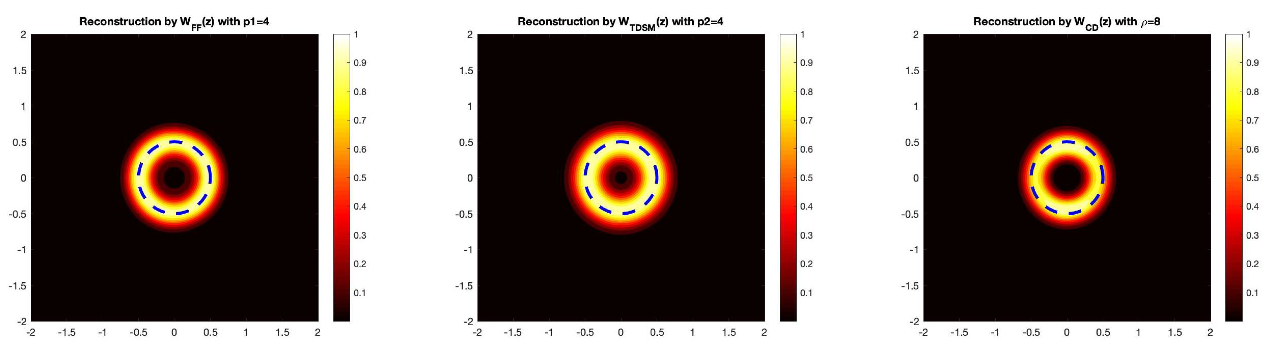
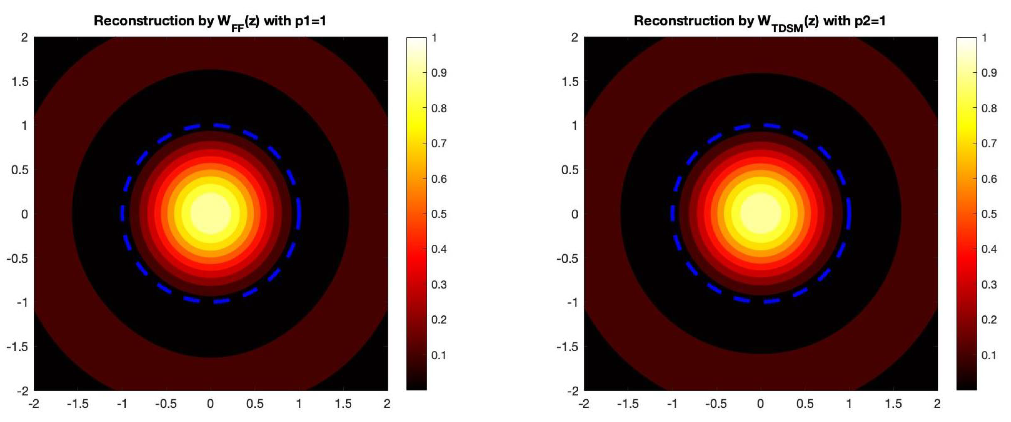
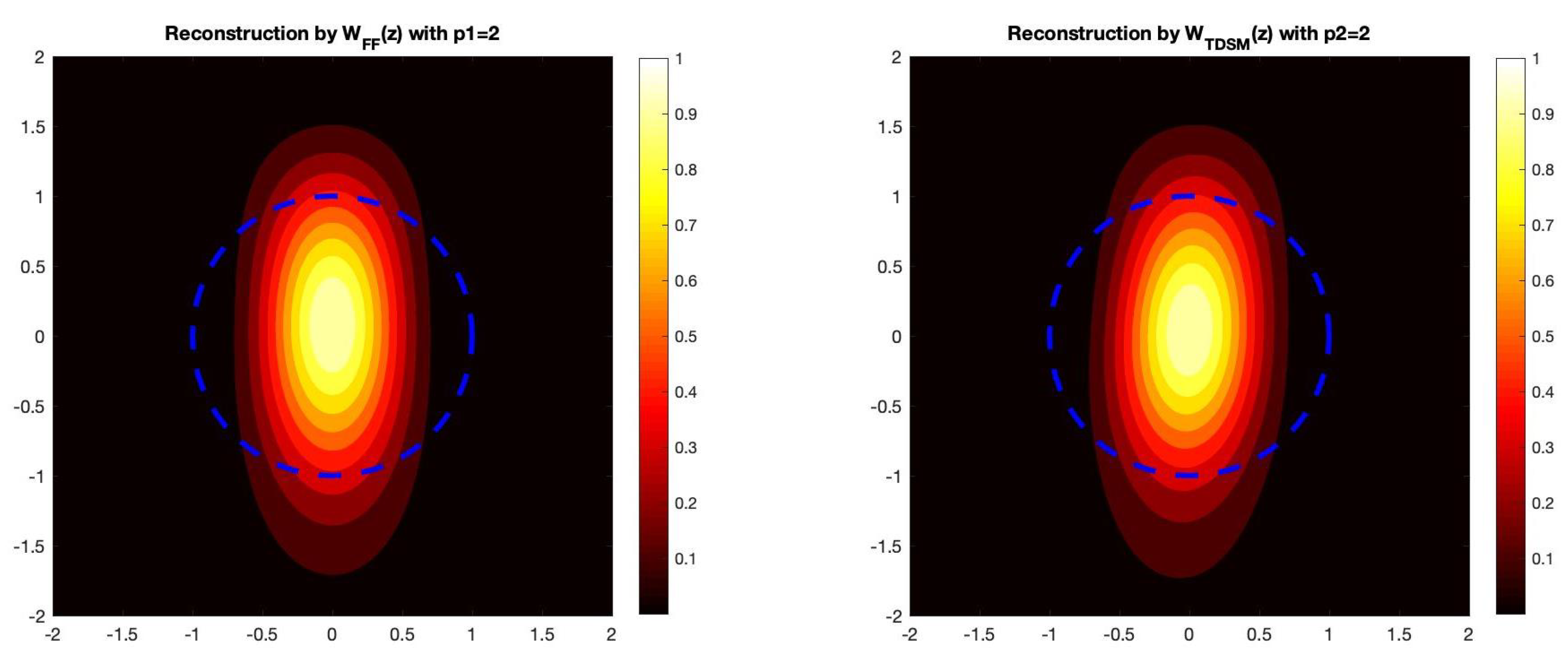
Example 1

(Circular Scatterer). For this example, we plot the imaging functionals to recover a circle. Therefore, we have that the radial function describing the scatterer is given by $r\left(\theta \right)=0.5$. Here, we take the wave number $k=4$ as well as the parameters $p1=p2=4$ and $\rho =8$. The dotted line represents the actual boundary of the circular obstacle in Figure 1.

Example 2

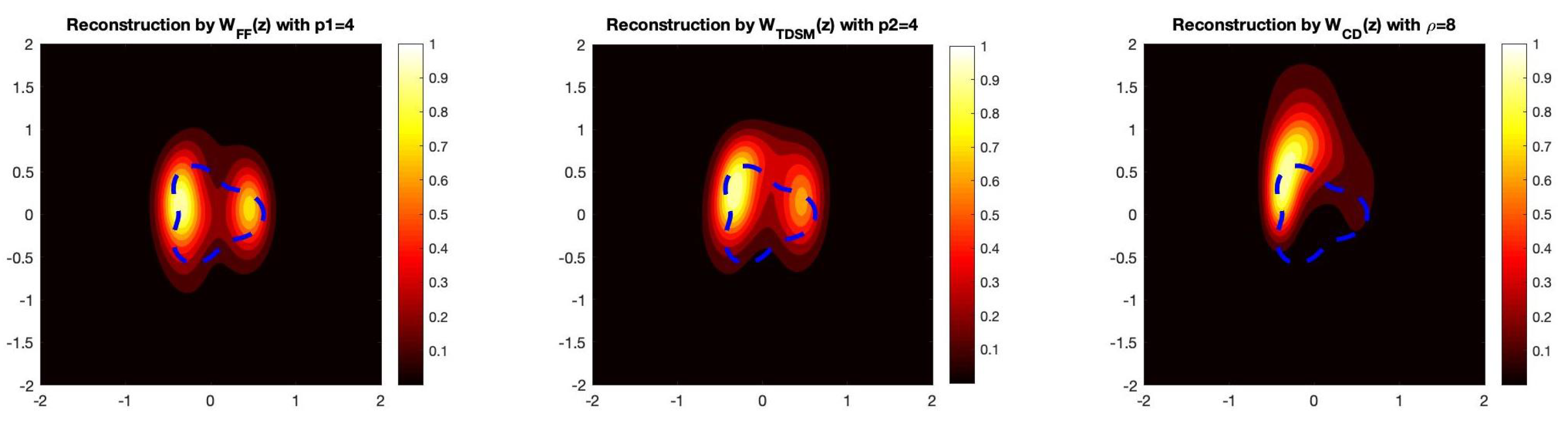
(Acorn-Shaped Scatterer). Now, we present a numerical example for recovering an acorn-shaped obstacle. Here, the radial function describing the scatterer is given by

$$r\left(\theta \right)=0.25\left(2+0.5cos\left(3\theta \right)\right).$$

For this example, we again take the wave number $k=4$ as well as $p1=p2=4$ and $\rho =8$. The dotted line represents the actual boundary of the acorn-shaped obstacle in Figure 2.

Example 3

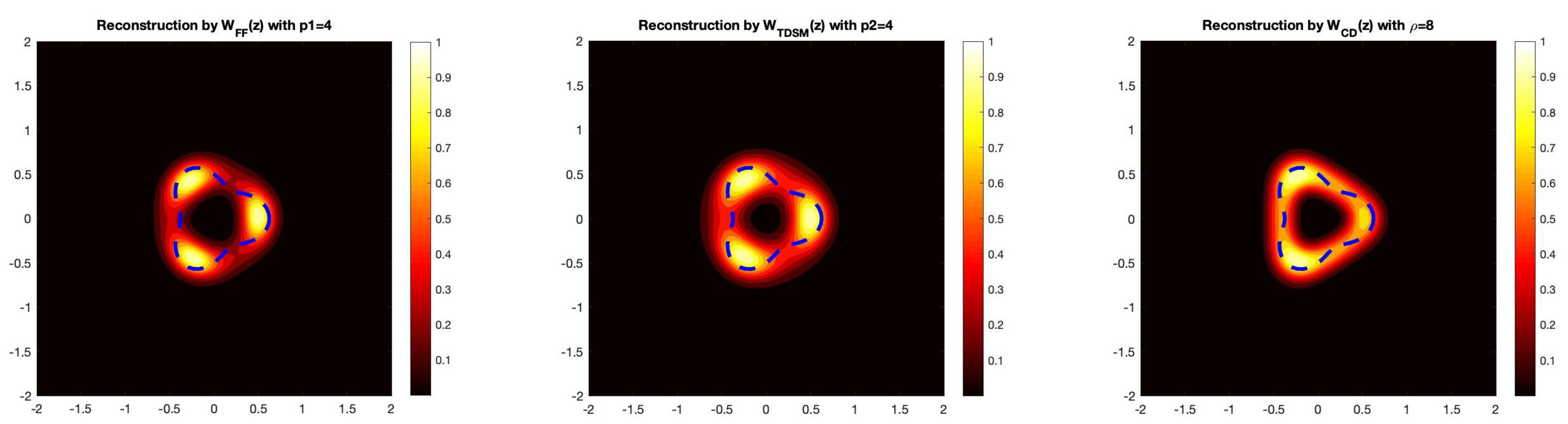
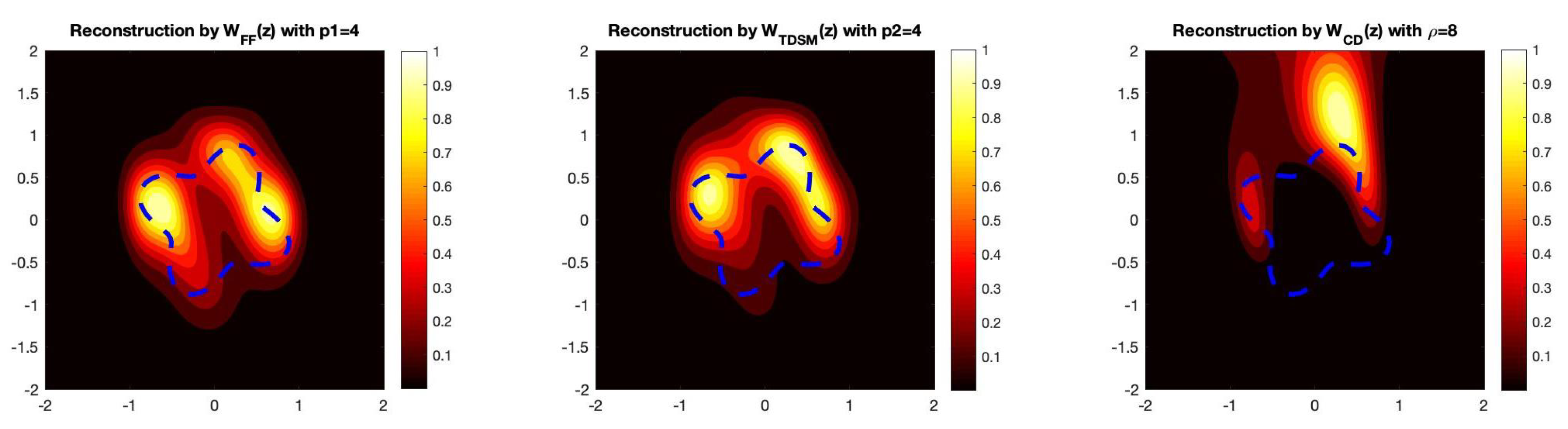
(Flower-Shaped Scatterer). Now, we present a numerical reconstruction for a flower-shaped obstacle, where the radial function is given by the following:

$$r\left(\theta \right)=0.75\left(1-0.25sin\left(4\theta \right)\right).$$

For this example, we again take the wave number $k=4$ as well as $p1=p2=4$ and $\rho =8$. The dotted line represents the actual boundary of the flower-shaped obstacle in Figure 3.

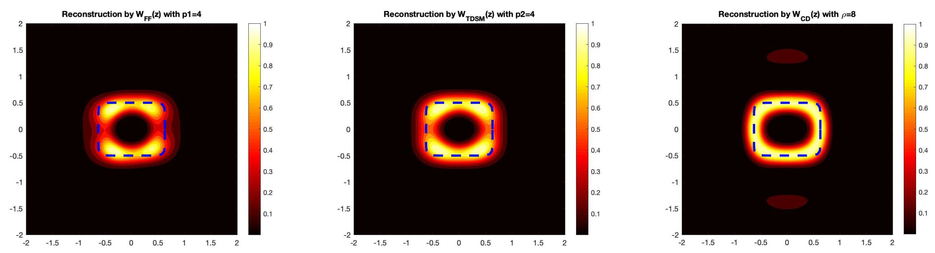
Example 4

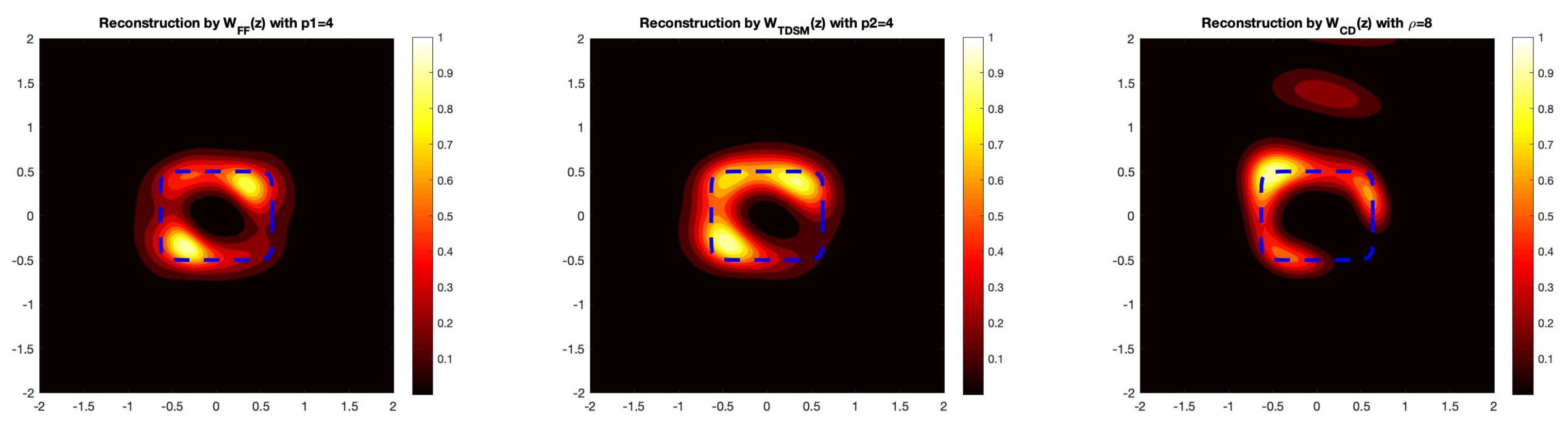
(Rounded-Square Scatterer). Now, we present a numerical reconstruction for a rounded square-shaped obstacle, where the radial function is given by the following:

$$r\left(\theta \right)=0.5{\left({|sin\left(\theta \right)|}^{10}+\frac{1}{10}{|cos\left(\theta \right)|}^{10}\right)}^{-1/10}.$$

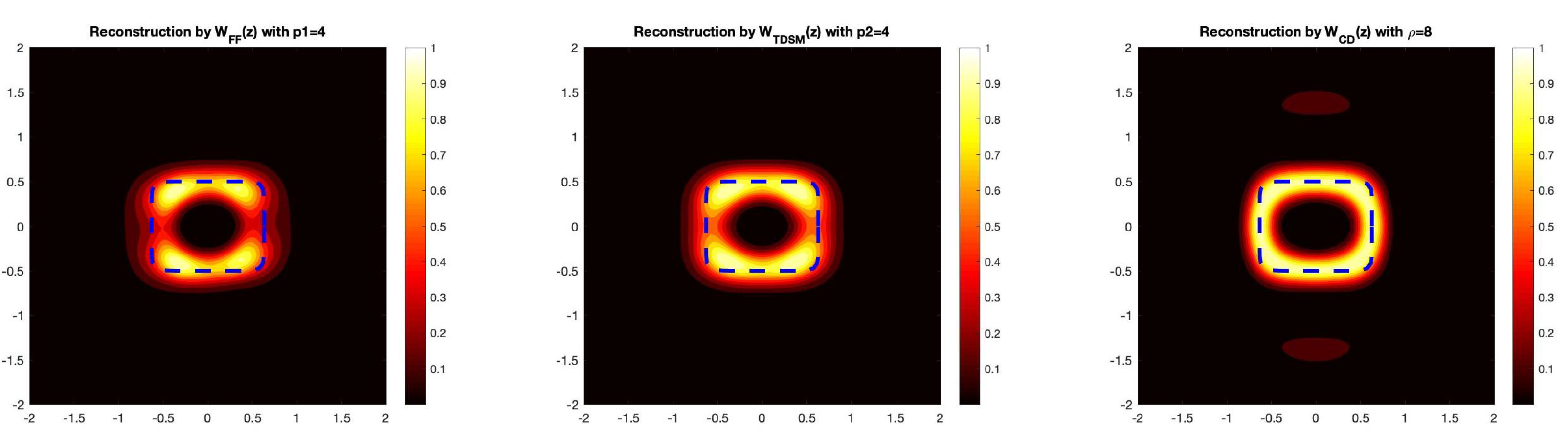
For this example, we again take the wave number $k=4$ as well as $p1=p2=4$ and $\rho =8$. The dotted line represents the actual boundary of the rounded-square in the figures. Here, we provide the reconstruction for two different noises levels in Figure 4 and Figure 5.

In the presented examples, we see that each imaging functional is stable with noise added to the data. This was noticed in [4], where large amounts of noise were added to the data, which do not seem to affect the reconstruction much. As we see in Figure 4 and Figure 5, there is little to no difference in the reconstructions when the noise level is increased. We also see that the reconstructions are similar in many cases, which is due to the fact that with the choice of parameters, we have that the three imaging functionals should have the same decay rate as $\mathrm{dist}(z,D)\to \infty$. Next, we present two examples with partial aperture data. Notice that the imaging functionals discussed here require full aperture data on the measurement surface $\Gamma$.

Example 5

(Partial Aperture Data for the Rounded-Square). Here, we provide two examples of reconstructing the rounded-square shaped obstacle with partial aperture data. Again, we take the wave number $k=4$ as well as $p1=p2=4$ and $\rho =8$, where we use the imaging functionals with data only given on $3/4$ and $1/2$ of the measurement surface.

In Figure 6 and Figure 7, we see that $W_{\mathrm{FF}}\left(z\right)$ and $W_{\mathrm{TDSM}}\left(z\right)$ seem to give better reconstructions than $W_{\mathrm{CD}}\left(z\right)$ for partial aperture data. Recently, in [24,25], some data completion methods were used to compute the missing scattering data, which were then used by a qualitative method to recover the scatterer. Applying these data completion methods can possibly be employed to provide better reconstructions with partial aperture data. Additionally, to derive a theoretically valid estimate for the imaging functions with partial aperture data, one should be able to use Theorem 4.1 in [26].

We now wish to provide further evidence that the imaging functionals $W_{\mathrm{FF}}\left(z\right)$ and $W_{\mathrm{TDSM}}\left(z\right)$ provide better reconstructions with partial data. To this end, we provide two more examples for the acorn- and flower-shaped scattering obstacles, using $1/2$ partial aperture data. Again, we plot all three functionals studied in the previous sections.

Example 6

(Partial Aperture Data for Non Convex Scatterer). In order to show that the imaging functionals $W_{\mathrm{FF}}\left(z\right)$ and $W_{\mathrm{TDSM}}\left(z\right)$ provide better reconstructions with partial data, we provide two more examples with $1/2$ partial aperture data, i.e., measurements only taken on ${\theta }_j\in [0,\pi )$. As in the other examples, we take the wave number $k=4$ as well as $p1=p2=4$ and $\rho =8$, where we recover the acorn- and flower-shaped obstacles.

As we see in Figure 8 and Figure 9, the imaging functionals $W_{\mathrm{FF}}\left(z\right)$ and $W_{\mathrm{TDSM}}\left(z\right)$ still outperform $W_{\mathrm{CD}}\left(z\right)$. Therefore, in the case of partial aperture data, the post-processing step of transforming the near-field data into far-field data is advantageous. This is especially useful for recovering non-convex shapes, where the non-convex part of the boundary is in the shadow region (i.e., where measurements are not given). We see this numerically in the case of the acorn- and flower-shaped obstacles that these functionals provide favorable reconstructions, even in the shadow region.

Example 7

(‘3D’ Reconstruction of the Unit Sphere). For completeness, we provide an example of reconstructing the unit sphere centered at the origin, using the imaging functionals $W_{\mathrm{FF}}\left(z\right)$ and $W_{\mathrm{TDSM}}\left(z\right)$. Here, we assume that $\Gamma =\partial B(0;R)$ with $R=5$ in three dimensions. In order to compute the scattered field $u^s$, we use the following formula (see, for example, Chapter 2 of [27]):

$$u^s(x,y)=-\sum _{n=0}^{\infty }(2n+1)\frac{h_n^{\left(1\right)}\left(5k\right)}{h_n^{\left(1\right)}\left(k\right)}{\int }_{{\mathbb{S}}^2}\Phi (\widehat{w},y)L_n\left(\widehat{\omega }·\widehat{x}\right)\mathrm{d}s\left(\widehat{w}\right).$$

Here, $L_n$ is the Legendre polynomial of degree n, and $h_n^{\left(1\right)}$ is the first-kind spherical Hankel function of the order n. The vectors on the unit sphere $\widehat{w}$ and $\widehat{x}$ are given by the following:

$$\widehat{w}={\left(sin\left({\theta }_w\right)cos\left({\varphi }_w\right),sin\left({\theta }_w\right)sin\left({\varphi }_w\right),cos\left({\theta }_w\right)\right)}^{\top }$$

as well as the following:

$$\widehat{x}={\left(sin\left({\theta }_x\right)cos\left({\varphi }_x\right),sin\left({\theta }_x\right)sin\left({\varphi }_x\right),cos\left({\theta }_x\right)\right)}^{\top }$$

with azimuthal angle $\theta \in [0,\pi )$ and polar angle $\varphi \in [0,2\pi )$. In this example, we recover the projection of the unit sphere in ${\mathbb{R}}^2$ (i.e., azimuthal angle $\theta =\pi /2$) by using the approximation of the near-field data as follows:

$$u^s(x_i,y_j)\approx -\sum _{n=0}^{10}(2n+1)\frac{h_n^{\left(1\right)}\left(5k\right)}{h_n^{\left(1\right)}\left(k\right)}{\int }_{{\mathbb{S}}^2}\Phi (\widehat{w},y_j)L_n(\widehat{\omega }·{\widehat{x}}_i)\mathrm{d}s\left(\widehat{w}\right).$$

Here, the points $x_i,y_j\in \partial B(0;R)$ with $R=5$ are given by $x_i=5{\widehat{x}}_i$ with the following:

$${\widehat{x}}_i={\left(cos\left({\varphi }_{x_i}\right),sin\left({\varphi }_{x_i}\right),0\right)}^{\top }\mathrm{and}{y}_j=5{\left(cos({\varphi }_{y_j}),sin({\varphi }_{y_j}),0\right)}^{\top }$$

where ${\varphi }_{x_i},{\varphi }_{y_j}\in [0,2\pi )$ are 64 equally spaced points. In order to compute the integrals, we first write them in spherical coordinates such that the following holds:

$${\int }_{{\mathbb{S}}^2}F\left(\widehat{w}\right)\mathrm{d}s\left(\widehat{w}\right)={\int }_0^{2\pi }{\int }_0^{\pi }F({\theta }_w,{\varphi }_w)sin\left({\theta }_w\right)\mathrm{d}{\theta }_w\mathrm{d}{\varphi }_w.$$

Then, to numerically approximate the integrals, we use the integral2 command in MATLAB. Since we have projected the data into two spacial dimensions, we can employ the method used for the previous examples. We take the wave number $k=1$ as well as $p1=p2=1$ in this example.

Example 8

(Partial Aperture Data for the Unit Sphere). For this example, we consider recovering the projection of the unit sphere in ${\mathbb{R}}^2$ with partial aperture data. Here, we assume that there are sources and receivers only on the upper half of the collection curve. To this end, we again use the method discussed in the previous example to compute the scattered field. Therefore, we have the approximated scattered field $u^s(x_i,y_j)$ where the points $x_i,y_j\in \partial B(0;R)$ are given by the following:

$$x_i=5{\left(cos\left({\varphi }_{x_i}\right),sin\left({\varphi }_{x_i}\right),0\right)}^{\top }\mathrm{and}{y}_j=5{\left(cos({\varphi }_{y_j}),sin({\varphi }_{y_j}),0\right)}^{\top }$$

where ${\varphi }_{x_i},{\varphi }_{y_j}\in [0,\pi )$ are 32 equally spaced points. For this example, we take the wave number $k=1$ as well as $p1=p2=2$.

Again, we see that the functionals with the far-field transformations are able to recover the obstacle even with ‘3D’ measurements given in Figure 10 and Figure 11. Additionally, notice that there is little to no difference in the reconstruction when one has a substantial amount of noise in the data. Lastly, we see that the imaging functional gives favorable reconstruction for ‘3D’ data with partial aperture data given by Figure 12.

6. Conclusions

In this paper, we have developed new direct sampling methods for near-field measurements. We focused on the case where the scatterer is a sound-soft obstacle, but just as in [3], we see that these imaging functionals should work for other types of scatterers. This is one of the main advantages of direct/qualitative reconstruction methods, but these methods do require full aperture data for their theoretical justification. Our numerical experiments seem to suggest that the imaging functionals derived by a far-field transformation provide reasonable results with partial aperture data. A direction in which this research can progress is to develop theoretical justification for the resolution analysis for new direct sampling methods with partial aperture data. Just as in [28,29], one can study the problem with multi-frequency data, which can often help reduce the amount of sources and receivers. One would need to factorize the corresponding multi-frequency data operator as is done in [30].

References

- Colton, D.; Kirsch, A. A simple method for solving inverse scattering problems in the resonance region. Inverse Probl. 1996, 12, 383–393. [Google Scholar] [CrossRef]
- Harris, I.; Kleefeld, A. Analysis of new direct sampling indicators for far-field measurements. Inverse Probl. 2019, 35, 054002. [Google Scholar] [CrossRef]
- Harris, I.; Nguyen, D.-L.; Nguyen, T.-P. New direct and orthogonality type sampling methods for near field measurements. arXiv 2016, arXiv:2107.08138. [Google Scholar]
- Liu, X. A novel sampling method for multiple multiscale targets from scattering amplitudes at a fixed frequency. Inverse Probl. 2017, 33, 085011. [Google Scholar] [CrossRef] [Green Version]
- Chow, Y.T.; Ito, K.; Liu, K.; Zou, J. Direct Sampling Method for Diffusive Optical Tomography. SIAM J. Sci. Comput. 2015, 37, A1658–A1684. [Google Scholar] [CrossRef]
- Chow, Y.T.; Ito, K.; Zou, J. A direct sampling method for electrical impedance tomography. Inverse Probl. 2014, 30, 095003. [Google Scholar] [CrossRef] [Green Version]
- Chow, Y.T.; Ito, K.; Zou, J. A Time-Dependent Direct Sampling Method for Recovering Moving Potentials in a Heat Equation. SIAM J. Sci. Comput. 2018, 40, A2720–A2748. [Google Scholar] [CrossRef]
- Hald, J. Patch near-field acoustical holography using a new statistically optimal method. In Proceedings of the Inter-Noise 2003, Jeju, Korea, 23–26 August 2003. [Google Scholar]
- Maynard, D.; Williams, E.G.; Lee, Y. Nearfield acoustic holography: I. Theory of generalized holography and the development of NAH. J. Acoust. Soc. Am. 1985, 78, 1395–1413. [Google Scholar] [CrossRef]
- Scholte, R. Fourier Based High-Resolution Near-Field Sound Imaging; Technische Universiteit Eindhoven: Eindhoven, The Netherlands, 2008. [Google Scholar] [CrossRef]
- Cakoni, F.; Colton, D.; Haddar, H. Inverse Scattering Theory and Transmission Eigenvalues; CBMS Series; SIAM Publications: Philadelphia, PA, USA, 2016. [Google Scholar]
- Kirsch, A.; Grinberg, N. The Factorization Method for Inverse Problems; Oxford University Press: Oxford, UK, 2008. [Google Scholar]
- Cakoni, F.; Haddar, H.; Lechleiter, A. On the factorization method for a far field inverse scattering problem in the time domain. SIAM J. Math. Anal. 2019, 51, 854–872. [Google Scholar] [CrossRef] [Green Version]
- Guo, J.; Nakamura, G.; Wang, H. The factorization method for recovering cavities in a heat conductor. arXiv 2019, arXiv:1912.11590. [Google Scholar]
- Kirsch, A. Characterization of the shape of the scattering obstacle by the spectral data of the far field operator. Inverse Probl. 1998, 14, 1489–1512. [Google Scholar] [CrossRef]
- Chen, J.; Chen, Z.; Huang, G. Reverse time migration for extended obstacles: Acoustic waves. Inverse Probl. 2013, 29, 085005. [Google Scholar] [CrossRef] [Green Version]
- Colton, D.; Kress, R. Inverse Acoustic and Electromagnetic Scattering Theory, 3rd ed.; Applied Mathematical Sciences; Springer: New York, NY, USA, 2013; Volume 93. [Google Scholar]
- Hu, G.; Yang, J.; Zhang, B.; Zhang, H. Near-field imaging of scattering obstacles with the factorization method. Inverse Probl. 2014, 30, 095005. [Google Scholar] [CrossRef] [Green Version]
- McLean, W. Strongly Elliptic Systems and Boundary Integral Equation; Cambridge University Press: Cambridge, UK, 2000. [Google Scholar]
- Brezis, H. Functional Analysis, Sobolev Spaces and Partial Differential Equations; Springer: New York, NY, USA, 2011. [Google Scholar]
- Evans, L. Partial Differential Equation, 2nd ed.; AMS: Providence, RI, USA, 2010. [Google Scholar]
- Kirsch, A. An Introduction to the Mathematical Theory of Inverse Problems, 2nd ed.; Springer: New York, NY, USA, 2011. [Google Scholar]
- Leem, K.H.; Liu, J.; Pelekanos, G. Two direct factorization methods for inverse scattering problems. Inverse Probl. 2018, 34, 125004. [Google Scholar] [CrossRef]
- Dou, F.; Liu, X.; Meng, S.; Zhang, B. Data completion algorithms and their applications in inverse acoustic scattering with limited-aperture backscattering data. arXiv 2021, arXiv:2106.11101. [Google Scholar]
- Liu, X.; Sun, J. Data recovery in inverse scattering: From limited-aperture to full-aperture. J. Comput. Phys. 2019, 386, 350–364. [Google Scholar] [CrossRef]
- Park, W.-K. Multi-frequency subspace migration for imaging of perfectly conducting, arc-like cracks in full- and limited view inverse scattering problems. J. Comput. Phys. 2015, 283, 52–80. [Google Scholar] [CrossRef] [Green Version]
- Kirsch, A.; Hettlich, F. The Mathematical Theory of Time Harmonic Maxwell’s Equations. Expansion-, Integral-, and Variational Methods; Applied Mathematical Sciences; Springer: New York, NY, USA, 2015. [Google Scholar]
- Alzaalig, A.; Hu, G.; Liu, X.; Sun, J. Fast acoustic source imaging using multi-frequency sparse data. Inverse Probl. 2020, 36, 025009. [Google Scholar] [CrossRef] [Green Version]
- Arens, T.; Ji, X.; Liu, X. Inverse electromagnetic obstacle scattering problems with multi-frequency sparse backscattering far field data. Inverse Probl. 2020, 36, 105007. [Google Scholar] [CrossRef]
- Griesmaier, R.; Schmiedecke, C. A Factorization Method for Multifrequency Inverse Source Problems with Sparse Far Field Measurements. SIAM J. Imaging Sci. 2017, 10, 2119–2139. [Google Scholar] [CrossRef]
Figure 1.
The reconstruction of the circular obstacle by the three direct sampling imaging functionals. In this example, we take , which corresponds to a 5% noise level.
Figure 2.
The reconstruction of the acorn-shaped obstacle by the three direct sampling methods. In this example, we take , which corresponds to a 5% noise level.
Figure 3.
The reconstruction of the flower-shaped obstacle by the three direct sampling methods. In this example, we take , which corresponds to a 5% noise level.
Figure 4.
The reconstruction of the rounded square by the three direct sampling imaging functionals. In this example, we take , which corresponds to a 5% noise level.
Figure 5.
The reconstruction of the rounded square by the three direct sampling imaging functionals. In this example, we take , which corresponds to a 25% noise level.
Figure 6.
The reconstruction of the rounded square with partial aperture data, i.e., measurements only taken on . In this example, we take which corresponds to a 5% noise level.
Figure 7.
The reconstruction of the rounded square with partial aperture data, i.e., measurements only taken on . In this example, we take , which corresponds to a 5% noise level.
Figure 8.
The reconstruction of the acorn-shaped obstacle with partial aperture data. In this example, we take , which corresponds to a 5% noise level.
Figure 9.
The reconstruction of the flower-shaped obstacle with partial aperture data. In this example, we take , which corresponds to a 5% noise level.
Figure 10.
The reconstruction of the unit sphere by the direct sampling imaging functionals. In this example, we take , which corresponds to a 5% noise level.
Figure 11.
The reconstruction of the unit sphere by the direct sampling imaging functionals. In this example, we take , which corresponds to a 25% noise level.
Figure 12.
The reconstruction of the unit sphere with partial aperture data by the imaging functionals. In this example, we take , which corresponds to a 5% noise level.
Publisher’s Note: MDPI stays neutral with regard to jurisdictional claims in published maps and institutional affiliations. |
© 2021 by the author. Licensee MDPI, Basel, Switzerland. This article is an open access article distributed under the terms and conditions of the Creative Commons Attribution (CC BY) license (https://creativecommons.org/licenses/by/4.0/).
Share and Cite
MDPI and ACS Style
Harris, I. Direct Sampling for Recovering Sound Soft Scatterers from Point Source Measurements. Computation 2021, 9, 120. https://0-doi-org.brum.beds.ac.uk/10.3390/computation9110120
AMA Style
Harris I. Direct Sampling for Recovering Sound Soft Scatterers from Point Source Measurements. Computation. 2021; 9(11):120. https://0-doi-org.brum.beds.ac.uk/10.3390/computation9110120
Chicago/Turabian StyleHarris, Isaac. 2021. "Direct Sampling for Recovering Sound Soft Scatterers from Point Source Measurements" Computation 9, no. 11: 120. https://0-doi-org.brum.beds.ac.uk/10.3390/computation9110120
Note that from the first issue of 2016, this journal uses article numbers instead of page numbers. See further details here.