Some Finite Difference Methods to Model Biofilm Growth and Decay: Classical and Non-Standard

Abstract

The study of biofilm formation is undoubtedly important due to micro-organisms forming a protected mode from the host defense mechanism, which may result in alteration in the host gene transcription and growth rate. A mathematical model of the nonlinear advection–diffusion–reaction equation has been studied for biofilm formation. In this paper, we present two novel non-standard finite difference schemes to obtain an approximate solution to the mathematical model of biofilm formation. One explicit non-standard finite difference scheme is proposed for biomass density equation and one property-conserving scheme for a coupled substrate–biomass system of equations. The nonlinear term in the mathematical model has been handled efficiently. The proposed schemes maintain dynamical consistency (positivity, boundedness, merging of colonies, biofilm annihilation), which is revealed through experimental observation. In order to verify the accuracy and effectiveness of our proposed schemes, we compare our results with those obtained from standard finite difference schemes and earlier known results in the literature. The proposed schemes (NSFD1 and NSFD2) show good performance. The NSFD2 scheme reveals that the processes of biofilm formation and nutritive substrate growth are intricately linked.

1. Introduction

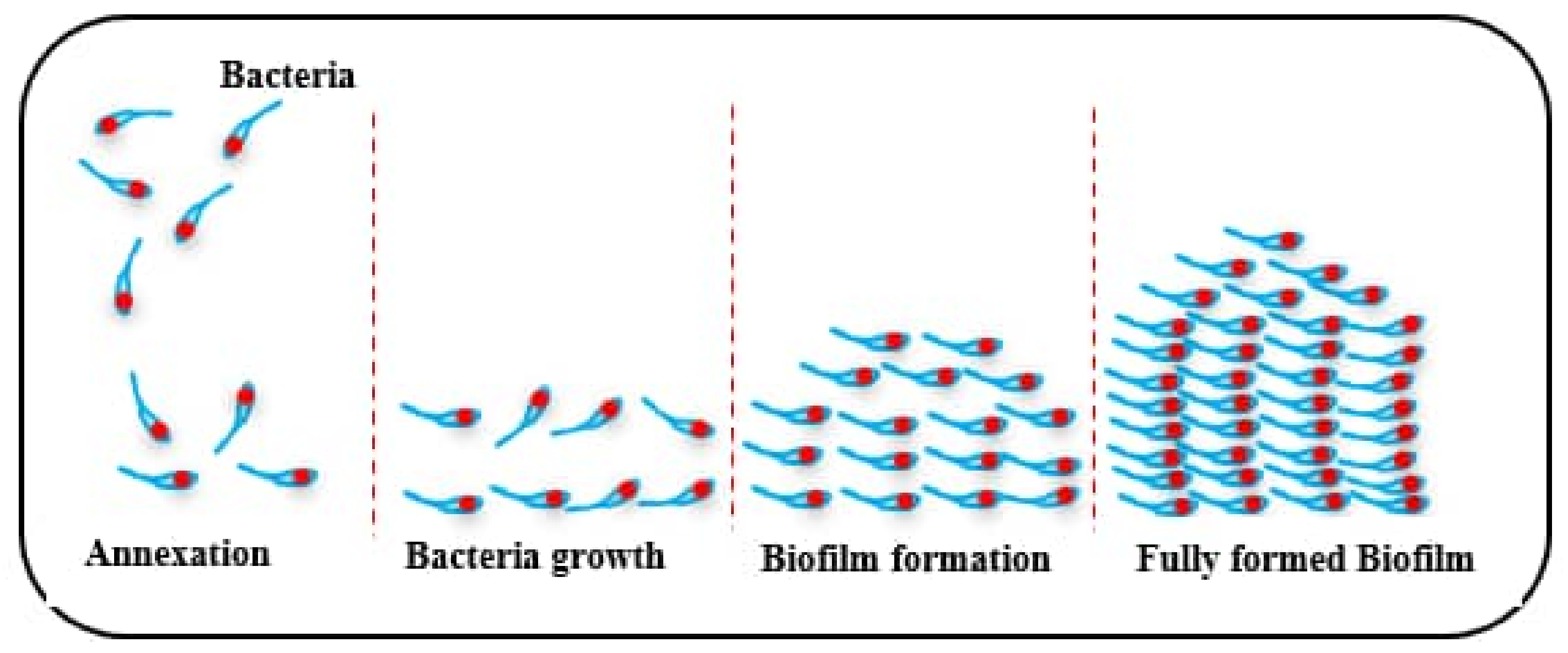
The word biofilm refers to aggregation of smaller organisms existing on a changing interface embedded in a polymeric matrix adhered to abiotic or biotic surfaces. Bacteria in biofilms grow in a protected environment, which improves their ability to survive in harsh conditions [1]. In general, preventing the formation of harmful biofilms is difficult due to their adaptability to growing in harsh conditions. Furthermore, one must recognize the difficulty of biofilm removal, as the bacteria that create the biofilm are more resistant to antimicrobial treatments and the host’s immune response. The formation of biofilm by bacteria is due to a coordinated mechanism called Quorum Sensing (QS) [1]. Biofilm formation takes place in connecting steps, which are as follows [2]:

• Formation of conditioning surface;
• The adhesion of bacteria to the conditioning surface;
• Bacterial growth at the surface;
• Biofilm formation begins after a quorum of bacteria has been reached;
• Expansion of the biofilm to a fully-developed state—see Figure 1.

A biofilm may occur on a wide range of surfaces, including tissues, glass, plastic, metal, wood, soil particles and food items. Factors that promote biofilm development include conditioning film, hydrodynamics, horizontal gene transfer, the substratum effect and quorum sensing. The importance of understanding biofilm formation cannot be over-emphasized due to its relevance in biology, medicine and other scientific research. To this end, many research works with the main objective of understanding biofilm formations have been conducted, among which are the works of Rittmann and McCarty [3] and Wanner and Gujer [4]. Nilsson et al. [5] probed the effect of changes in acylated homoserine lactone (AHL) concentration and investigated the possibility of biofilm formation using a mathematical model. Their model consists of a set of coupled ordinary differential equations (ODEs) in which the bacterial growth is modelled using the well-known logistic equation:

$$\left\{\begin{array}{c}{\displaystyle \frac{d{\eta }_{bc}}{dt}}=h\left(C_{bc}\right)N\left(t\right)-4\pi r_{bc}^{2}N{\left(t\right)}^{2/3}{\gamma }^{2/3}\hfill \\ {\displaystyle \frac{d{\eta }_{bf}}{dt}}={\Delta }_{bc}-\beta 4\pi r_{bc}^{2}N{\left(t\right)}^{2/3}{\gamma }^{2/3}(C_{bf}-C_w),\hfill \end{array}\right.$$

(1)

where ${\eta }_{bc}$ is the AHL inside a single bacterium cell, ${\eta }_{bf}$ is the AHL in the biofilm, $C_{bc}$ represents the concentration of AHL in the cell, $C_{bf}$ stands for the concentration of AHL in the biofilm, and $C_w$ is the concentration of AHL in the water phase. $N\left(t\right)={\displaystyle \frac{K}{1+\left(\frac{K}{N_o}-1\right)e^{-\rho t}}}$ is the number of bacteria, $r_{bc}$ denotes the radius of a single bacterium, $\gamma$ determines how densely the bacteria are packed, K is the number of bacteria in the stationary phase, $N_o$ stands for the initial number of bacteria at $t=0$, $\rho$ is the intrinsic growth rate and $\beta$ is the permeability parameter characteristic of the surface of the biofilm.

Readers are referred to the work of Nilsson et al. [5] for a full understanding of their study. The study concluded that the autoinduction of AHL and biofilm formation are highly interconnected. Many known mathematical models in the literature are represented in terms of partial differential equations (PDEs) with a nonlinear density-dependent diffusion reaction describing biofilm growth. Eberl et al. [6] presented a mathematical model of biofilm formation, which comprises two coupled partial differential equations, namely the biomass system and substrate nutrients, given by

$$\left\{\begin{array}{c}{\displaystyle \frac{\partial u\left(\mathbf{x}\right)}{\partial t}}={\Gamma }_1{\nabla }^{2}u\left(\mathbf{x}\right)-{\Gamma }_3{\displaystyle \frac{v\left(\mathbf{x}\right)u\left(\mathbf{x}\right)}{{\Gamma }_4+u\left(\mathbf{x}\right)}},\hfill \\ {\displaystyle \frac{\partial v\left(\mathbf{x}\right)}{\partial t}}={\Gamma }_2\nabla ·D\left(v\left(\mathbf{x}\right)\right)\nabla v\left(\mathbf{x}\right)-rv\left(\mathbf{x}\right)+{\Gamma }_5{\displaystyle \frac{v\left(\mathbf{x}\right)u\left(\mathbf{x}\right)}{{\Gamma }_4+u\left(\mathbf{x}\right)}},\hfill \\ D\left(v\left(\mathbf{x}\right)\right)={\displaystyle \frac{\delta v{\left(\mathbf{x}\right)}^{\lambda }}{{(1-v\left(\mathbf{x}\right))}^{\mu }}},\hfill \\ \mathrm{where}\lambda >0,\mu >0,\mathsf{\Omega }\times [0,T],\mathsf{\Omega }\in {\mathbb{R}}^d(d=1,2,3).\hfill \end{array}\right.$$

(2)

We note that $\nabla$ and ${\nabla }^2$ are the usual gradient and Laplacian operators and that u and v are the substrate nutrient and normalized density of biomass. The non-negative parameters in Equation (2), namely ${\Gamma }_1,{\Gamma }_2,{\Gamma }_3,{\Gamma }_4,{\Gamma }_5$ and r, are the substrate diffusion coefficient, biomass diffusion coefficient, maximum specific consumption rate, monod half saturation constant, maximum specific growth rate and biomass decay rate, respectively. The diffusion coefficient $D\left(v\right)$ is clearly written in terms of the biomass density. The term ${\Gamma }_2\nabla ·D\left(v\right)\nabla v$ makes the system of equations highly non-linear. The diffusion term in the substrate equation is represented as ${\Gamma }_1{\nabla }^{2}u$. The reaction rate terms written in Michaelis–Menten form are ${\Gamma }_3{\displaystyle \frac{vu}{{\Gamma }_4+u}}$ and ${\Gamma }_5{\displaystyle \frac{vu}{{\Gamma }_4+u}}$. $\mathbf{x}$ represents the vector of spatial variables x and y.

From the current literature, providing an exact solution to Equation (2) is still a daunting task. However, the analytical investigation of the existence, uniqueness and long term behaviour of the solution has been established; see the work of Efendiev et al. [7]. Eberl and his collaborators [6] constructed a finite difference discretizaton solution for Equation (2). The major drawback of their numerical scheme is that the scheme is computationally demanding and time consuming [8]. Eberl and Demaret [9] provided a non-classical finite difference scheme for the numerical solution to Equation (2) which preserves the condition of merging of two different colonies. The scheme preserves the non-negativity of the solution as established in [7]. Morales-Hernandez et al. [10] considered a limiting case, ${\Gamma }_1={\Gamma }_3={\Gamma }_5=0$ of Equation (2), which results in

$${\displaystyle \frac{\partial v}{\partial t}}={\Gamma }_2\nabla ·D\left(v\right)\nabla v+rv,$$

(3)

where $D\left(v\right)$ is defined as in Equation (2). The authors provided a recursive positivity-preserving finite difference scheme with bounded approximation. The M-matrix theorem was the cornerstone upon which the non-negativity of the solution was established. We note here the use of the stabilized bi-conjugate gradient method to obtain their solution. In addition, Moralez et al. [11] published a corrigendum to their work to shed more light on the subject matter. In a similar study, Sun et al. [12] designed a new non-standard finite difference scheme for Equation (3). The method shows reasonable behaviour and preserves the properties of the equation. However, the author mentioned the inconsistency of the method. Macias-Diaz et al. [8] solved Equation (3) using another explicit finite difference scheme. The non-standard finite difference scheme was employed by the authors to preserve the positivity of the solution. One major drawback of their method is the implicit implementation of their algorithm, which requires Newton’s method because of the presence of the nonlinear term. Sun et al. [13] investigated Equation (2) in its full form using a non-standard finite difference scheme and a classical upwind forward Euler finite difference scheme. They discussed the preservation of positivity and boundedness of the non-standard scheme. In addition, the authors considered four different cases of the problem: a mixed biological density constriction framework, mixed biological density developing framework, complex coupling system in which the density of the biological evolution process is increased at the first stage and then decreases and a mixed biological framework with discontinuous initial conditions and Dirichlet boundary conditions [13].

Balsa-Canto et al. [14] used the time discretization Crank Nicolson finite difference scheme with the Newton algorithm to study similar PDEs, as shown in Equation (2). The scheme is computationally fast, and the results obtained are in agreement with experimental results. Afsar-Ali et al. [15] employed the semi-implicit finite volume method to obtain a numerical solution to Equation (2) in a non-orthogonal grid; this is possible after the transformation of the governing equation to a non-curvilinear system. In other related studies, Duddu et al. [16] used the extended finite element method to computationally investigate the growth of biofilm. Bol et al. [17] theoretically investigated 3D biofilm detachment using the finite element method. We refer readers to the following studies for more work in this direction: Macias-Diaz et al. [18], Liao et al. [19] and Eberl [20] proposed another mathematical model which comprises four coupled partial differential equations and is an extension of Equation (2). Macias-Diaz [21] studied the modified mathematical model by constructing a positivity-preserving linear finite difference scheme, in contrast to the non-linear finite-difference scheme proposed by Eberl [20].

In another study, Fredrick et al. [22] used a mathematical model to study the relationship between quorum sensing extracellular polymeric substance production and biofilm formation. The emerging equation is a reaction–diffusion equation, and the absence of an analytical solution led to the computational investigation of the model. Appadu [23] investigated the performance of the unconditionally positive finite difference scheme for a linear advection–diffusion–reaction equation under various advection, diffusion and reaction regimes. Recently, Jornet [24] proposed a mathematical model of biofilm formation on a medical implant using a new growth model rather than the logistic growth model; the resulting differential equation is the Allen–Cahn partial differential equation.

The novelty of this work is the design of a novel structure-preserving (positivity, boundedness, merging of colonies, biofilm annihilation) finite-difference scheme to approximate the full and limiting cases of Equation (2), which describes the growth/decay of a microbial colony. We compare the performance of our scheme against earlier known work in the literature and with the classical finite difference scheme.

2. Organization of the Paper

The structure of this paper is briefly outlined here. In Section 3, we describe in detail the mathematical model governing the nutritive substrate of the non-linear diffusion–reaction equation in bio-film formations. Furthermore, the substantiate conditions of the existence and uniqueness of the solution are provided to shed more light. Section 4 contains an analysis of the mathematical model and discretization of our domain. In Section 5, we present two novel finite difference techniques for the biomass-independent equation and show the preservation of positivity and boundedness. We graphically examine the performance of our proposed scheme and provide a discussion in Section 6. In Section 7, we present a property-preserving finite difference scheme for a coupled substrate–biomass equation. The performance of the scheme is subjected to examination in Section 8. Finally, our conclusion and the significance of the present study are elaborated in Section 9.

3. Mathematical Model

The processes that govern mass transport, biofilm accumulation and organic constituent biotransformation are inextricably linked. Consider a spatially structured bacterial biofilm with a density-dependent diffusion–reaction equation given by (2); i.e.,

$$\left\{\begin{array}{c}{\displaystyle \frac{\partial u\left(\mathbf{x}\right)}{\partial t}}={\Gamma }_1{\nabla }^{2}u\left(\mathbf{x}\right)-{\Gamma }_3{\displaystyle \frac{v\left(\mathbf{x}\right)u\left(\mathbf{x}\right)}{{\Gamma }_4+u\left(\mathbf{x}\right)}},\mathsf{\Omega }\times [0,T],\mathsf{\Omega }\in {\mathbb{R}}^d(d=1,2,3),\hfill \\ {\displaystyle \frac{\partial v\left(\mathbf{x}\right)}{\partial t}}={\Gamma }_2\nabla ·D\left(v\left(\mathbf{x}\right)\right)\nabla v\left(\mathbf{x}\right)-rv\left(\mathbf{x}\right)+{\Gamma }_5{\displaystyle \frac{v\left(\mathbf{x}\right)u\left(\mathbf{x}\right)}{{\Gamma }_4+u\left(\mathbf{x}\right)}},\hfill \\ D\left(v\left(\mathbf{x}\right)\right)={\displaystyle \frac{\delta v{\left(\mathbf{x}\right)}^{\lambda }}{{(1-v\left(\mathbf{x}\right))}^{\mu }}},\lambda >0,\mu >0.\hfill \end{array}\right.$$

with boundary and initial condition

$$\left\{\begin{array}{c}u(\mathbf{x},t)=1,v(\mathbf{x},t)=0,\forall \mathbf{x}\in \partial \mathsf{\Omega },t\ge 0,\hfill \\ u(\mathbf{x},0)=u_0\left(\mathbf{x}\right),v(\mathbf{x},0)=v_0\left(\mathbf{x}\right).\hfill \end{array}\right.$$

(4)

The boundary condition can either be homogeneous Dirichlet or homogeneous Neumann [8]. All variables and parameters are defined in Equation (2). The following results guarantee the existence and uniqueness of non-negativity and boundedness of solutions for Equations (2) and (3).

Theorem 1.

If the initial data $u_0$ and $v_0$ satisfy the conditions

• $u_0\in L^{\infty }\left(\mathsf{\Omega }\right) \cap J^1\left(\mathsf{\Omega }\right)$ and $0\le u_0\left(\mathit{x}\right)\le 1$ for every $\mathit{x}\in \mathsf{\Omega }$
• $v_0\in L^{\infty }\left(\mathsf{\Omega }\right)$ and $G\left(v_0\right) \in J_0^1\left(\mathsf{\Omega }\right)$
• $v_0\left(\mathit{x}\right)\ge 0$ for every $\mathit{x}\in \mathsf{\Omega }$ and $\left|\right|v_0{\left|\right|}_{L^{\infty }\left(\mathsf{\Omega }\right)}<1$,

where

$$G\left(v\right)={\int }_0^v{\displaystyle \frac{s^{\lambda }}{{(1-s)}^{\mu }}}ds,0\le v<1,$$

(5)

then Equation (2) has a unique solution subject to suitable conditions in Equation (4) obeying the following properties:

• $u,v\in L^{\infty }\left(\mathsf{\Omega }\times {\mathbb{R}}^{+}\right) \cap C\left(L^2\left(\mathsf{\Omega }\right),[0,\infty )\right)$
• $u,G\left(v\right)\in L^{\infty }\left(J^1\left(\mathsf{\Omega }\right)\times {\mathbb{R}}^{+}\right)$$\cap C\left(L^2\left(\mathsf{\Omega }\right),[0,\infty )\right)$
• $0\le u(\mathit{x},t),v(\mathit{x},t)\le 1$ for every $(\mathit{x},t)\in \mathsf{\Omega }\times {\mathbb{R}}^{+}$ and ${\left|\right|v\left|\right|}_{L^{\infty }(\mathsf{\Omega }\times {\mathbb{R}}^{+})}<1$.

Remark 1.

Theorem 1 was established using several mathematical propositions, corollaries and assumptions such as continuity, triangle inequality, Gronwall inequality and the boundedness property. We refer the reader to the work of Efendiev et al. [7] for the rigorous proof of Theorem 1.

A plausible numerical solution for Equation (2) must satisfy the following experimental conditions:

• Existence of a sharp front of biomass at the fluid to solid transition;
• Biomass spreading is more important when a particular maximum density is reached and biomass density cannot exceed a certain maximum;
• Reaction process dynamics facilitate biomass production, and partial heterogeneities in a biofilm come from environmental conditions;
• Biomass movement should be in agreement with hydrodynamics and nutrient transfer/consumption models.

4. Model Analysis

We consider two problems from Equation (2), which are

• The biomass-independent equation with three cases (Problem 1);
• The coupled substrate–biomass system of equations with two cases (Problem 2). Problem 2 is explained in Section 7.

The biomass-independent diffusion–reaction equation is given by (see [8])

$${\displaystyle \frac{\partial v}{\partial t}}=\nabla ·D\left(v\right)\nabla v+rv,t\in {\mathbb{R}}^{+},v=v(x,y,t).$$

(6)

with the initial condition

$$v(x,y,0)=\varphi (x,y),$$

(7)

where $\varphi (x,y)$ is a given function defined and bounded between $[0,1]$. Boundary conditions are either homogeneous Dirichlet or homogeneous Neumann. From experimental observation, if the homogeneous Neumann conditions are specified somewhere on the boundary data, the solution v reaches its maximum density 1 almost everywhere at finite time t. If the boundary conditions are of Dirichlet type, then $v=0$ everywhere; v remains non-negative and lies below the maximum density 1 for all $t>0$.

Re-writing Equation (6) in an alternative way gives

$${\displaystyle \frac{\partial v}{\partial t}}=D^{\prime }\left(v\right)\left({\left({\displaystyle \frac{\partial v}{\partial x}}\right)}^2+{\left({\displaystyle \frac{\partial v}{\partial y}}\right)}^2\right)+D\left(v\right)\left({\displaystyle \frac{{\partial }^{2}v}{\partial x^2}}+{\displaystyle \frac{{\partial }^{2}v}{\partial y^2}}\right)+rv.$$

(8)

We first describe the finite-difference approximation for each term in Equation (8) before coupling them together.

Before considering the derivation of our novel scheme, our numerical discretization and estimation tools are given below.

Let $a,b,c$ and d be real numbers such that $a<b$ and $c<d$. An open rectangle domain can be defined as $\mathsf{\Omega }=(a,b)\times (c,d)$ in ${\mathbb{R}}^2$. We consider a bounded domain interval of $0\le x,y\le 1$. Hence, regular equal grid spacings in the spatial domain $[a,b],[c,d]$ and time domain $[0,T]$ are

$$\begin{array}{l}\hspace{1em}\hspace{1em}\hspace{1em}a=x_1<x_2<x_3<x_4<\cdots <x_{N+1}=b,\\ \hspace{1em}\hspace{1em}\hspace{1em}c=y_1<y_2<y_3<y_4<\cdots <x_{M+1}=d,\\ \mathrm{and}\\ \hspace{1em}\hspace{1em}\hspace{1em} 0=t_1<t_2<t_3<t_4<\cdots <t_{W+1}=T.\end{array}$$

(9)

With the above spatial variables, the intervals along x and y axes are divided into $(N+1)$ and $(M+1)$ nodes, respectively, while the time interval $[0,T]$ can be divided into $(W+1)$ grid points. We define our grid points $(x_i,y_j,t_n)$ as

$$\begin{array}{c}\hfill x_i=(i-1)h_x,i=1,2,3,...,N+1\mathrm{with}{h}_x={\displaystyle \frac{b-a}{N}},\\ \hfill y_j=(j-1)h_y,j=1,2,3,...,M+1\mathrm{with}{h}_y={\displaystyle \frac{d-c}{M}},\\ \hfill t_n=(n-1)k,n=1,2,3,...,W+1\mathrm{with}k={\displaystyle \frac{T}{W}},\end{array}$$

(10)

and $(N-1)h_x=(M-1)h_y=1$, $(W-1)k=T$. For convenience, throughout this work, we take $h_x=h_y=h$.

Since an analytical solution is not obtainable, we use dynamical consistency as well as the rate of convergence in order to gauge the numerical performance of our schemes. The rate of convergence formula is computed using [25]

$$R^T={\displaystyle \frac{ln\left({\displaystyle \frac{E_k}{E_{\frac{k}{2}}}}\right)}{ln\left(2\right)}},$$

(11)

where $E_k=\left|\right|v_k-v_{2k}\left|\right|$ and $E_{\frac{k}{2}}=\left|\right|v_{\frac{k}{2}}-v_k\left|\right|$ are discrete maximum norm errors. We would like to mention that all numerical simulations were conducted with the MATLAB computing platform on an Intel Core-i5 PC with 5 GB RAM.

5. Schemes to Solve Problem 1

In numerical analysis, it is well known that the classical finite difference scheme suffers from numerical oscillations and is not appropriate for the numerical solution of some differential equations; see [26,27,28]. To compensate for this abnormality, the non-standard finite difference (NSFD) scheme was proposed by Mickens [29]. In line with the work of Anguelov and Lubuma [30], the basic rules in the construction of a NSFD schemes are a follows:

• Linear or non-linear terms are modelled non-locally on the computational grid—e.g., $u_n^3\approx 3u_{n+1}{\left(u_n\right)}^2-2{\left(u_n\right)}^3$;
• Non-classical denominator functions are useds;
• The difference equation should have the same order as the original differential equation. In general, when the order of the difference equation is larger than the order of the differential equation, spurious solutions will appear [31];
• The discrete approximation should preserve some important properties of the corresponding differential equation. Properties such as boundedness and positivity should be preserved.

5.1. NSFD1

We start with the first derivative of diffusion function $D^{\prime }\left(v\right)$; this term is one of the difficulties of Equation (8), so an efficient way of handling it that makes the equation stable, convergent and free from oscillation should be sought.

To this end, we propose the operator

$$D^{\prime }\left(v\right)\approx {\displaystyle \frac{D\left(v_{i+1,j}^n\right)-D\left(v_{i-1,j}^n\right)}{v_{i+1,j}^n-v_{i-1,j}^n}}\mathrm{or}{\displaystyle \frac{D\left(v_{i,j+1}^n\right)-D\left(v_{i,j-1}^n\right)}{v_{i,j+1}^n-v_{i,j-1}^n}}.$$

(12)

We use the classical approximation for the diffusion $D\left(v\right)$

$$D\left(v\right)\approx {\displaystyle \frac{D\left(v_{i+1,j}^n\right)+D\left(v_{i-1,j}^n\right)}{2}}\mathrm{or}{\displaystyle \frac{D\left(v_{i,j+1}^n\right)+D\left(v_{i,j-1}^n\right)}{2}}.$$

(13)

The unsteady term ${\displaystyle \frac{\partial v}{\partial t}}$ which captures the time dynamics of biomass formation is approximated using the ideas of the standard finite difference method:

$${\displaystyle \frac{\partial v}{\partial t}}\approx {\displaystyle \frac{v_{i,j}^{n+1}-v_{i,j}^n}{\varphi \left(k\right)}},$$

(14)

where $\varphi \left(k\right)=k$.

The diffusion terms ${\displaystyle \frac{{\partial }^{2}v}{\partial x^2}}$ and ${\displaystyle \frac{{\partial }^{2}v}{\partial y^2}}$ are discretized using a non-standard approximation given by

$${\displaystyle \frac{{\partial }^{2}v}{\partial x^2}}\approx {\displaystyle \frac{v_{i+1,j}^n-2v_{i,j}^{n+1}+v_{i-1,j}^n}{{\left(h_x\right)}^2}}\mathrm{and}{\displaystyle \frac{{\partial }^{2}v}{\partial y^2}}\approx {\displaystyle \frac{v_{i,j+1}^n-2v_{i,j}^{n+1}+v_{i,j-1}^n}{{\left(h_y\right)}^2}}.$$

(15)

We discretize the non-linear first order derivative ${\left({\displaystyle \frac{\partial v}{\partial x}}\right)}^2$ and ${\left({\displaystyle \frac{\partial v}{\partial y}}\right)}^2$ using the central difference approximations

$${\left({\displaystyle \frac{\partial v}{\partial x}}\right)}^2\approx {\left({\displaystyle \frac{v_{i+1,j}^n-v_{i-1,j}^n}{2h_x}}\right)}^2\mathrm{and}{\left({\displaystyle \frac{\partial v}{\partial y}}\right)}^2\approx {\left({\displaystyle \frac{v_{i,j+1}^n-v_{i,j-1}^n}{2h_y}}\right)}^2.$$

(16)

The reaction term $rv$ is approximated non-locally (see Appadu et al. [32] and Agbavon et al. [33]) as

$$rv\approx r\left(2v_{i,j}^n-v_{i,j}^{n+1}\right).$$

(17)

To this end, we have our proposed scheme written as

$$\begin{array}{c}\hfill {\displaystyle \frac{v_{i,j}^{n+1}-v_{i,j}^n}{k}}={\displaystyle \frac{D\left(v_{i+1,j}^n\right)-D\left(v_{i-1,j}^n\right)}{v_{i+1,j}^n-v_{i-1,j}^n}}{\left({\displaystyle \frac{v_{i+1,j}^n-v_{i-1,j}^n}{2h_x}}\right)}^2+{\displaystyle \frac{D\left(v_{i+1,j}^n\right)+D\left(v_{i-1,j}^n\right)}{2}}\left({\displaystyle \frac{v_{i+1,j}^n-2v_{i,j}^{n+1}+v_{i-1,j}^n}{{\left(h_x\right)}^2}}\right)\\ \hfill +{\displaystyle \frac{D\left(v_{i,j+1}^n\right)-D\left(v_{i,j-1}^n\right)}{v_{i,j+1}^n-v_{i,j-1}^n}}{\left({\displaystyle \frac{v_{i,j+1}^n-v_{i,j-1}^n}{2h_y}}\right)}^2+{\displaystyle \frac{D\left(v_{i,j+1}^n\right)+D\left(v_{i,j-1}^n\right)}{2}}\left({\displaystyle \frac{v_{i,j+1}^n-2v_{i,j}^{n+1}+v_{i,j-1}^n}{{\left(h_y\right)}^2}}\right)\\ \hfill +r\left(2v_{i,j}^n-v_{i,j}^{n+1}\right).\end{array}$$

(18)

After some simplification, rearrangement and re-adjustment, we obtain the NSFD1 scheme as

$$\begin{array}{l}{v}_{i,j}^{n+1}={\displaystyle \frac{0.25RD\left(v_{i+1,j}^n\right)\left(3v_{i+1,j}^n+v_{i-1,j}^n\right)+0.25RD\left(v_{i-1,j}^n\right)\left(v_{i+1,j}^n+3v_{i-1,j}^n\right)+(1+2kr)v_{i,j}^n}{1+R\left(D\left(v_{i-1,j}^n\right)+D\left(v_{i+1,j}^n\right)\right)+R\left(D\left(v_{i,j-1}^n\right)+D\left(v_{i,j+1}^n\right)\right)+kr}}\\ \hspace{1em}\hspace{1em}\hspace{1em}\hspace{1em}\hspace{1em}\hspace{1em}\hspace{1em} +{\displaystyle \frac{0.25RD\left(v_{i,j+1}^n\right)\left(3v_{i,j+1}^n+v_{i,j-1}^n\right)+0.25RD\left(v_{i,j-1}^n\right)\left(v_{i,j+1}^n+3v_{i,j-1}^n\right)}{1+R\left(D\left(v_{i-1,j}^n\right)+D\left(v_{i+1,j}^n\right)\right)+R\left(D\left(v_{i,j-1}^n\right)+D\left(v_{i,j+1}^n\right)\right)+kr}},\end{array}$$

(19)

where $R={\displaystyle \frac{\varphi \left(k\right)}{h^2}}$.

We impose suitable discrete boundary (homogeneous Dirichlet or homogeneous Neumann) conditions on the edges. The condition takes the form

$$\left\{\begin{array}{c}{v}_{1,j}^n=\alpha v_{2,j}^n,v_{M+1,j}^n=\beta v_{M,j}^n,1\le j\le M+1,\hfill \\ v_{i,1}^n=\gamma v_{i,2}^n,v_{i,N+1}^n=\zeta v_{i,N}^n,1\le i\le N+1.\hfill \end{array}\right.$$

(20)

We note here that $\alpha ,\beta ,\gamma$ and $\zeta$ are the boundary points of $(x_M,a),(x_M,b),(c,y_N)$ and $(d,y_N)$, respectively.

In line with experimental results, if we impose the homogeneous Dirichlet condition, then $\alpha =\beta =\gamma =\zeta =0$. Otherwise, for the homogeneous Neumann condition, we have $\alpha =\beta =\gamma =\zeta =1$. Our next task is to show the preservation of continuous model properties evinced by the experimental results for the finite-difference scheme given by Equation (19).

Remark 2

(Positivity). The NSFD1 scheme is strictly positive since the numerator and denominator consist of positive terms only provided the initial condition is greater than zero.

Boundedness

We show that the numerical scheme of Equation (19) admits $0<v_{i,j}^{n+1}<1$ as long as $0<v_{i,j}^n<1$ for all i and j. Hence,

$$\begin{array}{c}\hfill \left(v_{i,j}^{n+1}-1\right)\left[1+R\left(D\left(v_{i-1,j}^n\right)+D\left(v_{i+1,j}^n\right)\right)+R\left(D\left(v_{i,j-1}^n\right)+D\left(v_{i,j+1}^n\right)\right)+kr\right]=(1+2kr)v_{i,j}^n+\\ \hfill {\displaystyle \frac{1}{4}}RD\left(v_{i+1,j}^n\right)\left(3v_{i+1,j}^n+v_{i-1,j}^n\right)+{\displaystyle \frac{1}{4}}RD\left(v_{i-1,j}^n\right)\left(v_{i+1,j}^n+3v_{i-1,j}^n\right)+{\displaystyle \frac{1}{4}}RD\left(v_{i,j+1}^n\right)\left(3v_{i,j+1}^n+v_{i,j-1}^n\right)+\\ \hfill {\displaystyle \frac{1}{4}}RD\left(v_{i,j-1}^n\right)\left(v_{i,j+1}^n+3v_{i,j-1}^n\right)-1-R\left(D\left(v_{i-1,j}^n\right)+D\left(v_{i+1,j}^n\right)\right)-R\left(D\left(v_{i,j-1}^n\right)+D\left(v_{i,j+1}^n\right)\right)-kr\\ \hfill \le -RD\left(v_{i+1,j}^n\right)\left(1-{\displaystyle \frac{3v_{i+1,j}^n+v_{i-1,j}^n}{4}}\right)-RD\left(v_{i-1,j}^n\right)\left(1-{\displaystyle \frac{v_{i+1,j}^n+3v_{i-1,j}^n}{4}}\right)-\\ \hfill RD\left(v_{i,j+1}^n\right)\left(1-{\displaystyle \frac{3v_{i,j+1}^n+v_{i,j-1}^n}{4}}\right)-RD\left(v_{i,j-1}^n\right)\left(1-{\displaystyle \frac{v_{i,j+1}^n+3v_{i,j-1}^n}{4}}\right)+kr{v}_{i,j}^n\\ \hfill =-k\left[{\displaystyle \frac{1}{h^2}}\right\{D\left(v_{i+1,j}^n\right)\left(1-{\displaystyle \frac{3v_{i+1,j}^n+v_{i-1,j}^n}{4}}\right)+D\left(v_{i-1,j}^n\right)\left(1-{\displaystyle \frac{v_{i+1,j}^n+3v_{i-1,j}^n}{4}}\right)+\\ \hfill D\left(v_{i,j+1}^n\right)\left(1-{\displaystyle \frac{3v_{i,j+1}^n+v_{i,j-1}^n}{4}}\right)+D\left(v_{i,j-1}^n\right)\left(1-{\displaystyle \frac{v_{i,j+1}^n+3v_{i,j-1}^n}{4}}\right)\}-r{v}_{i,j}^n].\end{array}$$

(21)

Defining a new variable $\xi$ and $\eta$ as

$$\begin{array}{c}\hfill \xi =D\left(v_{i+1,j}^n\right)\left(1-{\displaystyle \frac{3v_{i+1,j}^n+v_{i-1,j}^n}{4}}\right)+D\left(v_{i-1,j}^n\right)\left(1-{\displaystyle \frac{v_{i+1,j}^n+3v_{i-1,j}^n}{4}}\right)+D\left(v_{i,j+1}^n\right)\left(1-{\displaystyle \frac{3v_{i,j+1}^n+v_{i,j-1}^n}{4}}\right)\\ \hfill +D\left(v_{i,j-1}^n\right)\left(1-{\displaystyle \frac{v_{i,j+1}^n+3v_{i,j-1}^n}{4}}\right)\\ \hfill \mathrm{and}\eta ={\displaystyle \frac{1}{{\left(h_x\right)}^2}}={\displaystyle \frac{1}{{\left(h_y\right)}^2}}={\displaystyle \frac{1}{h^2}}\end{array}$$

(22)

Proposition 1

(Boundedness of the scheme). 

• If $r{v}_{i,j}^n<\xi \eta$, any random time-step k will always ensure $v_{i,j}^{n+1}<1$ if $v_{i,j}^n<1$.
• If $r{v}_{i,j}^n>\xi \eta$ and $k\le {\displaystyle \frac{1-v_{i,j}^n}{r{v}_{i,j}^n-\xi \eta }}$ hold, then the numerical solution satisfies $v_{i,j}^{n+1}<1$ whenever $v_{i,j}^n<1$.

Proof. 

If the condition $v_{i,j}^{n+1}<1$, then

$$\begin{array}{c}\hfill {\displaystyle \frac{0.25RD\left(v_{i+1,j}^n\right)\left(3v_{i+1,j}^n+v_{i-1,j}^n\right)+0.25RD\left(v_{i-1,j}^n\right)\left(v_{i+1,j}^n+3v_{i-1,j}^n\right)+(1+2kr)v_{i,j}^n}{1+R\left(D\left(v_{i-1,j}^n\right)+D\left(v_{i+1,j}^n\right)\right)+R\left(D\left(v_{i,j-1}^n\right)+D\left(v_{i,j+1}^n\right)\right)+kr}}\\ \hfill +{\displaystyle \frac{0.25RD\left(v_{i,j+1}^n\right)\left(3v_{i,j+1}^n+v_{i,j-1}^n\right)+0.25RD\left(v_{i,j-1}^n\right)\left(v_{i,j+1}^n+3v_{i,j-1}^n\right)}{1+R\left(D\left(v_{i-1,j}^n\right)+D\left(v_{i+1,j}^n\right)\right)+R\left(D\left(v_{i,j-1}^n\right)+D\left(v_{i,j+1}^n\right)\right)+kr}}<1\end{array}$$

(23)

Equation (23) implies the following expression:

$$k\left(r{v}_{i,j}^n-\xi \eta \right)<1-v_{i,j}^n.$$

Thus, if $r{v}_{i,j}^n<\xi \eta$ and $v_{i,j}^n<1$, in addition, the inequality expression $k\left(r{v}_{i,j}^n-\xi \eta \right)<1-v_{i,j}^n$ always holds, an arbitrarily time-step k will always ensure $v_{i,j}^{n+1}<1$.

If $v_{i,j}^n<1$ and $r{v}_{i,j}^n>\xi \eta$, we simply have that $k\le {\displaystyle \frac{1-v_{i,j}^n}{r{v}_{i,j}^n-\xi \eta }}$, which supports the second propositional statement. □

Remark 3

(Stability). We would like to mention that positivity and boundedness guarantee the stability of the NSFD1 scheme; see [33].

5.2. Classical Scheme

In order to compare the performances of our novel scheme, we consider the classical scheme and the earlier known discretization of the same problem. The classical scheme for Equation (6) takes the form (see [12])

$$\begin{array}{c}\hfill {\displaystyle \frac{v_{i,j}^{n+1}-v_{i,j}^n}{k}}={\displaystyle \frac{D\left(v_{i+1,j}^n\right)-D\left(v_{i,j}^n\right)}{v_{i+1,j}^n-v_{i,j}^n}}{\left({\displaystyle \frac{v_{i+1,j}^n-v_{i,j}^n}{h_x}}\right)}^2+D\left(v_{i,j}^n\right){\displaystyle \frac{v_{i+1,j}^n-2v_{i,j}^n+v_{i-1,j}^n}{{\left(h_x\right)}^2}}+\\ \hfill {\displaystyle \frac{D\left(v_{i,j+1}^n\right)-D\left(v_{i,j}^n\right)}{v_{i,j+1}^n-v_{i,j}^n}}{\left({\displaystyle \frac{v_{i,j+1}^n-v_{i,j}^n}{h_y}}\right)}^2+D\left(v_{i,j}^n\right){\displaystyle \frac{v_{i,j+1}^n-2v_{i,j}^n+v_{i,j-1}^n}{{\left(h_y\right)}^2}}+r{v}_{i,j}^n,\end{array}$$

(24)

which simplifies to

$$\begin{array}{c}\hfill v_{i,j}^{n+1}=(1+kr)v_{i,j}^n+R\left(D\left(v_{i+1,j}^n\right)-D\left(v_{i,j}^n\right)\right)\left(v_{i+1,j}^n-v_{i,j}^n\right)+RD\left(v_{i,j}^n\right)(v_{i+1,j}^n-2v_{i,j}^n+v_{i-1,j}^n)+\\ \hfill R\left(D\left(v_{i,j+1}^n\right)-D\left(v_{i,j}^n\right)\right)(v_{i,j+1}^n-v_{i,j}^n)+RD\left(v_{i,j}^n\right)(v_{i,j+1}^n-2v_{i,j}^n+v_{i,j-1}^n).\end{array}$$

(25)

5.3. EPPS Scheme

The explicit positivity-preserving scheme of Sun et al. [13] (EPPS) was constructed by taking the average of forward and backward discretizations for the derivative $D^{\prime }\left(v\right)$ of the non-linear diffusion term as

$$D^{\prime }\left(v\right)\approx {\displaystyle \frac{D\left(v_{i\pm 1,j}^n\right)-D\left(v_{i,j}^n\right)}{v_{i\pm 1,j}^n-v_{i,j}^n}}\mathrm{or}{\displaystyle \frac{D\left(v_{i,j\pm 1}^n\right)-D\left(v_{i,j}^n\right)}{v_{i,j\pm 1}^n-v_{i,j}^n}}.$$

(26)

The non-linear first-order derivatives of ${\left({\displaystyle \frac{\partial v}{\partial x}}\right)}^2$ and ${\left({\displaystyle \frac{\partial v}{\partial y}}\right)}^2$ are discretized using the classical approach as well as a non-standard in time as

$${\left({\displaystyle \frac{\partial v}{\partial x}}\right)}^2\approx \left({\displaystyle \frac{v_{i\pm 1,j}^n-v_{i,j}^n}{h_x}}\right)\left({\displaystyle \frac{v_{i\pm 1,j}^n-v_{i,j}^{n+1}}{h_x}}\right)\mathrm{and}{\left({\displaystyle \frac{\partial v}{\partial y}}\right)}^2\approx \left({\displaystyle \frac{v_{i,j\pm 1}^n-v_{i,j}^n}{h_y}}\right)\left({\displaystyle \frac{v_{i,j\pm 1}^n-v_{i,j}^{n+1}}{2h_y}}\right).$$

(27)

The EPPS is given as

$$\begin{array}{c}\hfill {\displaystyle \frac{v_{i,j}^{n+1}-v_{i,j}^n}{k}}=\\ \hfill {\displaystyle \frac{1}{2}}\left[{\displaystyle \frac{D\left(v_{i+1,j}^n\right)-D\left(v_{i,j}^n\right)}{v_{i+1,j}^n-v_{i,j}^n}}\left({\displaystyle \frac{v_{i+1,j}^n-v_{i,j}^n}{h_x}}\right)\left({\displaystyle \frac{v_{i+1,j}^n-v_{i,j}^{n+1}}{h_x}}\right)+{\displaystyle \frac{D\left(v_{i-1,j}^n\right)-D\left(v_{i,j}^n\right)}{v_{i-1,j}^n-v_{i,j}^n}}\left({\displaystyle \frac{v_{i-1,j}^n-v_{i,j}^n}{h_x}}\right)\left({\displaystyle \frac{v_{i-1,j}^n-v_{i,j}^{n+1}}{h_x}}\right)\right]\\ \hfill +{\displaystyle \frac{1}{2}}\left[{\displaystyle \frac{D\left(v_{i,j+1}^n\right)-D\left(v_{i,j}^n\right)}{v_{i,j+1}^n-v_{i,j}^n}}\left({\displaystyle \frac{v_{i,j+1}^n-v_{i,j}^n}{h_y}}\right)\left({\displaystyle \frac{v_{i,j+1}^n-v_{i,j}^{n+1}}{h_y}}\right)+{\displaystyle \frac{D\left(v_{i,j-1}^n\right)-D\left(v_{i,j}^n\right)}{v_{i,j-1}^n-v_{i,j}^n}}\left({\displaystyle \frac{v_{i,j-1}^n-v_{i,j}^n}{h_y}}\right)\left({\displaystyle \frac{v_{i,j-1}^n-v_{i,j}^{n+1}}{h_y}}\right)\right]\\ \hfill +D\left(v_{i,j}^n\right)\left({\displaystyle \frac{v_{i+1,j}^n-2v_{i,j}^{n+1}+v_{i-1,j}^n}{{\left(h_x\right)}^2}}\right)+D\left(v_{i,j}^n\right)\left({\displaystyle \frac{v_{i,j+1}^n-2v_{i,j}^{n+1}+v_{i,j-1}^n}{{\left(h_y\right)}^2}}\right)+r{v}_{i,j}^n.\end{array}$$

(28)

By simplifying and putting all mathematical terms in order, a single expression for the EPPS scheme is

$$\begin{array}{c}\hfill v_{i,j}^{n+1}={\displaystyle \frac{0.5R\left(D\left(v_{i+1,j}^n\right)+D\left(v_{i,j}^n\right)\right)v_{i+1,j}^n+0.5R\left(D\left(v_{i,j}^n\right)+D\left(v_{i-1,j}^n\right)\right)v_{i-1,j}^n+(1+rk)v_{i,j}^n}{1+R\left(0.5\left(D\left(v_{i+1,j}^n\right)+D\left(v_{i-1,j}^n\right)\right)+2D\left(v_{i,j}^n\right)+0.5\left(D\left(v_{i,j+1}^n\right)+D\left(v_{i,j-1}^n\right)\right)\right)}}+\\ \hfill {\displaystyle \frac{0.5R\left(D\left(v_{i,j+1}^n\right)+D\left(v_{i,j}^n\right)\right)v_{i,j+1}^n+0.5R\left(D\left(v_{i,j}^n\right)+D\left(v_{i,j-1}^n\right)\right)v_{i,j-1}^n}{1+R\left(0.5\left(D\left(v_{i+1,j}^n\right)+D\left(v_{i-1,j}^n\right)\right)+2D\left(v_{i,j}^n\right)+0.5\left(D\left(v_{i,j+1}^n\right)+D\left(v_{i,j-1}^n\right)\right)\right)}}.\end{array}$$

(29)

The performances of our proposed scheme, classical and earlier known schemes are tested in Section 6.

6. Numerical Results of Problem 1

In this section, we present three examples respectively for the biomass independent equation, which are used to shed light on the performance of our scheme.

Experiment 1.

Let $\mathsf{\Omega }\subset {\mathbb{R}}^2$, be defined as $\mathsf{\Omega }=\left[\right(a,b)\times (c,d\left)\right]$. For the sake of experimental validation, we take $a=c=0$ and $b=d=1$. We consider an initial profile with density function of the form

$$v(x,y,0)=\sum _{p=1}^5{C}_p{e}^{-w_p\left|\right|\mathit{X}-{\mathit{X}}_p{\left|\right|}^2},forall\mathit{X}\in \mathsf{\Omega },$$

(30)

where $C_1=0.025$, $C_2=0.03$, $C_3=0.035$, $C_4=0.02$, $C_5=0.025$, $w_1=25$, $w_2=50$, $w_3=125$, $w_4=100$, $w_5=50$, ${\mathit{X}}_1=(0.25,0.30)$, ${\mathit{X}}_2=(0.50,0.25)$, ${\mathit{X}}_3=(0.70,0.65)$, ${\mathit{X}}_4=(0.40,0.80)$, ${\mathit{X}}_5=(0.50,0.55)$. We set $\lambda =\mu =4.0$, $\delta =0.0001$ and $r=0.40$. The homogeneous Neumann conditions are considered on the boundary point of $\mathsf{\Omega }$.

Experiment 2.

Let $\mathsf{\Omega }\subset {\mathbb{R}}^2$ be defined by $\mathsf{\Omega }=\left[\right(a,b)\times (c,d\left)\right]$. For the sake of the biomass equation, we take $a=c=0$ and $b=d=1$. We consider an initial profile with Gaussian function of the form

$$v(x,y,0)=\sum _{p=1}^6{C}_p{e}^{-w_p\left|\right|\mathit{X}-{\mathit{X}}_p{\left|\right|}^2},forall\mathit{X}\in \mathsf{\Omega }.$$

(31)

Here $C_1=0.50$, $C_2=0.65$, $C_3=0.55$, $C_4=0.60$, $C_5=0.40$, $C_6=0.45$, $w_1=100$, $w_2=50$, $w_3=30$, $w_4=80$, $w_5=90$, $w_6=100$, ${\mathit{X}}_1=(0.25,0.30)$, ${\mathit{X}}_2=(0.50,0.25)$, ${\mathit{X}}_3=(0.70,0.65)$, ${\mathit{X}}_4=(0.40,0.80)$, ${\mathit{X}}_5=(0.50,0.55)$, ${\mathit{X}}_6=(0.80,0.30)$. We set $\lambda =2.0$, $\mu =2.0$, $\delta =1\times {10}^{-4}$. The homogeneous Neumann conditions are considered on the four boundary points of $\mathsf{\Omega }$.

Experiment 3.

Let $\mathsf{\Omega }\subset {\mathbb{R}}^2$, which is defined as $\mathsf{\Omega }=\left[\right(a,b)\times (c,d\left)\right]$. For the sake of experimental observation, we take $a=c=0$ and $b=d=1$. We consider an initial profile with Gaussian function of the form

$$v(x,y,0)=\sum _{p=1}^5{C}_p{e}^{-w_p\left|\right|\mathit{X}-{\mathit{X}}_p{\left|\right|}^2},forall\mathit{X}\in \mathsf{\Omega }.$$

(32)

We choose $C_1=0.68,C_2=0.65$, $C_3=0.80,C_4=0.78$, $C_5=0.82,w_1=60$, $w_2=50,w_3=30$, $w_4=35,w_5=20$, ${\mathit{X}}_1=(0.20,0.20)$, ${\mathit{X}}_2=(0.80,0.80)$, ${\mathit{X}}_3=(0.20,0.80)$, ${\mathit{X}}_4=(0.80,0.20)$, ${\mathit{X}}_5=(0.50,0.50)$. We set $\lambda =4.0$, $\mu =4.0$, $\delta =1\times {10}^{-4}$ and $r=0.30$.

• Results of Numerical Experiment 1
  Based on Figure 2, Figure 3 and Figure 4 we observe that the three methods give quite similar results at times $t=2,4,6$ and 8. The only difference is that the classical scheme suffers blow up at time $t=10$. The building up of colonies occurs from time $t=0$ to $t=8$, and then the merging of colonies occurs at $t=10$.

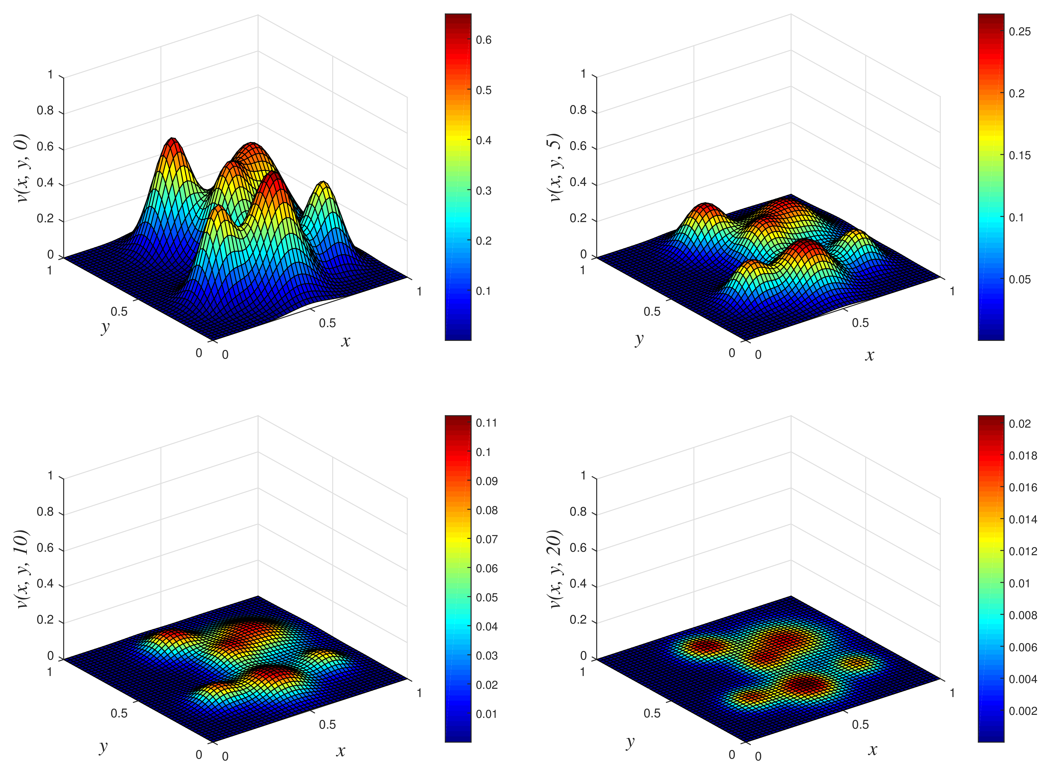
• Results of Numerical Experiment 2
  All the three methods give almost the same profile at times $5,10$ and 20. One observation from these numerical simulations is that the biofilm colonies are annihilated as we progress in time, and this is due to rate of reaction being negative (in this case, $r=-0.17$). We obtained the plot of the numerical solution using NSFD1 vs. x vs. y in Figure 5. We have omitted graphical results using the two other methods (EPSS and Classical schemes) due to similar results and the limitation of the number of pages for this manuscript. The profiles obtained are similar to those reported by Maciaz-Diaz et al. [8].

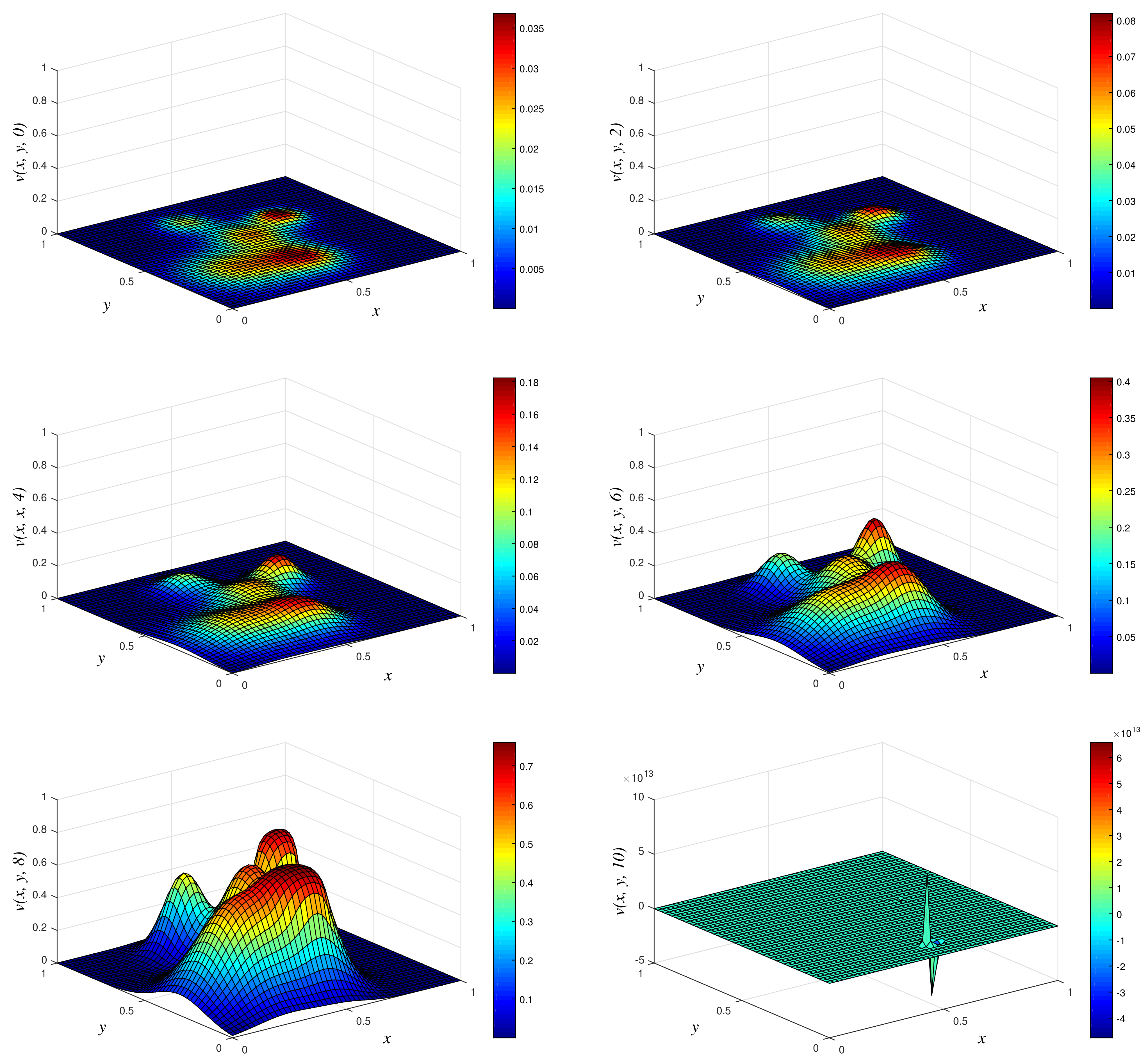
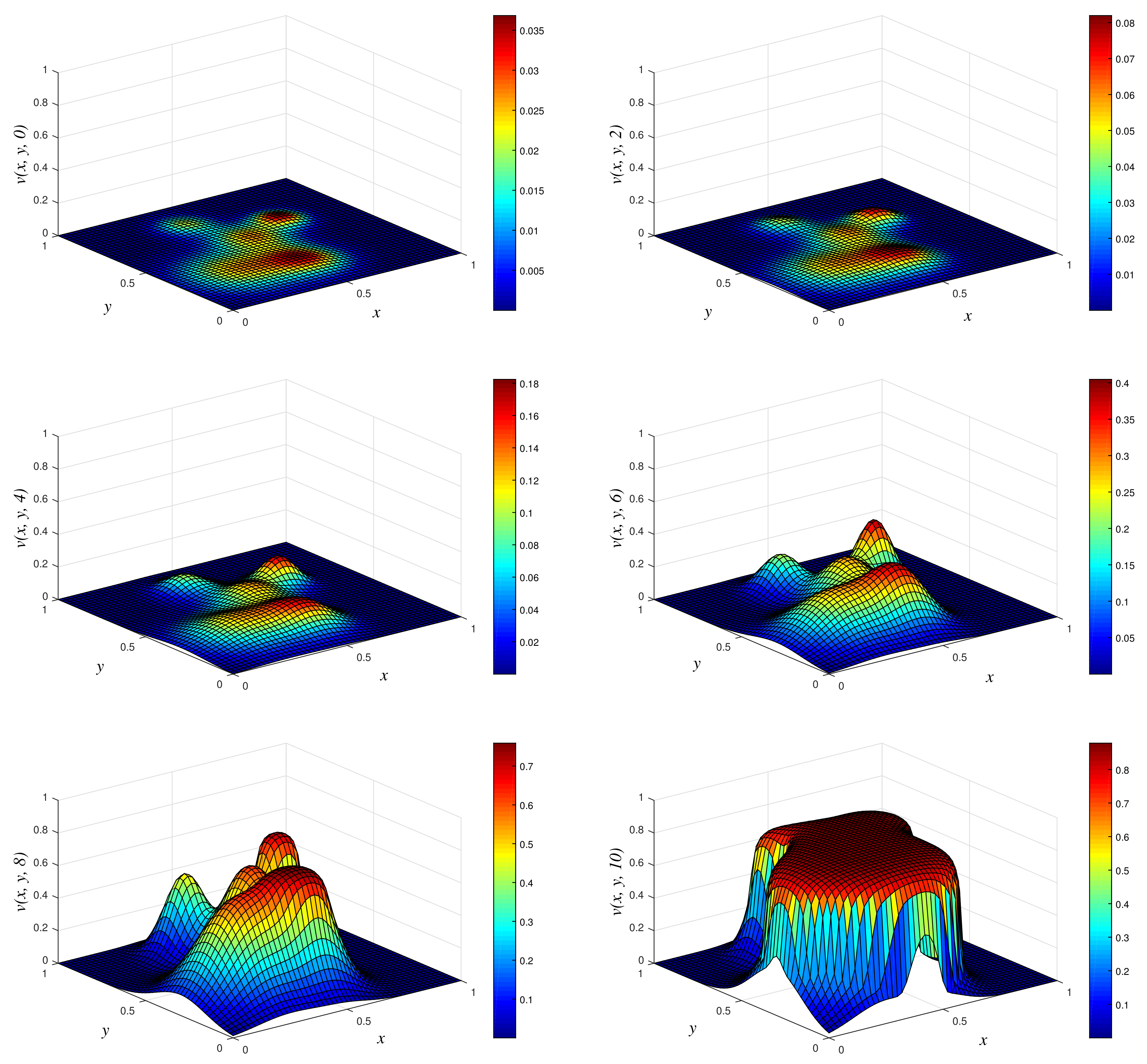
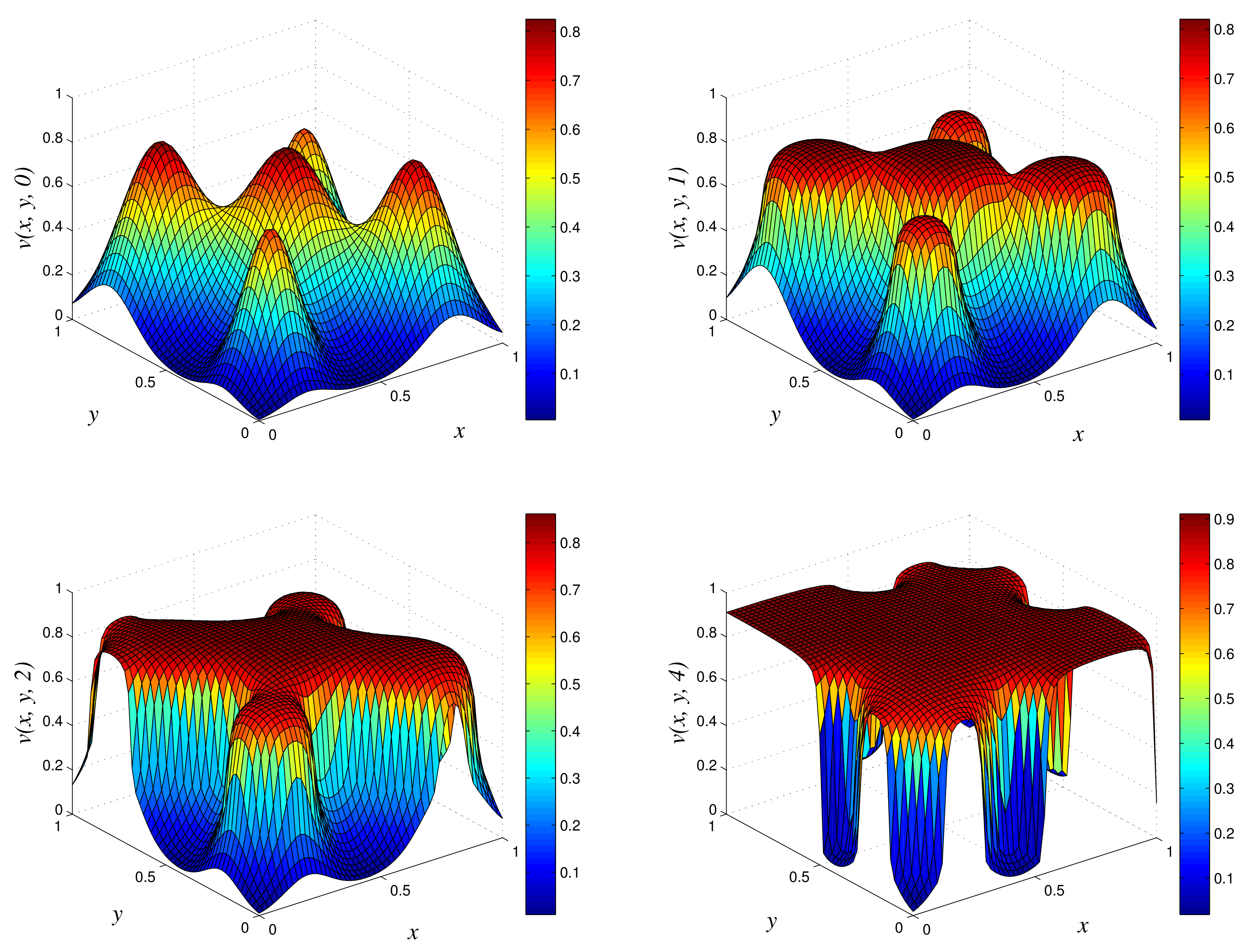
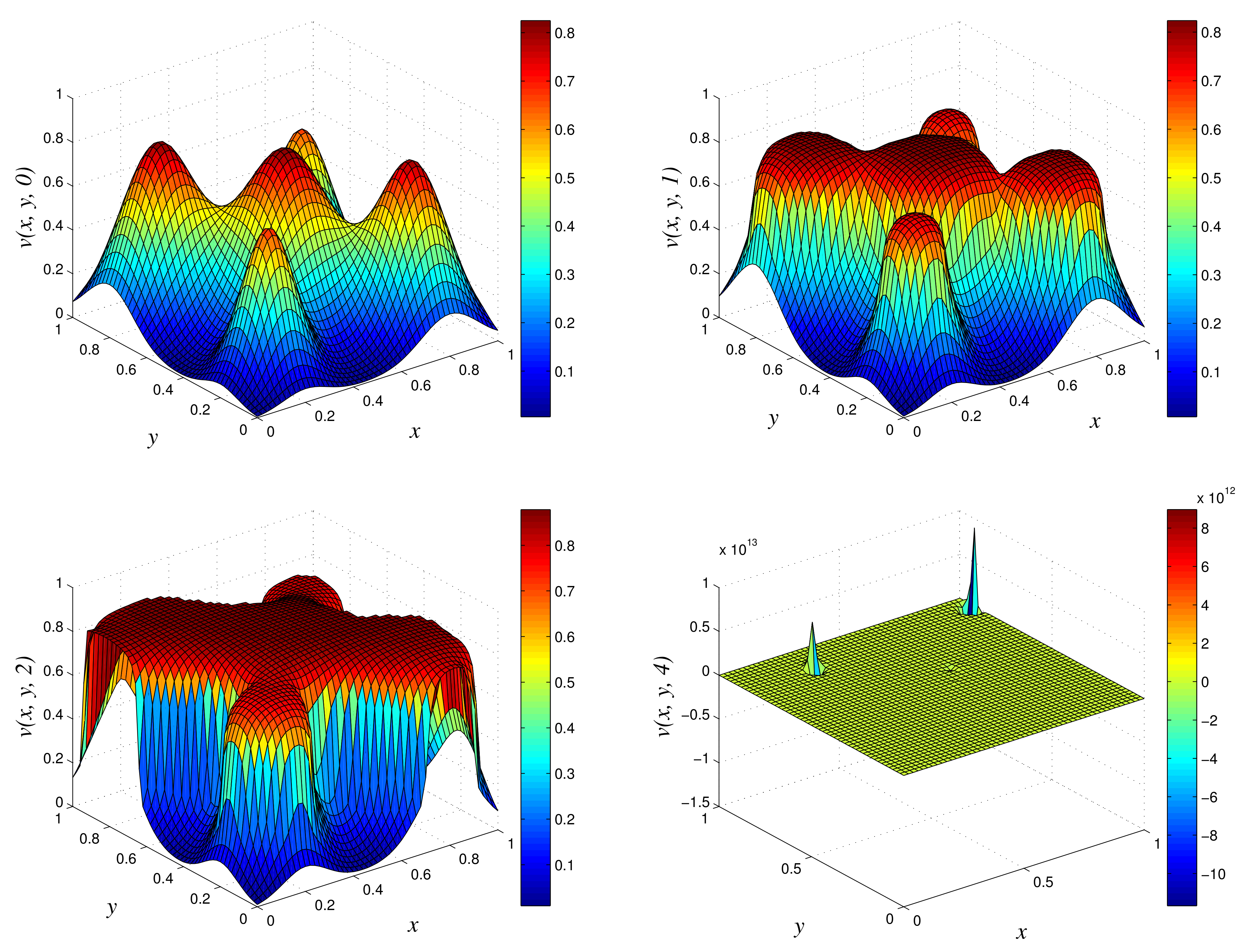
• Results of Numerical Experiment 3
  Experiment 3 is a typical example in which the biofilm builds up with time. We display the results of the numerical solution vs. x vs. y using NSFD1 and classical schemes in Figure 6 and Figure 7. We obtained similar results with all the three methods at times $t=1$ and 2. However, at $t=4$, we observe a blow up when the classical scheme is used, and we still find a positive definite and bounded solution at $t=4$ when we use NSFD1. The results from the NSFD1 scheme presented here agree with those from the EPPS scheme.

• Results of experiment 1

Figure 2. 3D plots of numerical solution vs. x vs. y using NSFD1 scheme at times $t=0,2,4,6,8$ and 10. We used spatial step sizes $h_x=h_y=0.02$ and time step $k=0.0004$.

Figure 2. 3D plots of numerical solution vs. x vs. y using NSFD1 scheme at times $t=0,2,4,6,8$ and 10. We used spatial step sizes $h_x=h_y=0.02$ and time step $k=0.0004$.

Figure 3. 3D plots of numerical solution vs. x vs. y using classical scheme at times $t=0,2,4,6,8$ and 10. We used spatial step sizes $h_x=h_y=0.02$ and time step $k=0.0004$.

Figure 3. 3D plots of numerical solution vs. x vs. y using classical scheme at times $t=0,2,4,6,8$ and 10. We used spatial step sizes $h_x=h_y=0.02$ and time step $k=0.0004$.

Figure 4. 3D plots of numerical solution vs. x vs. y using EPSS scheme at times $t=0,2,4,6,8$ and 10. We used spatial step sizes $h_x=h_y=0.02$ and time step $k=0.0004$.

Figure 4. 3D plots of numerical solution vs. x vs. y using EPSS scheme at times $t=0,2,4,6,8$ and 10. We used spatial step sizes $h_x=h_y=0.02$ and time step $k=0.0004$.

• Results of experiment 2

Figure 5. 3D plots of numerical solution vs. x vs. y using NSFD1 scheme at times $t=0,5,10$ and 20. We used spatial step sizes $h_x=h_y=0.02$ and time step $k=0.01$.

Figure 5. 3D plots of numerical solution vs. x vs. y using NSFD1 scheme at times $t=0,5,10$ and 20. We used spatial step sizes $h_x=h_y=0.02$ and time step $k=0.01$.

• Results of experiment 3

Figure 6. 3D plots of numerical solution vs. x vs. y using NSFD1 scheme at times $t=0,1,2$ and 4. We used spatial step sizes $h_x=h_y=0.02$ and time step $k=0.0001$.

Figure 6. 3D plots of numerical solution vs. x vs. y using NSFD1 scheme at times $t=0,1,2$ and 4. We used spatial step sizes $h_x=h_y=0.02$ and time step $k=0.0001$.

Figure 7. 3D plots of numerical solution vs. x vs. y using classical scheme at times $t=0,1,2$ and 4. We used spatial step sizes $h_x=h_y=0.02$ and time step $k=0.0001$.

Figure 7. 3D plots of numerical solution vs. x vs. y using classical scheme at times $t=0,1,2$ and 4. We used spatial step sizes $h_x=h_y=0.02$ and time step $k=0.0001$.

7. Coupled Substrate–Biomass System

The coupled substrate and biomass system of equations is given by

$$\begin{array}{c}\hfill {\displaystyle \frac{\partial u}{\partial t}}={\Gamma }_1\left({\displaystyle \frac{{\partial }^{2}u}{\partial x^2}}+{\displaystyle \frac{{\partial }^{2}u}{\partial y^2}}\right)-{\Gamma }_3{\displaystyle \frac{uv}{{\Gamma }_4+u}}\mathrm{and}\\ \hfill {\displaystyle \frac{\partial v}{\partial t}}={\Gamma }_{2}D\left(v\right)\left({\displaystyle \frac{{\partial }^{2}v}{\partial x^2}}+{\displaystyle \frac{{\partial }^{2}v}{\partial y^2}}\right)+{\Gamma }_2{D}^{\prime }\left(v\right)\left({\left({\displaystyle \frac{\partial v}{\partial x}}\right)}^2+{\left({\displaystyle \frac{\partial v}{\partial y}}\right)}^2\right)-rv+{\Gamma }_5{\displaystyle \frac{uv}{{\Gamma }_4+u}},\end{array}$$

(33)

with initial and boundary conditions

$$\left\{\begin{array}{c}u(\mathbf{x},t)=1,v(\mathbf{x},t)=0,\forall \mathbf{x}\in \partial \mathsf{\Omega },t\ge 0,\hfill \\ u(\mathbf{x},t)=u_0\left(\mathbf{x}\right),v(\mathbf{x},t)=v_0\left(\mathbf{x}\right).\hfill \end{array}\right.$$

(34)

where we define $D\left(v\right)={\displaystyle \frac{v^{\lambda }}{{(1-v)}^{\mu }}}$.

We begin by showing the discretization of each term comprising Equation (33)

$${\displaystyle \frac{\partial u}{\partial t}}\approx {\displaystyle \frac{u_{i,j}^{n+1}-u_{i,j}^n}{k}}\mathrm{and}{\displaystyle \frac{\partial v}{\partial t}}\approx {\displaystyle \frac{v_{i,j}^{n+1}-v_{i,j}^n}{k}}.$$

(35)

We use the following approximations:

$${\displaystyle \frac{{\partial }^{2}u}{\partial x^2}}\approx {\displaystyle \frac{u_{i+1,j}^n-2u_{i,j}^{n+1}+u_{i-1,j}^n}{{\left(h_x\right)}^2}}\mathrm{and}{\displaystyle \frac{{\partial }^{2}u}{\partial y^2}}\approx {\displaystyle \frac{u_{i,j+1}^n-2u_{i,j}^{n+1}+u_{i,j-1}^n}{{\left(h_y\right)}^2}}.$$

(36)

The Michaelis–Menten form of the reaction in the substrate concentration equation is discretized using classical and non-classical approximations as

$${\Gamma }_3{\displaystyle \frac{uv}{{\Gamma }_4+u}}\approx {\Gamma }_3{\displaystyle \frac{u_{i,j}^{n+1}{v}_{i,j}^n}{{\Gamma }_4+u_{i,j}^n}}.$$

(37)

The substrate concentration in a discretized form thus becomes

$${\displaystyle \frac{u_{i,j}^{n+1}-u_{i,j}^n}{\varphi \left(k\right)}}={\Gamma }_1\left({\displaystyle \frac{u_{i+1,j}^n-2u_{i,j}^{n+1}+u_{i-1,j}^n}{{\left(h_x\right)}^2}}+{\displaystyle \frac{u_{i,j+1}^n-2u_{i,j}^{n+1}+u_{i,j-1}^n}{{\left(h_y\right)}^2}}\right)-{\Gamma }_3{\displaystyle \frac{u_{i,j}^{n+1}{v}_{i,j}^n}{{\Gamma }_4+u_{i,j}^n}}$$

(38)

After some mathematical manipulation, we have

$$u_{i,j}^{n+1}={\displaystyle \frac{u_{i,j}^n+R{\Gamma }_1(u_{i+1,j}^n+u_{i-1,j}^n)+R{\Gamma }_1(u_{i,j+1}^n+u_{i,j-1}^n)}{1+4{\Gamma }_{1}R+k{\Gamma }_3{\displaystyle \frac{v_{i,j}^n}{{\Gamma }_4+u_{i,j}^n}}}}.$$

(39)

We use the earlier approximation of Equations (12), (13) and (16) for the biomass quantity v. The reactions take the form

$$rv\approx r{v}_{i,j}^{n+1}\mathrm{and}{\Gamma }_5{\displaystyle \frac{uv}{{\Gamma }_4+u}}\approx {\Gamma }_5{\displaystyle \frac{u_{i,j}^n{v}_{i,j}^n}{{\Gamma }_4+u_{i,j}^n}}.$$

(40)

In a concise form, we obtain

$$\begin{array}{c}\hfill v_{i,j}^{n+1}={\displaystyle \frac{0.25{\Gamma }_{2}R\left(D\left(v_{i+1,j}^n\right)\left(3v_{i+1,j}^n+v_{i-1,j}^n\right)+\left(v_{i-1,j}^n\right)\left(v_{i+1,j}^n+3v_{i-1,j}^n\right)\right)+v_{i,j}^n+k{\Gamma }_5{\displaystyle \frac{u_{i,j}^n{v}_{i,j}^n}{{\Gamma }_4+u_{i,j}^n}}}{1+{\Gamma }_{2}R\left(D\left(v_{i-1,j}^n\right)+D\left(v_{i+1,j}^n\right)\right)+{\Gamma }_{2}R\left(D\left(v_{i,j-1}^n\right)+D\left(v_{i,j+1}^n\right)\right)+kr}}\\ \hfill +{\displaystyle \frac{0.25{\Gamma }_{2}R\left(D\left(v_{i,j+1}^n\right)\left(3v_{i,j+1}^n+v_{i,j-1}^n\right)+D\left(v_{i,j-1}^n\right)\left(v_{i,j+1}^n+3v_{i,j-1}^n\right)\right)}{1+{\Gamma }_{2}R\left(D\left(v_{i-1,j}^n\right)+D\left(v_{i+1,j}^n\right)\right)+{\Gamma }_{2}R\left(D\left(v_{i,j-1}^n\right)+D\left(v_{i,j+1}^n\right)\right)+kr}}.\end{array}$$

(41)

The coupled nutritive substrate–biomass discretization (NSFD2) is

$$\left\{\begin{array}{c}{u}_{i,j}^{n+1}={\displaystyle \frac{u_{i,j}^n+R{\Gamma }_1(u_{i+1,j}^n+u_{i-1,j}^n)+R{\Gamma }_1(u_{i,j+1}^n+u_{i,j-1}^n)}{1+4{\Gamma }_{1}R+k{\Gamma }_3{\displaystyle \frac{v_{i,j}^n}{{\Gamma }_4+u_{i,j}^n}}}}.\hfill \\ v_{i,j}^{n+1}={\displaystyle \frac{0.25{\Gamma }_{2}R\left(D\left(v_{i+1,j}^n\right)\left(3v_{i+1,j}^n+v_{i-1,j}^n\right)+D\left(v_{i-1,j}^n\right)\left(v_{i+1,j}^n+3v_{i-1,j}^n\right)\right)+v_{i,j}^n}{1+{\Gamma }_{2}R\left(D\left(v_{i-1,j}^n\right)+D\left(v_{i+1,j}^n\right)\right)+{\Gamma }_{2}R\left(D\left(v_{i,j-1}^n\right)+D\left(v_{i,j+1}^n\right)\right)+kr}}\hfill \\ \hfill \hspace{1em} +{\displaystyle \frac{k{\Gamma }_5{\displaystyle \frac{u_{i,j}^n{v}_{i,j}^n}{{\Gamma }_4+u_{i,j}^n}}+0.25{\Gamma }_{2}R\left(D\left(v_{i,j+1}^n\right)\left(3v_{i,j+1}^n+v_{i,j-1}^n\right)+D\left(v_{i,j-1}^n\right)\left(v_{i,j+1}^n+3v_{i,j-1}^n\right)\right)}{1+{\Gamma }_{2}R\left(D\left(v_{i-1,j}^n\right)+D\left(v_{i+1,j}^n\right)\right)+{\Gamma }_{2}R\left(D\left(v_{i,j-1}^n\right)+D\left(v_{i,j+1}^n\right)\right)+kr}}.\end{array}\right.$$

(42)

Suitable discrete boundary (homogeneous Dirichlet or Neumann) conditions on the edges are imposed. The conditions take the forms

$$\left\{\begin{array}{c}{u}_{1,j}^n={\left(u_{2,j}^n\right)}^{\alpha }{u}_{M+1,j}^n={\left(u_{M,j}^n\right)}^{\beta },1\le j\le M+1,\hfill \\ u_{i,1}^n={\left(u_{i,2}^n\right)}^{\gamma }{u}_{i,N+1}^n={\left(u_{i,N}^n\right)}^{\zeta },1\le i\le N+1,\hfill \\ v_{1,j}^n=\alpha v_{2,j}^n,v_{M+1,j}^n=\beta v_{M,j}^n,1\le j\le M+1,\hfill \\ v_{i,1}^n=\gamma v_{i,2}^n,v_{i,N+1}^n=\zeta v_{i,N}^n,1\le i\le N+1.\hfill \end{array}\right.$$

(43)

The homogeneous Neumann boundary condition is enforced if the constants $\alpha =\beta =\gamma =\zeta =1$; otherwise, the homogeneous Dirichlet is used when $\alpha =\beta =\gamma =\zeta =0$. We now seek to show the conservation of physical properties by the schemes in Equation (42).

Remark 4

(Positivity). The schemes from Equation (42) are strictly positive since all the terms in the numerator and denominator contain positive terms only.

• Boundedness

We show that, for the numerical scheme of Equation (42),

$$0<u_{i,j}^n<1\Rightarrow 0<u_{i,j}^{n+1}<1\mathrm{and}0<v_{i,j}^n<1\Rightarrow 0<v_{i,j}^{n+1}<1.$$

for all i and j.

Proof. 

Since $u_{i,j}^n<1$, then $max\{u_{i+1,j}^n,u_{i-1,j}^n,u_{i,j+1}^n,u_{i,j-1}^n\}<1$ and $0<v_{i,j}^n<1$. Hence,

$$\begin{array}{l}{u}_{i,j}^{n+1}={\displaystyle \frac{u_{i,j}^n+R{\Gamma }_1(u_{i+1,j}^n+u_{i-1,j}^n)+R{\Gamma }_1(u_{i,j+1}^n+u_{i,j-1}^n)}{1+4{\Gamma }_{1}R+k{\Gamma }_3{\displaystyle \frac{v_{i,j}^n}{{\Gamma }_4+u_{i,j}^n}}}}\\ \hspace{1em}\hspace{1em}\le {\displaystyle \frac{1+4R{\Gamma }_1}{1+4{\Gamma }_{1}R+k{\Gamma }_3{\displaystyle \frac{v_{i,j}^n}{{\Gamma }_4+u_{i,j}^n}}}},\\ \hspace{1em}\hspace{1em}\le 1.\end{array}$$

(44)

Since $k{\Gamma }_3{\displaystyle \frac{v_{i,j}^n}{{\Gamma }_4+u_{i,j}^n}}>0$ for the non-negative initial condition $v_{i,j}^n$. For $v_{i,j}^{n+1}$, we consider the boundedness condition of the NSFD1 scheme. □

Proposition 2.

[Boundedness of the scheme]

• If $k\left({\Gamma }_5{\displaystyle \frac{u_{i,j}^n{v}_{i,j}^n}{{\Gamma }_4+u_{i,j}^n}}-r\right)<\xi \eta$, any random time-step k will always ensure $v_{i,j}^{n+1}<1$ whenever $v_{i,j}^n\in [0,1]$ and $u_{i,j}^n\in [0,1]$.
• If $k\left({\Gamma }_5{\displaystyle \frac{u_{i,j}^n{v}_{i,j}^n}{{\Gamma }_4+u_{i,j}^n}}-r\right)>\xi \eta$ and $k\le {\displaystyle \frac{1-v_{i,j}^n}{\left(r-{\Gamma }_5{\displaystyle \frac{u_{i,j}^n{v}_{i,j}^n}{{\Gamma }_4+u_{i,j}^n}}\right)-\xi \eta }}$ hold, then the numerical solution satisfies $v_{i,j}^{n+1}<1$ whenever $v_{i,j}^n<1$.

The proof follows the same procedure as in NSFD1. In order to ascertain the effectiveness of our scheme for Equation (33), we implemented the classical scheme given as

$${\displaystyle \frac{u_{i,j}^{n+1}-u_{i,j}^n}{k}}={\Gamma }_1\left({\displaystyle \frac{u_{i+1,j}^n-2u_{i,j}^n+u_{i-1,j}^n}{{\left(h_x\right)}^2}}+{\displaystyle \frac{u_{i,j+1}^n-2u_{i,j}^n+u_{i,j-1}^n}{{\left(h_y\right)}^2}}\right)-{\Gamma }_3{\displaystyle \frac{u_{i,j}^n{v}_{i,j}^n}{{\Gamma }_4+u_{i,j}^n}},$$

(45)

$$\begin{array}{c}\hfill {\displaystyle \frac{v_{i,j}^{n+1}-v_{i,j}^n}{k}}={\Gamma }_2{\displaystyle \frac{D\left(v_{i+1,j}^n\right)-D\left(v_{i,j}^n\right)}{v_{i+1,j}^n-v_{i,j}^n}}{\left({\displaystyle \frac{v_{i+1,j}^n-v_{i,j}^n}{h_x}}\right)}^2+{\Gamma }_2{\displaystyle \frac{D\left(v_{i,j+1}^n\right)-D\left(v_{i,j}^n\right)}{v_{i,j+1}^n-v_{i,j}^n}}{\left({\displaystyle \frac{v_{i,j+1}^n-v_{i,j}^n}{h_y}}\right)}^2+\\ \hfill {\Gamma }_{2}D\left(v_{i,j}^n\right)\left({\displaystyle \frac{v_{i+1,j}^n-2v_{i,j}^n+v_{i-1,j}^n}{{\left(h_x\right)}^2}}+{\displaystyle \frac{v_{i,j+1}^n-2v_{i,j}^n+v_{i,j-1}^n}{{\left(h_y\right)}^2}}\right)-r{v}_{i,j}^n+{\Gamma }_5{\displaystyle \frac{u_{i,j}^n{v}_{i,j}^n}{{\Gamma }_4+u_{i,j}^n}}.\end{array}$$

(46)

The classical scheme in compact form takes the form

$$\left\{\begin{array}{l}{u}_{i,j}^{n+1}=u_{i,j}^n+R{\Gamma }_1(u_{i+1,j}^n-2u_{i,j}^n+u_{i-1,j}^n)+R{\Gamma }_1(u_{i,j+1}^n-2u_{i,j}^n+u_{i,j-1}^n)-k{\Gamma }_3{\displaystyle \frac{u_{i,j}^n{v}_{i,j}^n}{{\Gamma }_4+u_{i,j}^n}}.\\ v_{i,j}^{n+1}={\Gamma }_{2}R\left(D\left(v_{i+1,j}^n\right)-D\left(v_{i,j}^n\right)\right)\left(v_{i+1,j}^n-v_{i,j}^n\right)+{\Gamma }_{2}R\left(D\left(v_{i,j+1}^n\right)-D\left(v_{i,j}^n\right)\right)\left(v_{i,j+1}^n-v_{i,j-1}^n\right)+\\ (1-kr)v_{i,j}^n+R{\Gamma }_{2}D\left(v_{i,j}^n\right)(v_{i+1,j}^n-2v_{i,j}^n+v_{i-1,j}^n)+R{\Gamma }_{2}D\left(v_{i,j}^n\right)(v_{i,j+1}^n-2v_{i,j}^n+v_{i,j-1}^n)+k{\Gamma }_5{\displaystyle \frac{u_{i,j}^n{v}_{i,j}^n}{{\Gamma }_4+u_{i,j}^n}}.\end{array}\right.$$

(47)

8. Numerical Results of Problem 2

We present two numerical simulations for the coupled substrate–biomass equations to examine the accuracy and effectiveness of our proposed scheme (NSFD2).

Experiment 4.

Let $\mathsf{\Omega }\subset {\mathbb{R}}^2$, which is defined as $\mathsf{\Omega }=\left[\right(0,1)\times (0,1\left)\right]$. We consider an initial profile with constant and Gaussian functions of the form

$$u(x,y,0)=1andv(x,y,0)=\sum _{p=1}^5{C}_p{e}^{-w_p\left|\right|\mathit{X}-{\mathit{X}}_p{\left|\right|}^2},forall\mathit{X}\in \mathsf{\Omega },$$

(48)

for u and v, respectively, where $C_1=0.68,C_2=0.65,C_3=0.80,C_4=0.78$, $C_5=0.70$, $w_1=60,w_2=50$, $w_3=30$, $w_4=35,w_5=20$, ${\mathit{X}}_1=(0.20,0.20)$, ${\mathit{X}}_2=(0.60,0.20)$, ${\mathit{X}}_3=(0.50,0.50)$, ${\mathit{X}}_4=(0.30,0.80)$, ${\mathit{X}}_5=(0.80,0.80)$. We set $\lambda =4.0$, $\mu =4.0$, ${\Gamma }_1=0.0015$, ${\Gamma }_2=0.01$, ${\Gamma }_3=0.65$, ${\Gamma }_4=0.40$, ${\Gamma }_5=0.08$ and $r=0.40$. The homogeneous Dirichlet conditions are considered on the boundary point of $\mathsf{\Omega }$.

Experiment 5.

Let $\mathsf{\Omega }\subset {\mathbb{R}}^2$ be defined as $\mathsf{\Omega }=\left\{\right(0,1)\times (0,1\left)\right\}$. We consider an initial profile of the form

$$u(x,y,0)=1andv(x,y,0)=\sum _{p=1}^5{C}_p{e}^{-w_p\left|\right|\mathit{X}-{\mathit{X}}_p{\left|\right|}^2},forall\mathit{X}\in \mathsf{\Omega }.$$

(49)

Where $C_1=0.47,C_2=0.50$, $C_3=0.60$, $C_4=0.50,C_5=0.60$, $w_1=200,w_2=50$, $w_3=280,w_4=50$, $w_5=280$, ${\mathit{X}}_1=(0.20,0.20)$, ${\mathit{X}}_2=(0.60,0.20)$, ${\mathit{X}}_3=(0.50,0.50)$, ${\mathit{X}}_4=(0.30,0.80)$, ${\mathit{X}}_5=(0.80,0.80)$. We set $\lambda =4.0$, $\mu =4.0$, ${\Gamma }_1=0.0015$, ${\Gamma }_2=0.0001$, ${\Gamma }_3=0.65$, ${\Gamma }_4=0.40$, ${\Gamma }_5=0.60$ and $r=0.06$. The homogeneous Dirichlet conditions are considered on the boundary point of $\mathsf{\Omega }$.

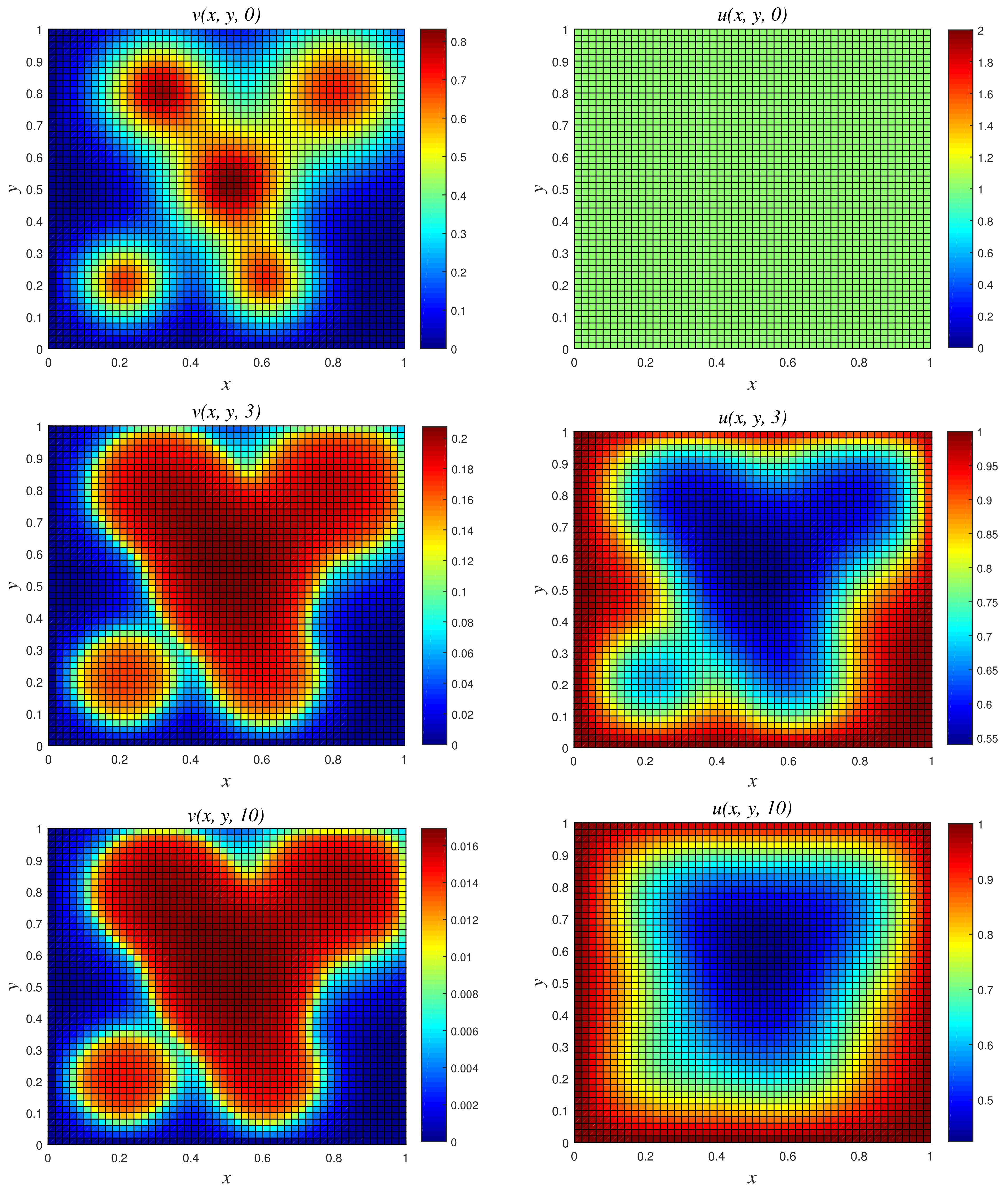
• Results of Numerical Experiment 4
  Experiment 4 is a classic example where the biomass density decreases with time while the nutritive substrate increases within the bounded region. This is due to the fact that the biomass decay rate r exceeds the maximum specific growth rate ${\Gamma }_5$. The classical scheme does not maintain good physical properties of the coupled PDEs for this attenuation system, as depicted in Figure 8, where a blow up occurs at time $t=3$ and 10. On the other hand, NSFD2 maintains dynamical consistency, and realistic results are displayed using the scheme in Figure 9.

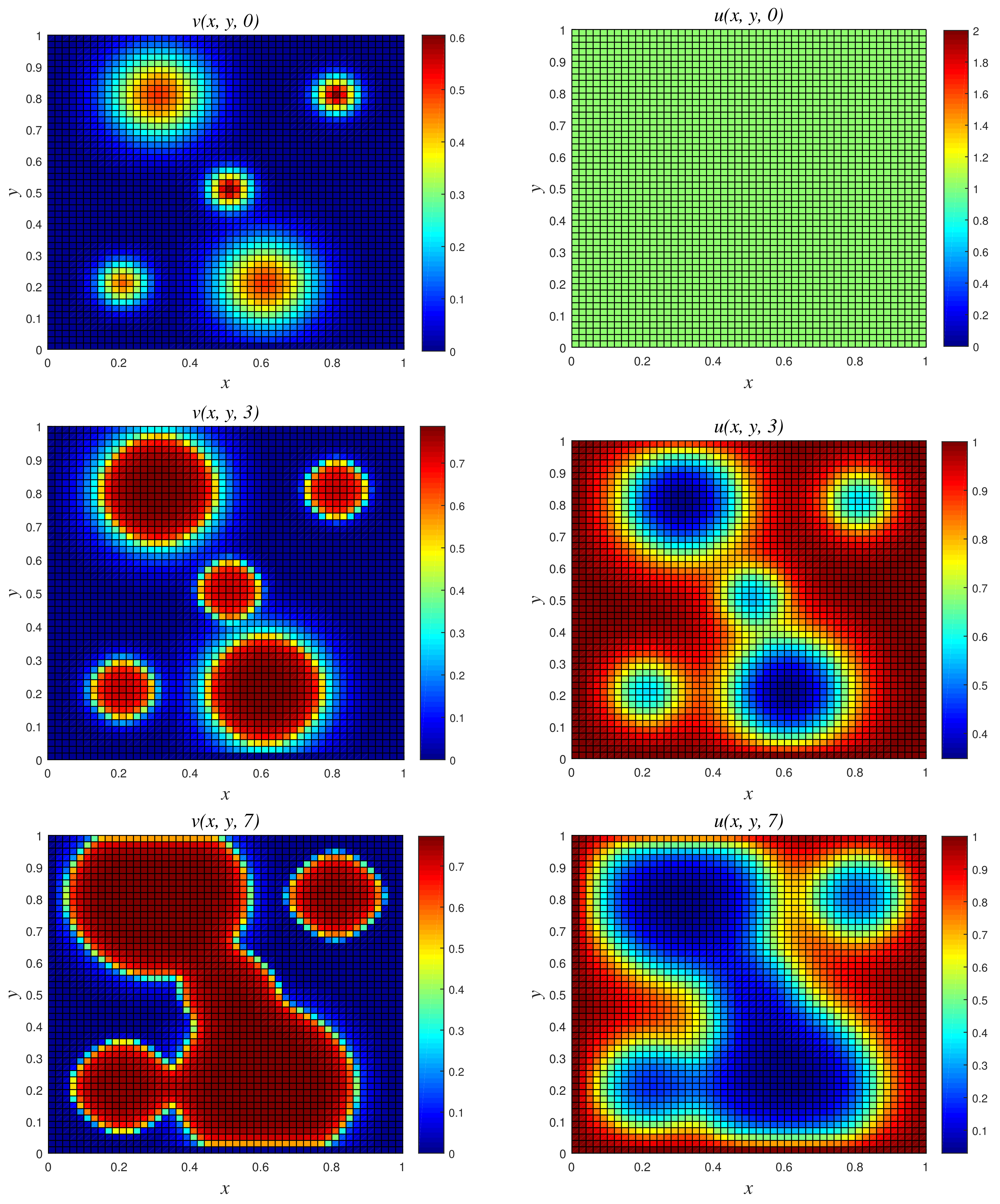
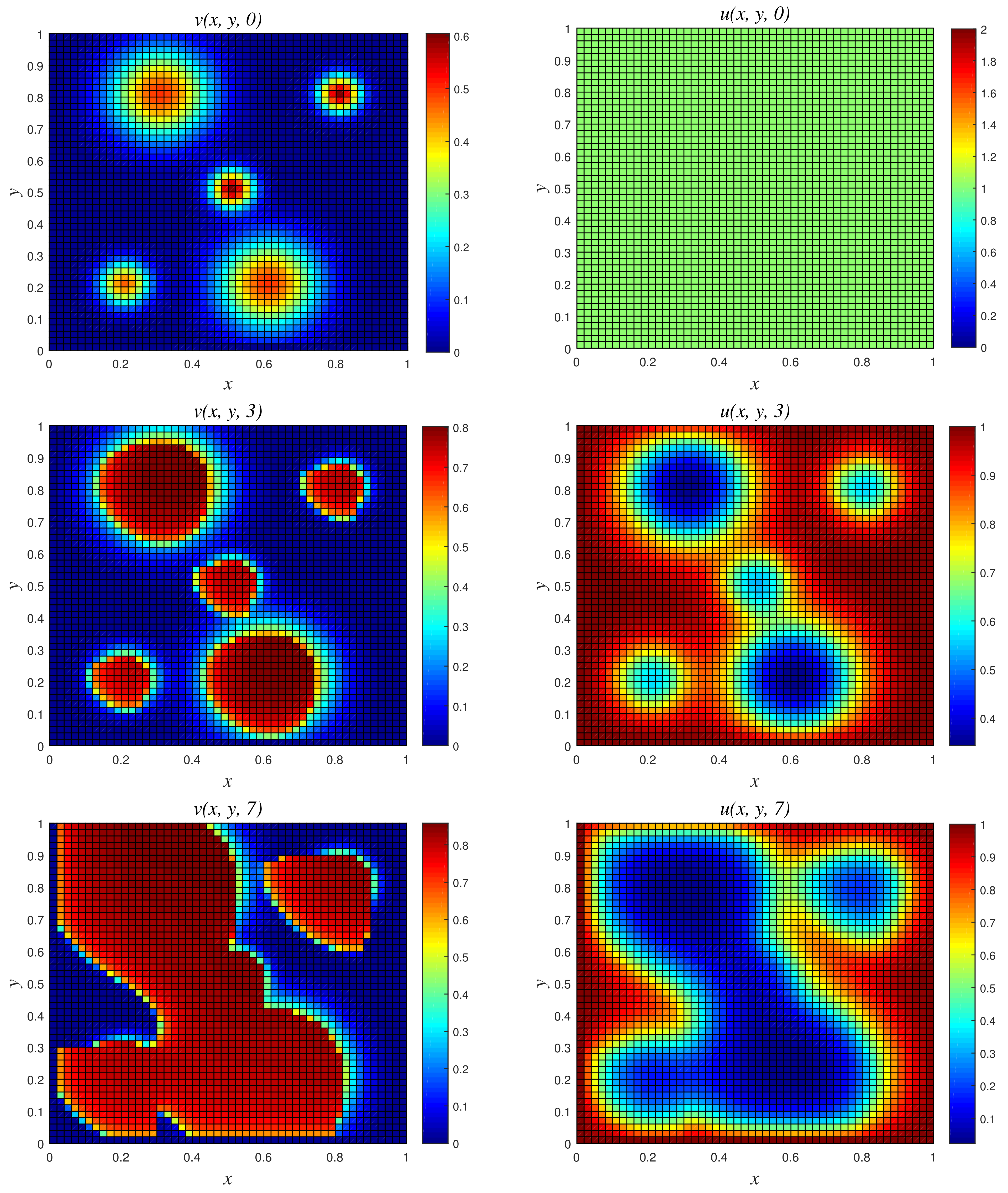
• Results of Numerical Experiment 5
  The biofilm density appears to be increasing and spreading with the passage of time. This is due to the fact that the biomass degradation constant r is substantially lower than the maximal specific growth rate ${\Gamma }_5.$ NSFD2 and classical schemes are efficient and both give bounded solutions; see Figure 10 and Figure 11. However, we observe that the result of the classical scheme does not look stable when compared to the NSFD2 scheme.

• Results of experiment 4

Figure 8. 3D plots of numerical solution vs. x vs. y using classical scheme at times $t=0,3$ and 10. We used spatial step sizes $h_x=h_y=0.02$ and time step $k=0.0004$.

Figure 8. 3D plots of numerical solution vs. x vs. y using classical scheme at times $t=0,3$ and 10. We used spatial step sizes $h_x=h_y=0.02$ and time step $k=0.0004$.

Figure 9. 3D plots of numerical solution vs. x vs. y using NSFD2 scheme at times $t=0,3$ and 10. We used spatial step sizes $h_x=h_y=0.02$ and time step $k=0.0004$.

Figure 9. 3D plots of numerical solution vs. x vs. y using NSFD2 scheme at times $t=0,3$ and 10. We used spatial step sizes $h_x=h_y=0.02$ and time step $k=0.0004$.

• Results of experiment 5

Figure 10. 3D plots of numerical solution vs. x vs. y using NSFD2 scheme at times $t=0,3$ and 7. We used spatial step sizes $h_x=h_y=0.02$ and time step $k=0.0004$.

Figure 10. 3D plots of numerical solution vs. x vs. y using NSFD2 scheme at times $t=0,3$ and 7. We used spatial step sizes $h_x=h_y=0.02$ and time step $k=0.0004$.

Figure 11. 3D plots of numerical solution vs. x vs. y using classical scheme at times $t=0,3$ and 7. We used spatial step sizes $h_x=h_y=0.02$ and time step $k=0.0004$.

Figure 11. 3D plots of numerical solution vs. x vs. y using classical scheme at times $t=0,3$ and 7. We used spatial step sizes $h_x=h_y=0.02$ and time step $k=0.0004$.

9. Conclusions

In this paper, the study of biofilm formation and the coupled substrate–biofilm relation using some finite difference schemes was investigated. These real-time scenarios were modelled mathematically using one parabolic PDE and a system of two parabolic PDEs in Equations (6) and (33), respectively. The use of the finite difference scheme is due to the difficulty in obtaining an analytical solution, although the existence and uniqueness of the solution have been established for the equations. To this end, we designed an efficient non-standard finite difference scheme (NSFD1) for the biofilm formation which preserves the conservative properties such as positivity and boundedness. We have efficiently handled the non-linear diffusion term by introducing a new linearizing operator. The excellent performance of our proposed scheme (NSFD1) motivated us to construct a novel structure-preserving scheme (NSFD2) for the coupled substrate–biofilm equation. NSFD2 showed good behaviour with conservation of physical properties. The proposed scheme demonstrates that the biofilm generation and nutritive substrate development processes are significantly interconnected. Our proposed schemes competes favourably well with earlier known results in the literature; see

Table 1. Rate of convergence in time using experiment 1 for NSFD1 and classical schemes for $h=0.02$ at time $t=8$.

k	NSFD1 (19)		Classical (25)
	${\mathit{E}}_{\mathit{k}}$	${\mathit{R}}^{\mathit{T}}$	${\mathit{E}}_{\mathit{k}}$	${\mathit{R}}^{\mathit{T}}$
0.0032	$1.0149\times {10}^{-2}$	–	$2.6820\times {10}^{-3}$	–
0.0016	$5.8124\times {10}^{-3}$	0.8041	$1.3602\times {10}^{-3}$	0.9794
0.0008	$3.1437\times {10}^{-3}$	0.8867	$6.8479\times {10}^{-4}$	$0.9900$
0.0004	$1.6404\times {10}^{-3}$	0.9384	$3.4355\times {10}^{-4}$	$0.9951$
0.0002	$8.3880\times {10}^{-4}$	0.9676	$1.7206\times {10}^{-4}$	0.9976

,

Table 2. Rate of convergence in time using experiment 2 for NSFD1 and classical schemes for $h=0.02$ at time $t=5$.

k	NSFD1 (19)		Classical (25)
	${\mathit{E}}_{\mathit{k}}$	${\mathit{R}}^{\mathit{T}}$	${\mathit{E}}_{\mathit{k}}$	${\mathit{R}}^{\mathit{T}}$
0.02	$1.8664\times {10}^{-3}$	–	$5.0464\times {10}^{-4}$	–
0.01	$9.1021\times {10}^{-4}$	1.0359	$2.5146\times {10}^{-4}$	1.0049
0.005	$4.4931\times {10}^{-4}$	1.0184	$1.2551\times {10}^{-4}$	1.0025
0.0025	$2.2400\times {10}^{-4}$	1.0042	$6.2706\times {10}^{-5}$	1.0011

,

Table 3. Rate of convergence in time using experiment 3 for NSFD1 and classical schemes for $h=0.02$ at time $t=1$.

k	NSFD1 (19)		Classical (25)
	${\mathit{E}}_{\mathit{k}}$	${\mathit{R}}^{\mathit{T}}$	${\mathit{E}}_{\mathit{k}}$	${\mathit{R}}^{\mathit{T}}$
0.0016	$1.1687\times {10}^{-2}$	–	$1.0057\times {10}^{-3}$	–
0.0008	$7.9887\times {10}^{-3}$	0.5488	$9.9989\times {10}^{-4}$	$0.00848$
0.0004	$4.7608\times {10}^{-3}$	0.7467	$5.0162\times {10}^{-4}$	$0.9951$
0.0002	$2.6166\times {10}^{-3}$	0.8635	$2.5121\times {10}^{-4}$	$0.9977$
0.0001	$1.3744\times {10}^{-3}$	0.9288	$1.2570\times {10}^{-4}$	0.9989

and

Table 4. Comparison of some finite-difference methods used for the mathematical modelling of biofilm formation to simulate Equation (6).

Properties	NSFD1 (19)	Classical (25)	EPPS (29)	Maciaz-Diaz et al. [8]
Positivity	Positive	Not Positive	Positive	Positive
Boundedness	Bounded	Not Bounded	Bounded	Bounded
Class of Scheme	Explicit	Explicit	Explicit	Explicit
Implementation	Linear	Linear	Linear	Non-linear
Construction	Easy	Easy	Moderate	Moderate

. In regards to the classical scheme, a blow up occurred at time $t=10,4$ and 3 for experiments 1, 3 and 4, respectively. In addition, it is extremely difficult to obtain a stability region, especially when dealing with coupled systems of PDEs. The technique in this study can be applied to other areas of mathematical biology and sciences. The results here elaborate the benefits of the non-standard approximations over the classical approximations in practical applications. In our future study, a structural finite difference scheme will be proposed to handle the modified mathematical model to Equation (33) as well as a dynamically consistent finite difference scheme for the system of advection–diffusion–reaction equations arising in quorum sensing. In addition, we will investigate the effects of random noise when incorporated into the equations.

References

- Perez-Velazquez, J.; Golgeli, M.; Garcia-Contreras, R. Mathematical modelling of bacterial quorum sensing: A review. Bull. Math. Biol. 2016, 78, 1588–1639. [Google Scholar] [CrossRef] [PubMed]
- Marc, C.; Le Caroline, S.; Volker, S.B.; Patricia, C.; Christophe, B.; Marc, B.; Bertrand, G.; Sebastien, V. Exploring early steps in biofilm formation: Set-up of an experimental system for molecular studies. BMC Microbiol. 2014, 14, 253. [Google Scholar]
- Rittmann, B.E.; McCarty, P.L. Model of steady-state-biofilm kinetics. Biotechnol. Bioeng. 1980, 22, 2343–2357. [Google Scholar] [CrossRef]
- Wanner, O.; Gujer, W. A multispecies biofilm model. Biotechnol. Bioeng. 1986, 28, 314–328. [Google Scholar] [CrossRef]
- Nilsson, P.; Olofsson, A.; Fagerlind, M.; Fagerström, T.; Rice, S.; Kjelleberg, S.; Steinberg, P. Kinetics of the AHL regulatory system in a model biofilm system: How many bacteria constitute a “quorum”? J. Mol. Biol. 2001, 309, 631–640. [Google Scholar] [CrossRef]
- Eberl, H.J.; Parker, D.F.; Van Loosdrecht, M.C.M. A new deterministic spatio-temporal continuum model For biofilm development. Theor. Med. Bioeth. 2001, 3, 161–175. [Google Scholar] [CrossRef] [Green Version]
- Efendiev, M.A.; Eberl, H.J.; Zelik, S.V. Existence and longtime behavior of solutions of a nonlinear reaction-diffusion system arising in the modeling of biofilms. RIMS Kokyuroko 2002, 1258, 49–71. [Google Scholar]
- Macias-Diaz, J.E.; Macias, S.; Medina-Ramirez, I.E. An efficient nonlinear finite-difference approach in the computational modeling of the dynamics of a nonlinear diffusion-reaction equation in microbial ecology. Comput. Biol. Chem. 2013, 47, 24–30. [Google Scholar] [CrossRef]
- Eberl, H.J.; Demaret, L. A finite difference scheme for a degenerated diffusion equation arising in microbial ecology. Electron. J. Differ. Equ. 2007, 15, 77–95. [Google Scholar]
- Moralez-Hernandez, M.D.; Medina-Ramirez, I.E.; Avelar-Gonzalez, F.J.; Macias-Diaz, J.E. An efficient recursive algorithm in the computational simulation of the bounded growth of biological films. Int. J. Comput. Methods 2012, 9, 1250050. [Google Scholar] [CrossRef]
- Moralez-Hernandez, M.D.; Medina-Ramirez, I.E.; Avelar-Gonzalez, F.J.; Macias-Diaz, J.E. CORRIGENDUM: An efficient recursive algorithm in the computational simulation of the bounded growth of biological films. Int. J. Comput. Methods 2013, 10, 1392001. [Google Scholar] [CrossRef] [Green Version]
- Sun, G.F.; Liu, G.R.; Li, M. A novel explicit positivity-preserving finite-difference scheme for simulating bounded growth of biological films. Int. J. Comput. Methods 2016, 13, 1640013. [Google Scholar] [CrossRef]
- Sun, G.F.; Liu, G.R.; Li, M. An efficient explicit finite-difference scheme for simulating coupled biomass growth on nutritive substrates. Math. Probl. Eng. 2014, 17, 708497. [Google Scholar] [CrossRef] [Green Version]
- Balsa-Canto, E.; Lopez-Nunez, A.; Vazquez, C. Numerical methods for a nonlinear reaction-diffusion system modelling a batch culture of biofilm. Appl. Math. Model. 2017, 41, 164–179. [Google Scholar] [CrossRef] [Green Version]
- Ali, M.A.; Eberl, H.J.; Sudarsan, R. Numerical solution of a degenerate, diffusion-reaction based biofilm growth model on structured non-orthogonal grids. Commun. Comput. Phys. 2018, 24, 695–741. [Google Scholar] [CrossRef]
- Duddu, R.; Bordas, S.; Chopp, D.; Moran, B. A combined extended finite element and level set method for biofilm growth. Int. J. Numer. Methods Eng. 2008, 74, 848–870. [Google Scholar] [CrossRef]
- Bol, M.; Mohle, R.B.; Haesner, M.; Neu, T.R.; Horn, H.; Krull, R. 3D finite element model of biofilm detachment using real biofilm structures from CLSM data. Biotechnol. Bioeng. 2009, 103, 848–870. [Google Scholar] [CrossRef] [PubMed]
- Macías-Díaz, J.E.; Landry, R.E.; Puri, A. A finite-difference scheme in the computational modelling of a coupled substrate-biomass system. Int. J. Comput. Math. 2014, 103, 2199–2214. [Google Scholar] [CrossRef]
- Liao, Q.; Wang, Y.J.; Wang, Y.Z.; Chen, R.; Zhu, X.; Pu, Y.K.; Lee, D.J. Two-dimension mathematical modeling of photosynthetic bacterial biofilm growth and formation. Int. J. Hydrog. Energy 2012, 37, 15607–15615. [Google Scholar] [CrossRef]
- Eberl, H.J. A deterministic continuum model for the formation of eps in heterogeneous biofilm architectures. Proc. Biofilms 2004, 1, 237–242. [Google Scholar]
- Macias-Diaz, J.E. Positive computational modelling of the dynamics of active and inert biomass with extracellular polymeric substances. J. Differ. Equ. Appl. 2015, 12, 319–335. [Google Scholar] [CrossRef]
- Frederick, M.R.; Kuttler, C.; Hense, B.A.; Eberl, H.J. A mathematical model of quorum sensing regulated eps production in biofilm communities. Theor. Biol. Med. Model. 2011, 8, 1–29. [Google Scholar] [CrossRef] [Green Version]
- Appadu, A.R. Performance of UPFD scheme under some different regimes of advection, diffusion and reaction. Int. J. Numer. Methods Heat Fluid Flow 2017, 27, 1412–1429. [Google Scholar] [CrossRef] [Green Version]
- Jornet, M. Modeling of Allee effect in biofilm formation via the stochastic bistable Allen–Cahn partial differential equation. Stoch. Anal. Appl. 2021, 39, 23–32. [Google Scholar] [CrossRef]
- Bhatt, H.P.; Khaliq, A.Q.M. Fourth-order compact schemes for the numerical simulation of coupled Burgers’ equation. Comput. Phys. Commun. 2015, 200, 117–138. [Google Scholar] [CrossRef]
- Chen, Z.; Gumel, A.B.; Mickens, R.E. Nonstandard discretizations of the generalized nagumo reaction-diffusion equation. Numer. Methods Partial Differ. Equ. 2003, 19, 363–379. [Google Scholar] [CrossRef]
- Aderogba, A.A.; Chapwanya, M.; Jejeniwa, O.A. Finite difference discretisation of a model for biological nerve conduction. In AIP Conference Proceedings; AIP Publishing LLC: Melville, NY, USA, 2016; Volume 1738, p. 030009. [Google Scholar]
- Appadu, A.R. Numerical solution of the 1D advection-diffusion equation using standard and nonstandard finite difference schemes. J. Appl. Math. 2013, 2013, 734374. [Google Scholar] [CrossRef]
- Mickens, R.E. Application of Nonstandard Finite Difference Scheme; World Scientific: Singapore, 2009. [Google Scholar]
- Anguelov, R.; Lubuma, J.M.S. Contributions to the mathematics of the nonstandard finite difference method and applications. Numer. Methods Partial Differ. Equ. 2001, 17, 518–543. [Google Scholar] [CrossRef]
- Hilderband, F.B. Finite-Difference Equations and Simulations; Prentice-Hall: Englewood Cliffs, NJ, USA, 1968; pp. 1–338. [Google Scholar]
- Appadu, A.R.; İnan, B.; Tijani, Y.O. Comparative study of some numerical methods for the Burgers-Huxley equation. Symmetry 2019, 11, 1333. [Google Scholar] [CrossRef] [Green Version]
- Agbavon, K.M.; Appadu, A.R.; Khumalo, M. On the numerical solution of fishers equation with coefficient of diffusion term much smaller than coefficient of reaction term. Adv. Differ. Equ. 2019, 146, 1–33. [Google Scholar]
Figure 1.
Biofilm formation.