
Self-Adaptive Acceptance Rate-Driven Markov Chain Monte Carlo Method Applied to the Study of Magnetic Nanoparticles


Group of Magnetism and Simulation G+, Institute of Physics, University of Antioquia, Medellín A. A. 1226, Colombia
*
Author to whom correspondence should be addressed.
Computation 2021, 9(11), 124; https://0-doi-org.brum.beds.ac.uk/10.3390/computation9110124
Submission received: 9 September 2021
/
Revised: 11 October 2021
/
Accepted: 13 October 2021
/
Published: 19 November 2021
(This article belongs to the Section Computational Engineering)
Abstract
:A standard canonical Markov Chain Monte Carlo method implemented with a single-macrospin movement Metropolis dynamics was conducted to study the hysteretic properties of an ensemble of independent and non-interacting magnetic nanoparticles with uniaxial magneto-crystalline anisotropy randomly distributed. In our model, the acceptance-rate algorithm allows accepting new updates at a constant rate by means of a self-adaptive mechanism of the amplitude of Néel rotation of magnetic moments. The influence of this proposal upon the magnetic properties of our system is explored by analyzing the behavior of the magnetization versus field isotherms for a wide range of acceptance rates. Our results allows reproduction of the occurrence of both blocked and superparamagnetic states for high and low acceptance-rate values respectively, from which a link with the measurement time is inferred. Finally, the interplay between acceptance rate with temperature in hysteresis curves and the time evolution of the saturation processes is also presented and discussed.
1. Introduction
The theoretical study of magnetic nanoparticle systems dates to the pioneering work of E. C. Stoner and E. P. Wohlfarth. (1948) [1], L. Néel (1949) [2] and W. J. Brown (1963) [3]. These works set the starting point for current developments and applications in the field of magnetic fluids, which include magnetic resonance imaging, magnetic hyperthermia for cancer treatment, among others. [4,5,6,7].
Due to the mathematical complexity of systems composed of many particles, it is necessary to implement numerical simulations carried out by computer, through algorithms and simulation methods to recreate their behaviors. For magnetic nanoparticle systems, the stochastic differential Landau–Lifshitz–Gilbert (LLG) [8,9] equation or the respective Fokker–Planck (FP) [10] equation, are usually integrated to reproduce the movement of magnetic moments and the appropriate probability distribution. On the other hand, some authors prefer to use Monte Carlo (MC) simulations based on Metropolis–Hastings (MH) dynamics for this purpose [11,12]. Monte Carlo methods, as is well established, can be based on sampling of discrete events or on Markov chains. This latter is known as Markov chain Monte Carlo (MCMC), from which the MH algorithm is the most popular MCMC method to generate Markov chains according to a certain proposal probability distribution. In a classical physical system of magnetic moments in contact with a thermal reservoir, such a distribution is given by the Maxwell-Boltzmann statistics. The MCMC method, which uses the Bayesian inversion approach, has been demonstrated to be a powerful tool to estimate unknown observables according to a prior knowledge as it can be found in several reported works [13,14,15,16,17].
Any of these methods is really feasible; however, the MC technique differs from LG or FP in that it lacks a time variable in real units, which may in principle generate limitations when one wishes to tackle kinetic or dynamic properties.
In the search for MC algorithms that allow the inclusion and reproduction of dynamic quantities, some interesting proposals have emerged; among them is the one by P. V. Melenev et al. (2012) [18]. In their work, authors propose that the evolution of the magnetic moments is carried out using the conventional Metropolis–Hastings algorithm, additionally, special rules are imposed on the rotations that they can perform to recreate metastable states that allow access to magnetic properties such as hysteresis. They propose, for example, that the Monte Carlo step (MCS) takes the role of time (t) and that the rotations (of a random nature) are obtained from angles taking values between 0 and , being the angular parameter chosen ad hoc. Calibrating appropriately MCS and they obtain results comparable with the LLG (or FP) equation.
Another idea that also stands out is the one put forward by D. A. Dimitrov and G. M. Wysin (1996) [19]. They use a model similar to Melenev but they force the algorithm to accept and reject magnetic moment movements at a certain constant rate, which they call the acceptance rate . This control over rotations forces to to be adjusted. The authors state that in this way it is possible to sample the phase space at a uniform rate, simulating dynamic properties, and be assertive that the Monte Carlo step can be viewed as a time variable. To test these ideas, they obtain Zero Field Cooling (ZFC) and Field Cooling (FC) curves, and calculate the blocking temperature for a system of Cobalt nanoparticles. As a result, they show that their thoughts are like-minded with the experiment; moreover, they obtain a transformation of MCS to t.
In summary, there is an alternative and promising method that can be directly comparable with LLG, FP and experimental results, which we believe should be thoroughly studied. Therefore, this paper aims to build on this research to investigate the role of the acceptance rate and how actually affects the properties of a magnetic nanoparticles ensemble. We choose the magnetization and study its response in the presence of magnetic fields at constant temperature. Curves are simulated and computed for different values of . The influence of this quantity on the behavior of the system is analyzed and we conclude that the acceptance rate plays an important role in the relaxation processes.
Finally, we show that the model and computational method used can recreate the dynamics of magnetic moments under Néel rotations (magnetic moment rotates internally with respect to the mono-crystalline lattice, see Section 2.2). The method can be extended to include Brownian motion present in realistic magnetic fluids. This can be done by implementing translations and rotations of the particles in the presence of viscous media. This is to develop a computational work focused on the calculation of the Specific Loss Power (SLP) for biomedical applications in alternative cancer treatments using the magnetic hyperthermia technique.
2. Materials and Methods
2.1. Magnetic Nanoparticle Model
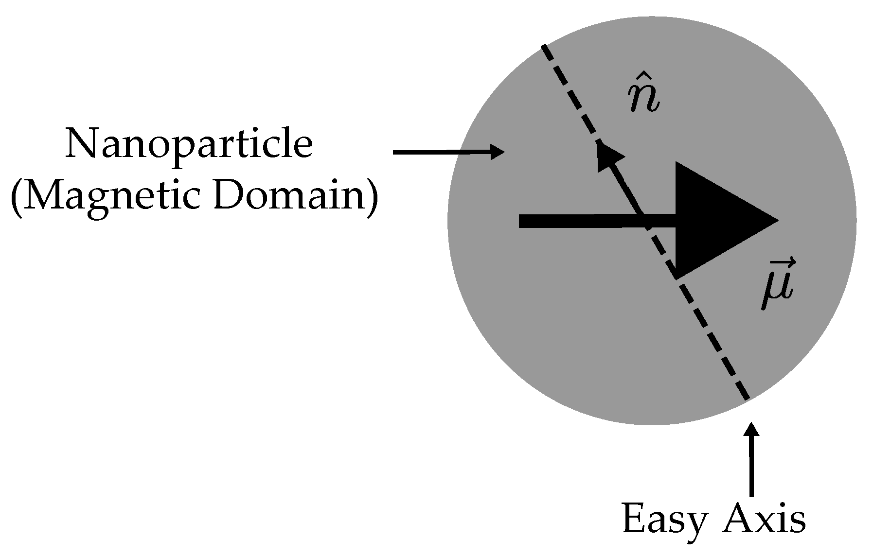
A physical system composed of a set of spherical nanoparticles of equal size, sufficiently spaced so that the interactions between them are negligible and uniformly distributed in a solid matrix in such a way that translations and rotations are forbidden, is considered. Each particle (see Figure 1) is assumed to be a single-magnetic-domain with uniaxial magneto-crystalline anisotropy; as a result, its properties can be characterized through a magnetic moment and an easy axis .
The magnitude of the magnetic moment is equal to the product of (saturation magnetization of the single-domain) with (nanoparticle volume). It is supposed that thermal fluctuations do not change and neither dilate the particle. Likewise, the direction of the easy axis is not affected by the thermal bath nor by internal or external interactions, which means that its initial orientation remains unchanged at all times.
With respect to the foregoing, the simplest Hamiltonian governing the behavior of a magnetic moment in the presence of an external magnetic field is:
where the first term is the anisotropy potential energy that describes the interaction between the magnetic moment and the easy magnetization axis, with the effective magnetic anisotropy constant. Surface and shape contribution to the anisotropy are neglected for simplicity. The second term is the Zeeman potential energy and expresses the coupling between the magnetic moment and the field. Temperature is included using the Metropolis algorithm as indicated in Section 2.3.
2.2. Néel Relaxation
Due to the existence of uniaxial magnetic anisotropy, it is evident from Equation (1) that the magnetic moment has two stable and energetically equal orientations (one of them parallel to the easy axis and the other anti-parallel). These two orientations are separated by an energy barrier equal to and for a given absolute temperature T, there is a probability that the moment spontaneously changes from one direction to the other because of thermal fluctuations. The average time for this change to occur is known as the Néel relaxation time [20] and it is given by the expression:
with a characteristic time of the magnetic solid that takes typical values of s (or less) [21] and Boltzmann’s constant . This equation is only valid for zero or very weak external magnetic fields compared to the anisotropy interaction.
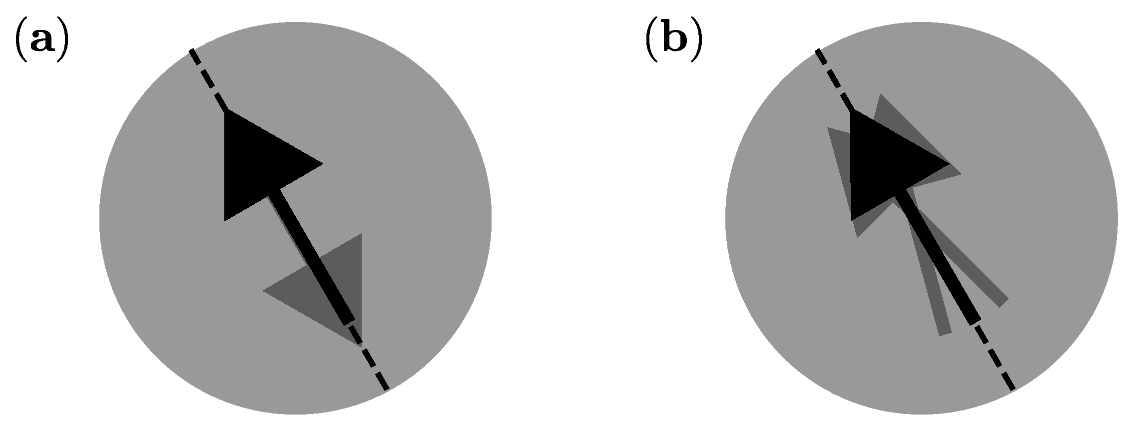
Suppose now that we want to measure the magnetization of a nanoparticle and that the measurement takes a time to be completed. If the measurement time is greater than the Néel time (i.e., ) the result is that the magnetic moment oscillates many times during measurement and therefore the average magnetization is zero (see Figure 2a). Conversely, if this time is smaller than the relaxation time () then the magnetic moment will not oscillate, and it will remain in a blocked state causing the magnetization of the nanoparticle remains well defined (see Figure 2b). The first situation is called superparamagnetic state since the magnetization behaves like that of a paramagnet with macroscopic magnetic moment. The second one is known as a blocked state because the moment remains aligned along a given orientation.
2.3. Metropolis Algorithm Driven by Acceptance Rate
The Metropolis–Hastings algorithm is used to carry out magnetic moment movements and updates along the phase space of the system. For this algorithm, a single Monte Carlo step (MCS) is defined as the elapsed time to visit all the particles (N) in the system and to attempt a new magnetic moment configuration () from a previous one () for every single magnetic moment, by forming in this way the Markov chain. In this scheme, a particle is chosen at random, and the direction of its magnetic moment is perturbed to access a new configuration. If the energy difference between microstates is then the movement is accepted, conversely, if the movement is accepted only with a Boltzmann transition probability given by by comparison with a random number . If the motion is accepted, otherwise is definitively rejected and a new random particle is again selected. The goal of this algorithm, accordingly to a canonical ensemble in contact with a thermal bath as is known in statistical physics, is to make the magnetic moments obey a Boltzmann probability distribution given by:
with E being the eigenvalue of the Hamiltonian of the system (see Equation (1)), Z is the partition function, which serves as normalizing factor, and the vector in phase space stands symbolically for the set of variables describing the degrees of freedom, e.g., . If any of the magnetic moments change from , a new microstate is generated. Thus, the probability density given by Equation (3) describes the statistical weight with which the configuration or microstate occurs in thermal equilibrium [22].
Here, is a Lebesgue density, so is the prior density. In our case, let or be the proposal or instrumental density, i.e., a Markov transition density describing how to go from state to .
To sample phase space, we start from a current or initial state for the magnetic moment with any given random orientation. The trial movement is executed so that the new orientation is close to the old one, with selected inside a cone whose main axis is along (see Figure 3). This update is achieved by means of a double random rotation matrix (visit Appendix A.1) involving a polar angle and an azimuthal one , being the cone aperture. Angles and are chosen randomly from uniform distributions . Thus, and the way as the angles are chosen, makes the Markov matrix Q to be symmetric, i.e., .
A sketch of the algorithm is given in Algorithm 1, where is called the acceptance/rejection probability. With this election, the principle of detailed balance is fulfilled and the ratio of transition probabilities depends only on the energy change .
| Algorithm 1 Metropolis–Hastings Algorithm. |
| Given the current state , then: |
|
| Return and . |
In discrete event-based Monte Carlo simulations on classical magnetic systems, new orientations of the magnetic moments are chosen completely at random, i.e., instead of , and independent on the initial state . The consequence of this is that the system always exhibits a superparamagnetic behavior regardless of the temperature value, as Dimitrov and Wysin [19] warned in their paper, since the system can rapidly escape from metastable states responsible for magnetic hysteresis. Please note that is a parameter that has not been specified so far, and it is the one responsible for controlling the convergence rate of the algorithm and how the exploration of the phase space is performed. If it is too small most of the moves will be accepted and vice versa.
The undesired effect of having the system always in a superparamagnetic regime can be overcome precisely through a proper handling of the parameter. To do so we try to reproduce a dynamic similar to that of the LLG framework (where the system always evolves and explores likely microstates), by stating that must be modified in a self-adaptive manner such that the phase space is sampled at a constant rate. This is achieved by including an additional acceptance rate , which is calculated by counting the number of accepted movements in a large enough number of MC steps . is thus calculated and is updated every single Monte Carlo step (MCS). Thus, the cone aperture is adjusted so that statistically remains constant as much as possible within certain tolerance range during the simulation of any curve. For such purposes, it is imposed that all the particles are selected and attempted to be perturbed so that a specific influences equally the behavior of the set (see Algorithm 2).
| Algorithm 2 Main Algorithm. |
| Set the initial conditions: magnetic field, temperature, magnetic moments orientations, the easy axes orientations and so on. |
|
The self-adaptation process of is as follows (see Algorithm 3): an initial value for is chosen, namely a corresponding to the target acceptance rate we pretend to achieve, and then the acceptance rate is calculated after a Monte Carlo step. If , which means more accepted movements (this happens when is small), then is increased by taking care that the maximum value of is not exceeded. On the other hand, if , which means less accepted movements (this happens when is big), then is reduced by . We can do this because Q is not uniquely determined and some arbitrariness in the explicit choice of it remains.
| Algorithm 3 Cone Aperture Update. |
|
With the election of such percentages, i.e., with for the confidence interval of and for the increase/decrease of the cone aperture , we managed to guarantee . For other percentages, in our tests, a stability in the acceptance rate was not achieved. In Appendix A.2 we show the results of some tests and diagnostics over this algorithm, including autocorrelation plots, effective sample size and thin size.
3. Results and Discussion
In our simulation we used a total number of particles with magnetic anisotropy constant kJm and radius of nm. A saturation magnetization per particle kAm corresponding to magnetite [24] and for the ensemble were employed. Additionally, for all experiences the easy axes were randomly oriented. Numerical experiments are explained and discussed below.
3.1. Magnetization, Acceptance Rate and Cone Aperture vs. Magnetic Field
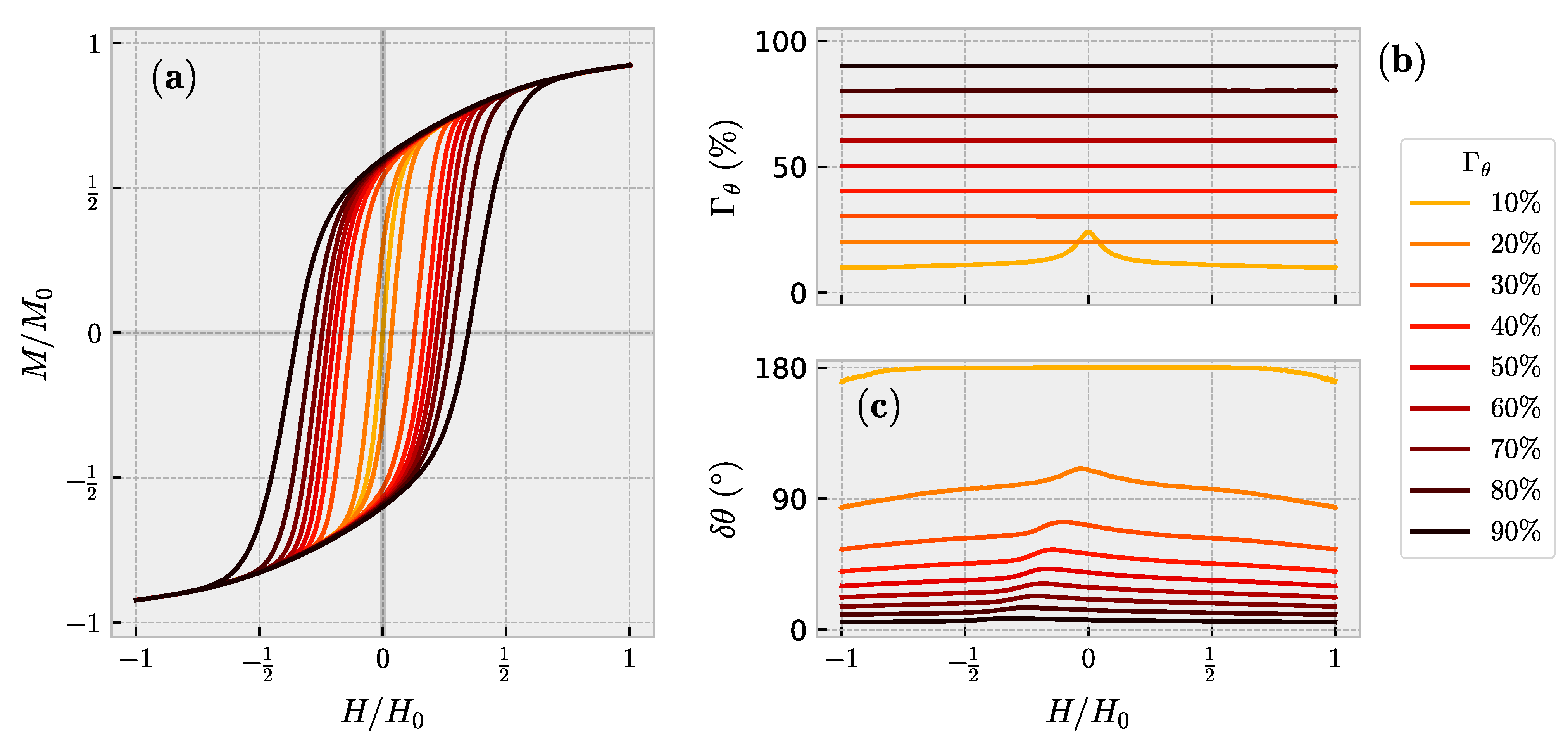
This section explores the dependence of magnetization both as function of a time-dependent field and the respective MCS dependence when a constant magnetic field is applied. At the beginning of each time-dependent field experience, all the magnetic moments are randomly oriented, and they are thermalized until saturation. To accomplish this initial state, 2000 MCS are required. For curves such as those shown in Figure 4, 200 points are used and a magnetic field in the z-direction is chosen according to the rule:
with kAm (or 500 Oe) the field amplitude and the time variable given in MCS units. This particular choice is made since the magnetic hysteresis cycles are symmetrical and it is enough to calculate the upper branch, so a half oscillation in the field is only necessary, whereas the lower branch is obtained by simultaneously reflecting the first one with respect to the H (or x) and M (or y) axes. At each i-th time value, a constant field is assumed, and the evolution is performed using the Metropolis algorithm. Half of the total MCS, namely , are used to thermalize the system at a given new field value and the other half is used for data collection and averages calculation purposes. A total number of MCS was employed at every point per experiment.
Figure 4 shows the results for (a) the reduced magnetization , (b) the acceptance rate and (c) the cone aperture as a function of the reduced magnetic field at K. Each point on the curve of magnetization is the result of averaging the magnetic moments of the particles in the field-direction during data acquisition. The same averaging process is performed for and (see Section 2.3). All curves are in addition the result of configurational averages performed over 100 independent numerical experiments.
As is observed in Figure 4a, the system exhibits hysteresis for values of above , whereas for of acceptance the system behaves as a superparamagnet. As the acceptance rate increases above both the coercivity and the squareness of the loop increase. It is remarkable the degree of control on the acceptance rate above as can be observed in Figure 4b, which is constant for all the range of values of the external field. Only for of acceptance a noticeable variation is observed only at low fields. In Section 3.2 we discuss this feature where both the temperature and the fact of having the system in a superparamagnetic state are key factors to understand such phenomenology.
As concerns to Figure 4c, for higher values of , the angular parameter of the cone aperture is smaller. This fact means that the system remains confined at metastable states as long as the movements are strongly bounded. This is clearly demonstrated by looking at the cycle for where the hysteresis is the biggest one and the coercive force is also the strongest one, which is a clear indicative of the high degree of metastability. Likewise, the peaks observed for are the ones where the switching fields take place. For such fields, the cone aperture becomes greater as a physical mechanism to allow magnetization reversal. In addition, remanence (at zero field) is due to the coupling of the magnetic moments along that component of the easy axes favoring the direction of the applied field. On the other hand, for low values, the aperture cone is greater, which means that between step and step, the magnetic moments can rotate more freely, performing broader trajectories in phase space and therefore they can easily escape from metastable states so the magnetic moments remain in an alternating regime giving rise to a zero average magnetization (see Section 2.2). As a result, no hysteresis is observed, and the superparamagnetic state is finally established.
The progressive disappearance of coercivity as the acceptance rate decreases, is consistent with a continuous transition from a blocked state to a superparamagnetic one. In this sense, blocked states are characterized by small values of the cone aperture , which is in agreement with what is expected for a so-called “blocked” state. In contrast, at zero coercivity (), the widest cone apertures are consistent to what is expected for a “superparamagnetic” regime. Such a gradual disappearance of coercivity coincides with typical observations of the behavior of curves as a function of the measurement time , in which the state of the nanoparticle (superparamagnetic or blocked) depends on the comparison between the measurement time and the Néel relaxation time (see Section 2.2). Thus, at first glance, for a given system, our acceptance rate , which is indeed a frequency of acceptance, seems to be related to the reciprocal of the measurement time, i.e., . This fact is endorsed by the Néel-Arrhenius relationship observed between the remanence () and for , i.e., the expression is fulfilled by taking the variable . We want to recall at this point that the maximum number of MCS was kept constant. As we show below, very small values of imply a high rate of rejections, and therefore phase space sampling is not so efficient, and averages are not reliable.
Another interpretation could be in turn one for which the parameter goes proportional to . i.e., and the measurement time refers to the number of MCS used for data acquisition. Thus, if the MCS number is kept constant, as in our case, the interplay between blocked and superparamagnetic states can be achieved by tuning or equivalently . Thus, high values of give rise to the compliance of favoring the appearance of blocked states, as is effectively observed. Conversely, small values of will favor the inequality and superparamagnetic states will be observed. In both scenarios, the role played by recovers the behavior observed in the superparamagnetic theory.
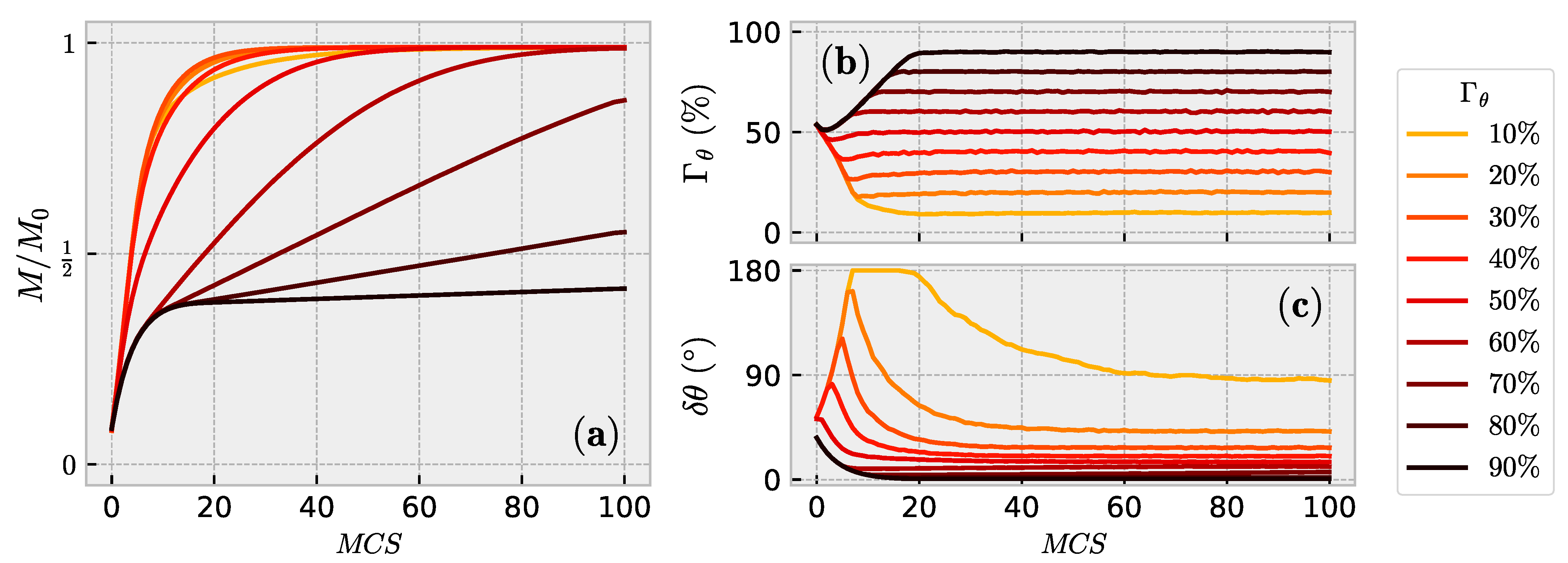
Concerning the use of a constant field and the time dependence of the observables, results are summarized in Figure 5. In this case, the time dependence in MCS units is obtained for (a) the reduced magnetization, (b) the acceptance rate and (c) the cone aperture angle at K. In this case, the time evolution of the magnetization process was obtained at a constant field of 200 kAm (or 2500 Oe) starting from an initial configuration of magnetic moments randomly distributed. Curves are in turn the configurational average over 100 experiments statistically independent.
Figure 5a shows the effect of the acceptance rate in the magnetization process under an applied field. Concretely, for small values of , the system can easily reach the saturation state within a small range of MCS. This behavior can be ascribed to the fact that more microstates compatible with those where the alignment of the magnetic moments with the field are generated as the cone aperture is increasingly wider. In particular, for up to , magnetization curves seem to overlap, and discrepancies in the magnetization mechanism, are only observable for greater percentages. Moreover, the system progressively becomes magnetically harder making the saturation state more difficult to reach as the acceptance rate increases.
Figure 5b shows the time evolution of the parameter. In all cases, the system seems to initiate its dynamics at , related to the random initial configuration of the magnetic moments. Once the dynamics starts, evolves toward the expected values , initially determined, reaching steady states within the first 20 MCS. Analogously, the time evolution of the cone aperture angle is shown in Figure 5c. Here, an initial value of ° was defined. In this case, convergence is also achieved but in a different fashion, passing through a well-defined peak, dealing with the particular mechanism the system follows in phase space during the magnetization process for every value considered.
3.2. Superparamagnetic Behavior and Temperature Dependence
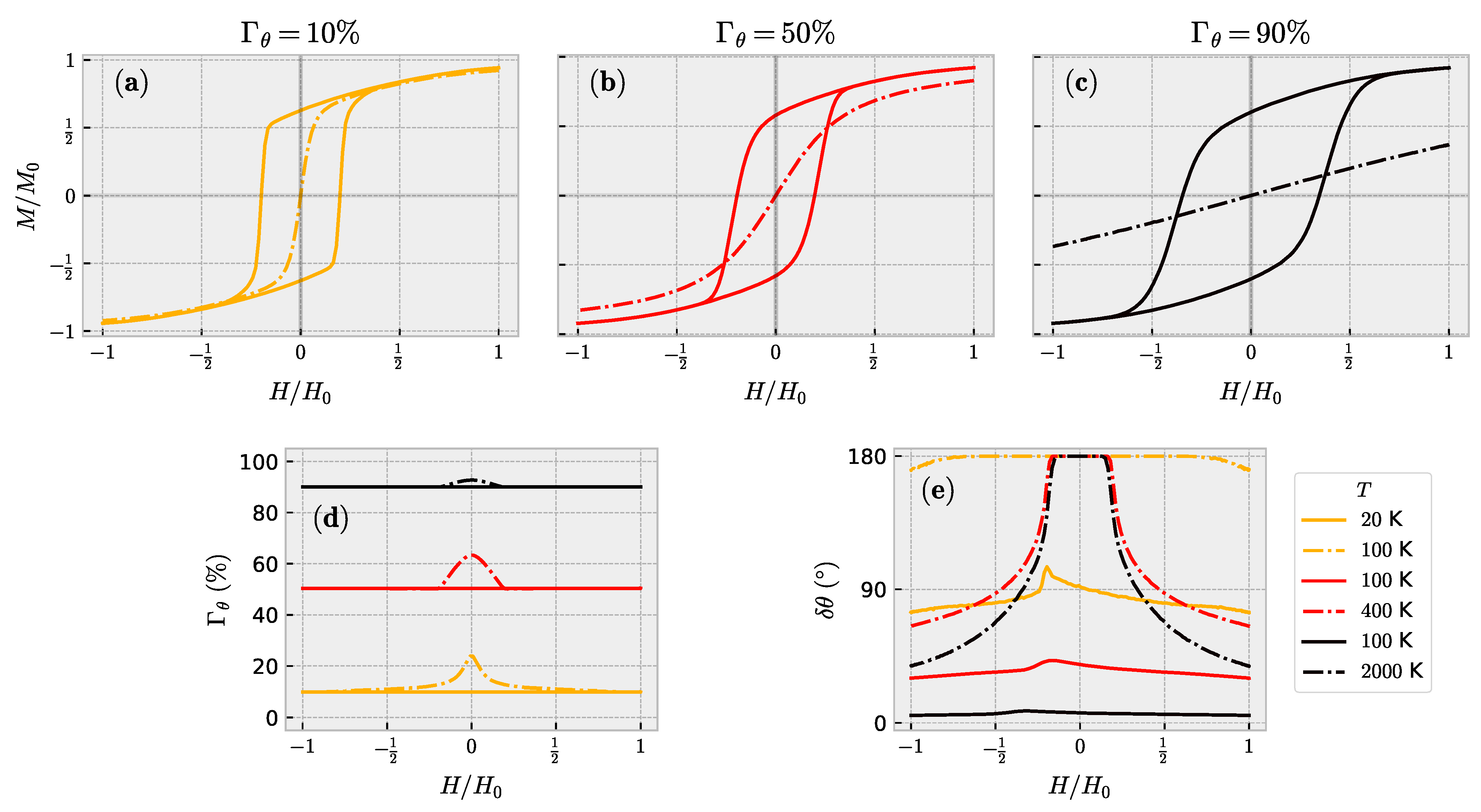
Figure 6 summarizes the circumstances under which both the blocked behavior (that one characterized by open hysteresis loops drawn with solid lines) and the superparamagnetic state (dashed lines with no hysteresis) take place at different temperatures. Results are shown in Figure 6a–c for percentages of , and , respectively. In Figure 6d,e the corresponding behaviors of the acceptance rate and the cone aperture angle are respectively plotted.
Temperature is a key factor in determining the behavior of acceptance rate and the cone aperture. This is clearly demonstrated in Figure 6d,e. As temperature increases along with its respective fluctuations, new microstates, which are not energetically favorable at low temperatures, can now be achieved. An interesting feature occurs along the continuous transition at some blocking temperature , which is dependent on the acceptance rate, for which the system passes from a blocked state with a coercive force different from zero to a superparamagnetic one. At this last stage, the high fluctuations in the orientations of the magnetic moments at low fields, make that exhibits a peak and concomitantly reaches the maximum value (180°), which makes difficult, under the temperature and field conditions, to equilibrate the desired value of . The appearance of the peak for , above the target value , is due to the increment in the new movement acceptance because of those new microstates achieved during the self-regulation process of . Blocked states require comparatively small values contrary to those of the superparamagnetic state (see the comparison between continuous and dashed lines in Figure 6e).
More specifically, for low fields close to zero, the orientations energetically favorable are those dictated by the easy anisotropy axes, which are doubly degenerated. Thus, thermal fluctuations are the ones responsible for the moments to alternate not only along such directions but also in between, giving rise to the excess of acceptance rate observed. In consequence an average magnetization close to zero is obtained.
In contrast to the low-field scenario, at high fields (positive or negative) the most likely and privileged orientations are those satisfying the alignment criterion between the magnetic moments and the applied field. Thus, orientations energetically not favorable, although thermally probable, represent a smaller population than those corresponding to zero field. This is the reason an excess in the acceptance rate is not observed. Additionally, we want to stress that our results also show that the superparamagnetic state is achieved at different blocking temperatures depending on . This fact leads us to conclude that the acceptance rate must be related to the measurement time involved in the following expression for the blocking temperature (see Section 2.2):
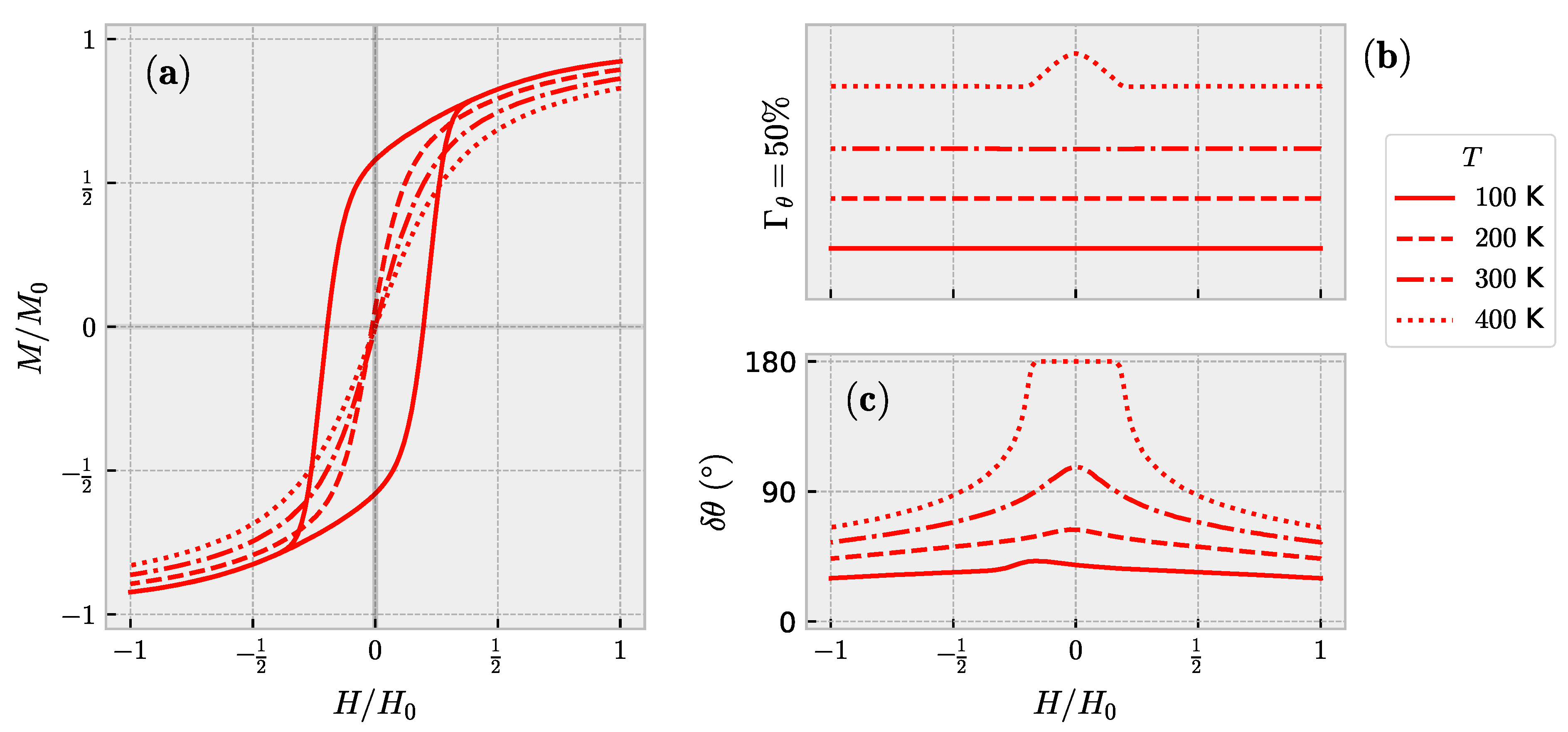
To validate the above reasoning, Figure 7 shows the curves for and for some selected temperatures. As observed, some superparamagnetic states are possible to reproduce with constant acceptance rate, i.e., sampling of the phase space occurs at constant speed, except for the one at the highest temperature (400 K). On this basis we can point out that when temperature is high enough the Boltzmann distribution makes any orientation to null fields highly probable, and the acceptance rate increases. If temperature increases indefinitely, all the microstates become equiprobable for any applied field, and the acceptance rate is expected to increase up to . Such a limit case is inferred from the Boltzmann probability distribution for .
4. Conclusions
In this work, we have implemented a novel algorithm, which allows reproducing both the blocked and superparamagnetic states of a system of independent magnetic nanoparticles with uniaxial magneto-crystalline anisotropy randomly distributed. The method presented is based on the Markov chain Monte Carlo method with Metropolis–Hastings algorithm for which the magnetic moments movements are proposed to be accepted at a constant rate as phase space is sampled. Consequently, the aperture of the rotations in the updates of the magnetic moments must be self-regulated. Isotherms of curves show that a constant acceptance rate makes cone aperture of the rotations of the magnetic moments must lie below certain upper bounds. The amplitude of such an aperture is the responsible one for the occurrence of either blocked or superparamagnetic states.
For high values of , much more microstates must be accepted, so the upper bound for must decrease to satisfy the constant acceptance rate condition. In this case, exploration of the phase space is slow, and it takes time for the system to find states of relaxation. In contrast, for small values of , much more microstates are rejected, so the upper bound for must increase. In this case, exploration of the phase space is faster, and the system relaxes more easily. Concomitantly, temperature plays a key role in these processes since it helps to make more likely energetically unfavorable events. This causes an extra excess in the acceptance rate and the cone aperture must be readjusted to equilibrate such an unbalance. Additionally, our results allow also to show, from the set of isotherms in the curves, that the election of a predefined acceptance rate can give rise to different blocking temperatures. This fact leads us to conclude that the acceptance rate must be related to the measurement time.
Finally, a value of implies that most of the movements of the magnetic moments are rejected so the exploration of the phase space to find representative microstates is not efficient. In other words, importance sampling is incomplete to guarantee reliable averages of observables. For this reason, we do not recommend using such small values of .
Author Contributions
Conceptualization, J.C.Z. and J.R.; methodology, J.C.Z.; software, J.C.Z.; validation, J.C.Z. and J.R.; formal analysis, J.C.Z. and J.R.; investigation, J.C.Z.; data curation, J.C.Z.; writing—original draft preparation, J.C.Z.; writing—review and editing, J.R.; visualization, J.C.Z.; supervision, J.R.; funding acquisition, J.R. All authors have read and agreed to the published version of the manuscript.
Funding
J.R. acknowledges University of Antioquia for the exclusive dedication program. Financial support was provided by the CODI-UdeA 2020-34211 Simulmag2 project.
Institutional Review Board Statement
Not applicable.
Informed Consent Statement
Not applicable.
Data Availability Statement
Data presented in this study are available in GitHub.
Conflicts of Interest
The authors declare no conflict of interest.
Appendix A
Appendix A.1. Magnetic Moment Rotation
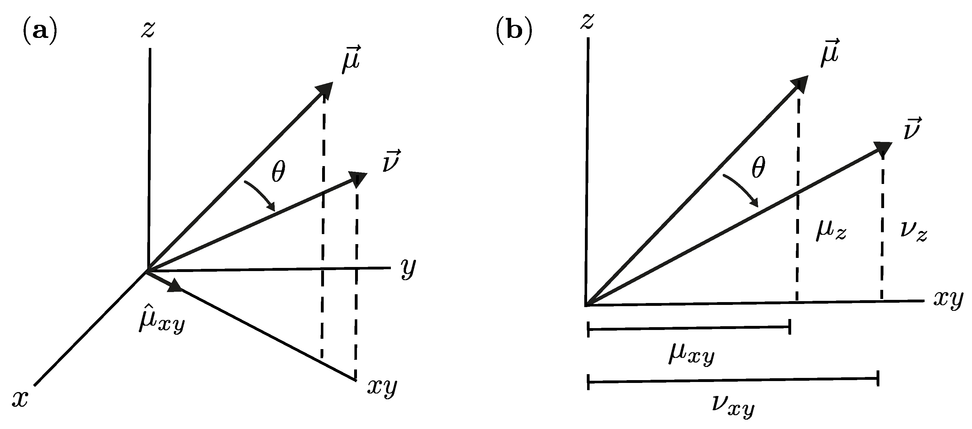
As mentioned in Section 2.3, the trial movement of the magnetic moment, named , is obtained by means of a double rotation R over , characterized first by a polar angle and followed by an azimuthal one , both of them of random nature. Based on Figure 3, the polar angle rotation is sketched in Figure A1, where is the result of that first step.
Figure A1.
Polar rotation of the magnetic moment. (a) the three-dimensional (3D) representation and (b) the two-dimensional (2D) representation.
Figure A1.
Polar rotation of the magnetic moment. (a) the three-dimensional (3D) representation and (b) the two-dimensional (2D) representation.

In the usual three-dimensional (3D) representation and or in two dimensions (2D) and , with and being the projections of y on the -plane respectively. Hence, is given by the clockwise transformation rule:
or
Based on Figure A1a and returning to the 3D representation we have with a unitary vector in the direction of in plane. By combining with the set of Equation (A2), we have the expression that allows us to calculate the rotation of the vector a polar angle :
Once the polar rotation is done, then the azimuthal rotation occurs for a given random angle . This can be done using the Rodrigues rotation formula to rotate the vector around an angle to finally obtain (see Figure 3):
note the unitary vector . Equations (A3) and (A4) summarize the transformation with the rotation matrix that is not explicitly specify.
Appendix A.2. Algorithm Testing and Diagnostics
Markov chain Monte Carlo samplers are known for their highly correlated draws since every posterior sample is extracted from a previous one. To evaluate this issue in the MH algorithm, we have computed the autocorrelation function for the magnetic moment of a single particle, and we have also studied the effective sample size, or equivalently the number of independent samples to be used to obtained reliable results. In addition, we evaluate the thin sample size effect, which gives us an estimate of the interval time (in MCS units) between two successive observations to guarantee statistical independence.
To do so, we compute the autocorrelation function between two magnetic moment values and given a sequence of n elements for a single particle:
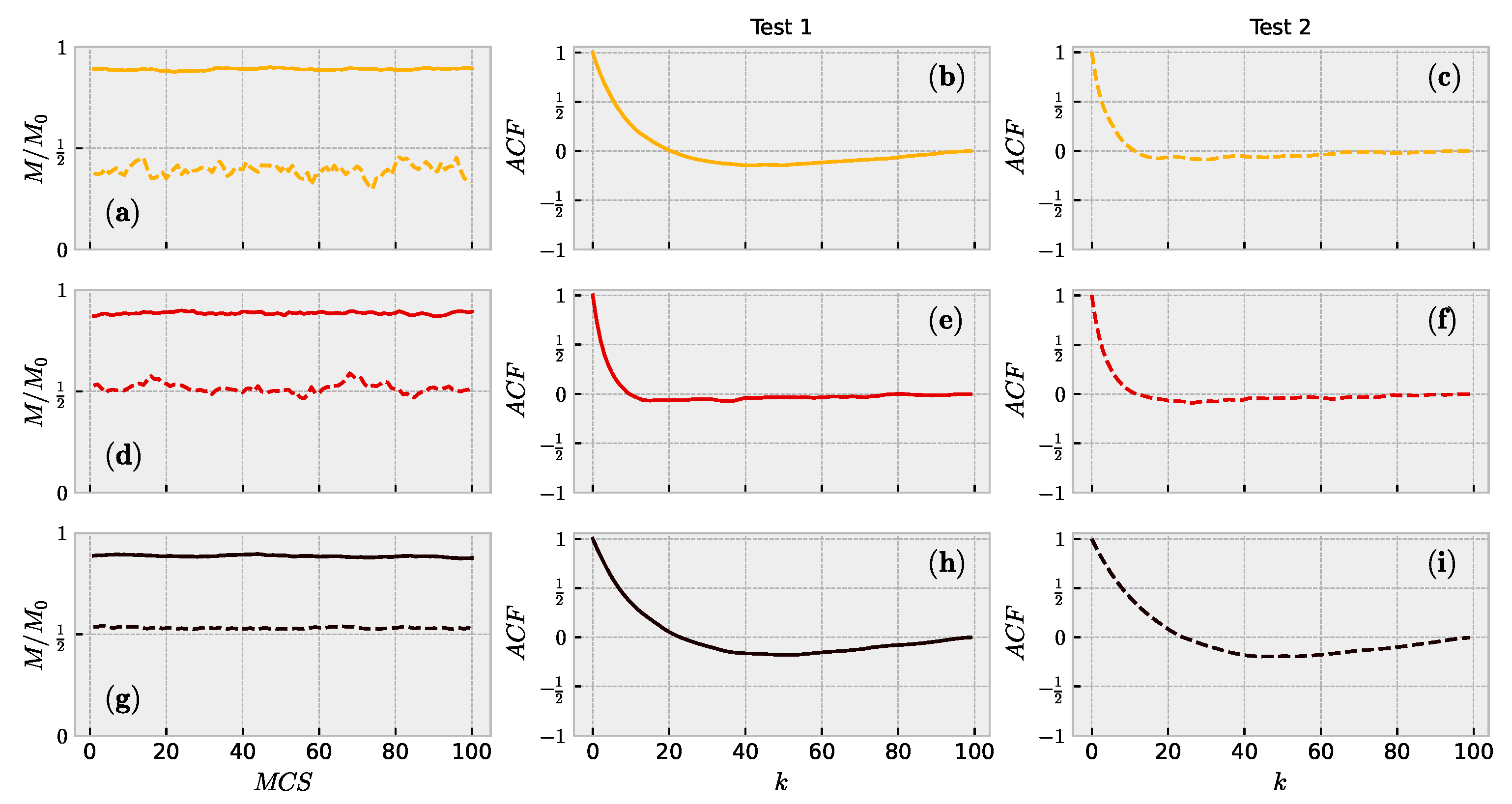
where is the autocovariance, is the variance, and k is the time interval between two observations. Results of the for several acceptance rates and two different values of the external applied field compatible with the curves of Figure 4a and a particle with easy axis oriented 60°with respect to the field, are shown in Figure A2. Let Test 1 be the experiment associated with an external field close to the saturation field, i.e., , and let Test 2 be the experiment for another field, i.e., .
Figure A2.
(a,d,g) single particle reduced magnetization as a function of the Monte Carlo steps for percentages of acceptance of (orange), (red) and (black), respectively. (b,e,h) show the autocorrelation function for the magnetic field and (c,f,i) for .
Figure A2.
(a,d,g) single particle reduced magnetization as a function of the Monte Carlo steps for percentages of acceptance of (orange), (red) and (black), respectively. (b,e,h) show the autocorrelation function for the magnetic field and (c,f,i) for .

Figure A2a,d,g show the dependence of the reduced magnetization with the Monte Carlo steps. As is observed, magnetization is distributed around a well-defined mean value. As we have already mentioned in Section 3, the half of the total number of Monte Carlo steps has been considered for averaging purposes. These graphs confirm that such an election is a good one and it could even be less.
Figure A2b,c show the results of the autocorrelation function for different k time intervals between successive measurements and for an acceptance rate of . The same for Figure A2e,f with an acceptance rate of , and Figure A2h,i with an acceptance rate of . Results for smaller than show the onset of statistical independence from around . Above this value the function goes to zero. In the case of a higher value is needed. Thus, the values obtained suggest statistical independence every 20 samples or even below. This is a good estimate of the thinning process.
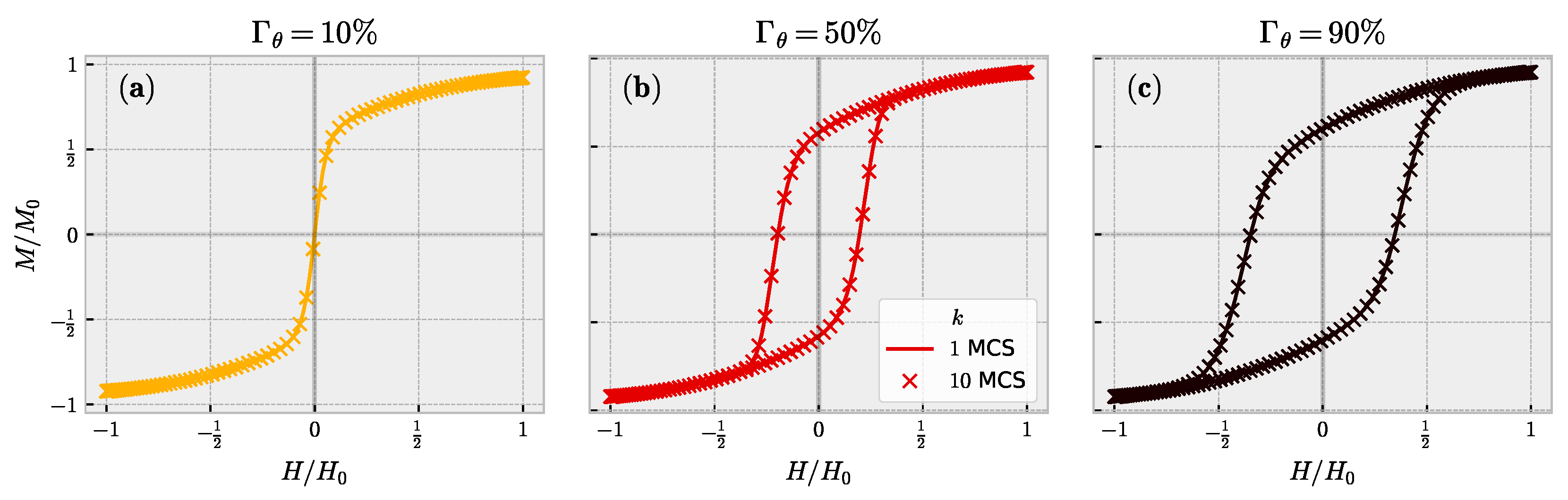
On the other hand, Figure A3 shows the results of the reduced magnetization as a function of the reduced field for the same values from above. As is shown, two scenarios have been considered. One without delay by taking the measurements every single MCS, and the other one every 10 MCS. No differences are noticed. So, we can conclude that despite the degree of correlation, this fact does not alter the value of our observable, which is the magnetization. W. A. Link and M. J. Eaton (2012) [25] suggest that doing a sequence thinning is often unnecessary and inefficient as it can reduce the precision of the Markov chain.
Figure A3.
H-dependence of the reduced magnetization for percentages of acceptance of (a) , (b) and (c) . Results without delay (i.e., every 1 MCS, which means consecutive measurements) are drawn with solid lines and those with a delay of 10 MCS with an x-marker.
Figure A3.
H-dependence of the reduced magnetization for percentages of acceptance of (a) , (b) and (c) . Results without delay (i.e., every 1 MCS, which means consecutive measurements) are drawn with solid lines and those with a delay of 10 MCS with an x-marker.

Results for the tests yield values of . This tells us that at least the half of the total number of samples is suitable for the inference of the observables. Such a value endorses our election for the cut-off time (50 MCS) and the total number of 100 MCS.
References
- Stoner, E.C.; Wohlfarth, E.P. A mechanism of magnetic hysteresis in heterogeneous alloys. Philos. Trans. R. Soc. London Ser. A. 1948, 240, 599. [Google Scholar] [CrossRef]
- Néel, L. Theorie du trainage magnetique des ferromagnetiques en grains fins avec applications aux terres cuites. Ann Geophys. 1949, 5, 99. [Google Scholar]
- Brown, W.J. Thermal Fluctuations of a Single-Domain Particle. Phys. Rev. 1963, 130, 1677. [Google Scholar] [CrossRef]
- Rümenapp, C.; Gleich, B.; Haase, A. Magnetic nanoparticles in magnetic resonance imaging and diagnostics. Pharm. Res. 2012, 29, 1165–1179. [Google Scholar] [CrossRef]
- Fatima, H.; Charinpanitkul, T.; Kim, K.-S. Fundamentals to Apply Magnetic Nanoparticles for Hyperthermia Therapy. Nanomaterials 2021, 11, 1203. [Google Scholar] [CrossRef] [PubMed]
- Giustini, A.J.; Petryk, A.A.; Cassim, S.M.; Tate, J.A.; Baker, I.; Hoopes, P.J. Magnetic Nanoparticle Hyperthermia in Cancer Treatment. Nano LIFE 2010, 1, 17–32. [Google Scholar] [CrossRef] [PubMed]
- Akbarzadeh, A.; Samiei, M.; Davaran, S. Magnetic nanoparticles: Preparation, physical properties, and applications in biomedicine. Nanoscale Res. Lett. 2012, 7, 144. [Google Scholar] [CrossRef] [Green Version]
- García-Palacios, J.L.; Lázaro, F.J. Langevin-dynamics study of the dynamical properties of small magnetic particles. Phys. Rev. B 1998, 58, 14937. [Google Scholar] [CrossRef] [Green Version]
- Shah, S.A.; Reeves, D.B.; Ferguson, R.M.; Weaver, J.B.; Krishnan, K.M. Mixed Brownian alignment and Néel rotations in superparamagnetic iron oxide nanoparticle suspensions driven by an ac field. Phys. Rev. B 2015, 92, 094438. [Google Scholar] [CrossRef] [Green Version]
- Shasha, C.; Krishnan, K.M. Nonequilibrium dynamics of magnetic nanoparticles with applications in biomedicine. Adv. Mater. 2020, 33, 1904131. [Google Scholar] [CrossRef]
- Tran, N.L.; Tran, H.H. Role of the poly-dispersity and the dipolar interaction in magnetic nanoparticle systems: Monte Carlo study. J. Non-Cryst. Solids 2011, 357, 996–999. [Google Scholar] [CrossRef]
- Schaller, V.; Wahnström, G.; Sanz-Velasco, A.; Enoksson, P.; Johansson, C. Monte Carlo simulation of magnetic multi-core nanoparticle. J. Magn. Magn. Mater. 2009, 321, 1400–1403. [Google Scholar] [CrossRef]
- Khodadadian, A.; Noii, N.; Parvizi, M.; Abbaszadeh, M.; Wick, T.; Heitzinger, C. A Bayesian estimation method for variational phase-field fracture problems. Comput. Mech. 2020, 66, 827–849. [Google Scholar] [CrossRef] [PubMed]
- Mirsiand, S.; Khodadadiana, A.; Hedayatid, A.; Manzour-ol-Ajdadd, A.; Kalantarinejadd, R.; Heitzingera, C. A new method for selective functionalization of silicon nanowire sensors and Bayesian inversion for its parameters. Biosens. Bioelectron. 2019, 142, 111527. [Google Scholar] [CrossRef] [PubMed]
- Khodadadian, A.; Stadlbauer, B.; Heitzinger, C. Bayesian inversion for nanowire field-effect sensors. J. Comput. Electron. 2020, 19, 147–159. [Google Scholar] [CrossRef] [Green Version]
- Minson, S.E.; Simons, M.; Beck, J.L. Bayesian inversion for finite fault earthquake source models I—Theory and algorithm. Geophys. J. Int. 2013, 194, 1701–1726. [Google Scholar] [CrossRef] [Green Version]
- Cardiff, M.; Kitanidis, P.K. Bayesian inversion for facies detection: An extensible level set framework. Water Resour. Res. 2009, 45, W10416. [Google Scholar] [CrossRef]
- Melenev, P.V.; Raikher, Y.L.; Rusakov, V.V.; Perzynski, R. Time quantification for Monte Carlo modeling of superparamag-netic relaxation. Phys. Rev. B 2012, 86, 104423. [Google Scholar] [CrossRef]
- Dimitrov, D.A.; Wysin, G.M. Magnetic properties of superparamagnetic particles by a Monte Carlo method. Phys. Rev. B 1996, 54, 9237. [Google Scholar] [CrossRef] [Green Version]
- Dieckhoff, J.; Eberbeck, D.; Schilling, M.; Ludwig, F. Magnetic-field dependence of Brownian and Néel relaxation times. J. Appl. Phys. 2016, 119, 043903. [Google Scholar] [CrossRef]
- Omelyanchik, A.; Salvador, M.; D’Orazio, F.; Mameli, V.; Cannas, C.; Fiorani, D.; Musinu, A.; Rivas, M.; Rodionova, V.; Varvaro, G.; et al. Magnetocrystalline and Surface Anisotropy in CoFe2O4 Nanoparticles. Nanomaterials 2020, 10, 1288. [Google Scholar] [CrossRef] [PubMed]
- Binder, K.; Heermann, D.W. Monte Carlo Simulation in Statistical Physics. An Introduction, 5th ed.; Springer: Berlin, Germany, 2010; pp. 5–19. [Google Scholar]
- Stuart, A.M. Inverse problems: A Bayesian perspective. Acta Numer. 2010, 19, 451–559. [Google Scholar] [CrossRef] [Green Version]
- Rosensweig, R.E. Heating magnetic fluid with alternating magnetic field. J. Magn. Magn. Mater. 2002, 252, 370–374. [Google Scholar] [CrossRef]
- Link, W.A.; Eaton, M.J. On thinning of chains in MCMC. Br. Ecol. Soc. 2012, 3, 112–115. [Google Scholar] [CrossRef]
- Gatsonis, C.; Carriquiry, A.; Kass, R.E.; Gelman, A.; Higdon, D.; Pauler, D.K.; Verdinelli, I. Case Studies in Bayesian Statistics, 1st ed.; Springer: New York, NY, USA, 2002; Volume 6, pp. 214–215. [Google Scholar]
Figure 1.
Magnetic nanoparticle structure.

Figure 2.
Representation of the superparamagnetic (a) and blocked (b) regimes under Néel relaxation.
Figure 2.
Representation of the superparamagnetic (a) and blocked (b) regimes under Néel relaxation.

Figure 3.
Cone used to choose the random motion of the magnetic moment.

Figure 4.
Reduced magnetization (a), acceptance rate (b) and cone aperture (c) as a function of the external magnetic field.
Figure 4.
Reduced magnetization (a), acceptance rate (b) and cone aperture (c) as a function of the external magnetic field.

Figure 5.
(a) Reduced magnetization, (b) acceptance rate and (c) cone aperture as a function of the Monte Carlo steps.
Figure 5.
(a) Reduced magnetization, (b) acceptance rate and (c) cone aperture as a function of the Monte Carlo steps.

Figure 6.
Reduced magnetization for percentages of acceptance of (a) , (b) and (c) , (d) acceptance rate and (e) cone aperture depending on the external field for different temperature values. At low temperatures magnetic hysteresis (solid lines) is observed whereas for high enough temperatures a superparamagnetic behavior occurs (dashed lines).

Figure 7.
(a) Reduced magnetization, (b) acceptance rate and (c) cone aperture as a function of the external magnetic field for . Blocked and superparamagnetic behaviors are obtained depending on temperature.
Figure 7.
(a) Reduced magnetization, (b) acceptance rate and (c) cone aperture as a function of the external magnetic field for . Blocked and superparamagnetic behaviors are obtained depending on temperature.

Publisher’s Note: MDPI stays neutral with regard to jurisdictional claims in published maps and institutional affiliations. |
© 2021 by the authors. Licensee MDPI, Basel, Switzerland. This article is an open access article distributed under the terms and conditions of the Creative Commons Attribution (CC BY) license (https://creativecommons.org/licenses/by/4.0/).
Share and Cite
MDPI and ACS Style
Zapata, J.C.; Restrepo, J. Self-Adaptive Acceptance Rate-Driven Markov Chain Monte Carlo Method Applied to the Study of Magnetic Nanoparticles. Computation 2021, 9, 124. https://0-doi-org.brum.beds.ac.uk/10.3390/computation9110124
AMA Style
Zapata JC, Restrepo J. Self-Adaptive Acceptance Rate-Driven Markov Chain Monte Carlo Method Applied to the Study of Magnetic Nanoparticles. Computation. 2021; 9(11):124. https://0-doi-org.brum.beds.ac.uk/10.3390/computation9110124
Chicago/Turabian StyleZapata, Juan Camilo, and Johans Restrepo. 2021. "Self-Adaptive Acceptance Rate-Driven Markov Chain Monte Carlo Method Applied to the Study of Magnetic Nanoparticles" Computation 9, no. 11: 124. https://0-doi-org.brum.beds.ac.uk/10.3390/computation9110124
Note that from the first issue of 2016, this journal uses article numbers instead of page numbers. See further details here.