
Data Analysis and Symbolic Regression Models for Predicting CO and NOx Emissions from Gas Turbines


Department Applied Mathematics and Computer Modelling, National University of Oil and Gas “Gubkin University”, 65, Leninsky Prospekt, 119991 Moscow, Russia
*
Author to whom correspondence should be addressed.
†
These authors contributed equally to this work.
Computation 2021, 9(12), 139; https://0-doi-org.brum.beds.ac.uk/10.3390/computation9120139
Submission received: 15 November 2021
/
Revised: 5 December 2021
/
Accepted: 9 December 2021
/
Published: 13 December 2021
(This article belongs to the Special Issue Explainable Computational Intelligence, Theory, Methods and Applications)
Abstract
:Predictive emission monitoring systems (PEMS) are software solutions for the validation and supplementation of costly continuous emission monitoring systems for natural gas electrical generation turbines. The basis of PEMS is that of predictive models trained on past data to estimate emission components. The gas turbine process dataset from the University of California at Irvine open data repository has initiated a challenge of sorts to investigate the quality of models of various machine learning methods to build a model for predicting CO and NOx emissions depending on ambient variables and the parameters of the technological process. The novelty and features of this paper are: (i) a contribution to the study of the features of the open dataset on CO and NOx emissions for gas turbines, which will enable one to more objectively compare different machine learning methods for further research; (ii) for the first time for the CO and NOx emissions, a model based on symbolic regression and a genetic algorithm is presented—the advantage of this being the transparency of the influence of factors and the interpretability of the model; (iii) a new classification model based on the symbolic regression model and fuzzy inference system is proposed. The coefficients of determination of the developed models are: for NOx emissions, for CO emissions.
1. Introduction
One of the essential sources of harmful pollutants (NOx and CO) released in the atmosphere is the combustion process in the power industry. NOx is a generic term for the emission family of nitrogen dioxide (NO2) and nitric oxide (NO), which are produced from the reaction of nitrogen and oxygen gases in the air during combustion. There are three main mechanisms for the formation of nitrogen oxides during gas combustion: “thermal”, “fast”, and “fuel” NOx. In accordance with the thermal theory, the rate of NOx formation depends on the temperature of the combustion zone, on the residence time of the combustion products in the high-temperature zone, and on the oxygen concentration in this zone. “Fast” NOx are formed in the initial region of the flame front in the temperature range of 1000–1500 K. “Fuel” NOx are formed from nitrogen-containing fuel compounds. Since natural gas does not contain nitrogen compounds, or contains them in very small quantities, only the first two mechanisms of NOx formation lead to emissions in gas turbines which are limited by strict environmental regulations. According to Industrial Emissions Directive, the flue gas concentrations of NOx and CO must be continuously measured from each combustion plant exceeding a total capacity of 100 MW. Predictive emission models do not require significant initial and ongoing financial costs to help prove the reliability of continuous measurements. An overview of the history of PEMS development as well as the regulatory framework can be found in [1]. There are two main approaches to model building for PEMS: analytical equations derived from the laws of thermodynamics, mass and energy balance, and data-driven models, including statistical and machine learning methods. The publication of the dataset in the open data repository of the University of California, Irvine, School of Information and Computer Science [2] in 2019 allowed researchers to start open discussion on the features of data and the quality of models derived from various machine learning methods to predict CO and NOx emissions.
In [3], the dataset under study was presented for the first time and a description of its main statistical characteristics was given. The dataset was collected for 5 years which contained 36,733 instances of 11 sensor measures aggregated over one hour, including three external environmental parameters (air temperature (AT), air humidity (AH), atmosphere pressure (AP)), indicators of the gas turbine technological process (six parameters given in Table 1), and two target variables: the sensor measurements of emissions of carbon monoxide (CO) and the total nitrogen monoxide and nitrogen dioxide (NOx). The data were collected in an operating range between partial load (75%) and full load (100%).
The dataset lacks some important parameters for a more thorough analysis, such as the amount of fuel consumed and the gas composition. However, the existing dataset provides valuable information on gas turbine performance, CO and NOx emission predictions. In [3], the first attempt to use extreme learning machine classifiers (ELMs) for this problem is presented. The hyperparameters (the number of hidden nodes K and the regularization parameter C) and three fusion strategies were examined, and the best result has a coefficient of determination and mean absolute error () 0.97 mg/m3 for CO prediction, and and mg/m3 for NOx prediction.
Subsequent articles by other researchers explored various machine learning techniques to produce better performing models. In [4], K-nearest-neighbor algorithm, based on the same dataset for predicting NOx emissions from the natural gas electrical generation turbines is proposed. In [5], the model of PEMS, using a gradient boosting machine learning method, is presented. The dataset from the continuous emission monitoring system (CEMS) with a sampling rate of 1 min for this research is not publicly available. In this study, the authors note that ANN-based models are treated as “black boxes” and regulators and decision makers without a statistical background often have difficulty understanding these models, which poses a significant challenge for a broader application of PEMSs. In [6], the M5P algorithm was used to predict CO emissions, and a binary decision tree with linear regression functions at the leaf nodes was built. The reported MAE predicting CO emissions ranged from 0.75 to 1.4 mg/m3 and that predicting NOx emissions ranged from 4.2 to 11 mg/m3. The advantage of the method is that the models are suitable for human interpretation.
In [7], the problem of choosing a feature normalization method and its impact on ANN-based models was investigated. Three datasets were examined, including CO and NOx emissions. Each dataset is specific, three methods of feature normalization showed similar results for the dataset under consideration. The authors calculated the proportional dispersion weights for each feature to improve the understanding of the features’ contribution to the model. The performance of the presented models is not perfect: average , for CO and , for NOx. In [3], the authors calculated the main statistical characteristics of the variables and found a strong correlation between the input variables, particularly between the compressor discharge pressure and the turbine energy yield (), CDP and GTEP (), and also GTEP and TEY (). Thus, the problem of excluding variables containing redundant information is considered by most researchers. The idea of reducing the number of predictors using principal components analysis (PCA) was discussed in [4,6]. In [3], a canonical correlation analysis (CCA) was used — a method which uses two principal components to predict two explanatory variables.
In [8], the authors presented a new class of reliable-based multiple linear regression (MLR) models called Etemadi and evaluated the performance of the Etemadi model and classic MLR model using the same dataset to predict the hourly net energy yield (TEY) of the turbine with gas turbine parameters and the ambient variables as predictors. Given the high correlation between the predictors and the dependent variable, this dataset is not a valid example to support the conclusions of the article on the model for energy yield prediction.
It is worth noting that the problem of predicting power generation is vital and the Kalman filter has given good results for an open cycle gas turbine in [9] and for combined cycle gas turbine in [10]. The dataset under consideration requires a different method as emissions are more influenced by process parameters than temperature cycles.
The purpose of our research was to study the open dataset on CO and NOx emissions in order to choose suitable machine learning algorithms for emission predictions, investigate the quality of the resulting models and build symbolic regression models as an explainable method of prediction.
2. Analyzing a Dataset
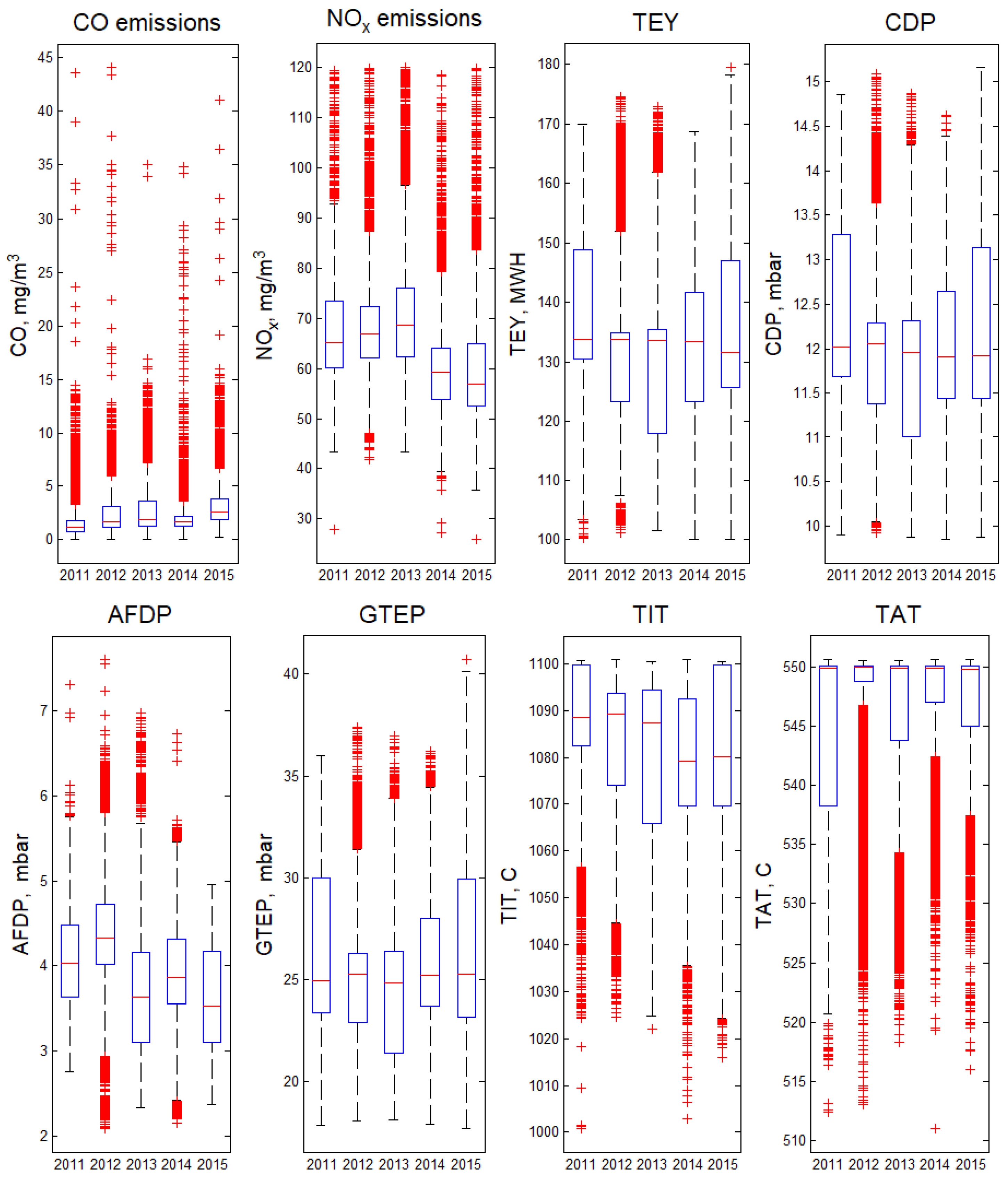
The first step in our data analysis was to answer the question of whether it is possible to consider the data for all 5 years as a single training set and build a single model, or whether it is necessary to separate the data by years or seasons. Figure 1 shows boxplots of technological process parameters and CO and NOx emissions over 5 years. Note that the median for the turbine energy yield for 2011–2014 remained practically unchanged, whilst in 2015, it decreased by 1.5%. At that, the median for CO emissions in 2015 was significantly higher than the values for previous years. For NOx emissions in 2014 and 2015, the median was lower compared to 2011–2013 by more than 10%. We cannot obtain additional information about the equipment maintenance during the period 2011–2015, but these observations allow us to conclude that to train the NOx model, it is worth dividing the data into two subsets and building one model for 2011–2013 dataset, and the second for 2014–2015.
Points marked with symbol “+” show values that are larger than or smaller than , where and are the 25th and 75th percentiles, respectively. They cannot be considered outliers if there is a simultaneous change in CO emission and process parameters. Moreover, a sharp increase in emission is a key issue for the problem under consideration. For CO emission, one can see a significant number of cases when emissions are 5–40 times greater than the median values, but the total amount of CO emissions on average is approximately 5–10% of NOx emission. Thus, CO emission can dramatically increase and it is important to indicate the situation that leads to extraordinary emissions. We divided the data into two subsets. The first subset included 10% of the data with the highest CO values (emissions exceeding 4.75 mg/m3), we called this subset “extreme CO”. For the second subset, CO emissions were less than 4.75 mg/m3, and we called this subset “standard CO”.
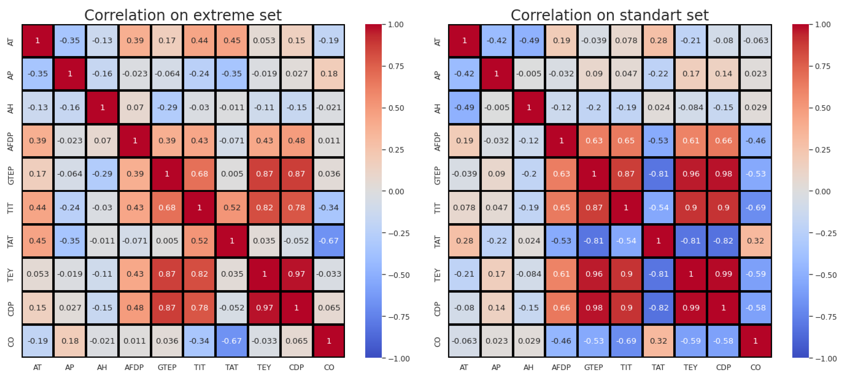
We plotted correlation matrices for the subset of extreme CO samples and for the subset of standard CO (Figure 2). Comparison of the correlation matrices aims to describe the relationship between the parameters for two subsets and to make sure that the reduction in the number of predictors does not lead to a reduction in the information needed to predict emissions.
Figure 2 shows that out of four pairs of variables with a correlation of more than 0.9 for the standard CO subset, only one pair (CDP and TEY) remained in the extreme CO subset; for different subsets, the change in the correlation coefficient between these variables was very small: = 0.99 and = 0.97. It makes no sense to use both of these variables as predictors; it is better to leave one, since the presence of the second practically adds no new information. We decided to exclude CDP since energy production TEY is a more explicable parameter.
For the CO standard set, all correlation coefficients between CO emissions and technological and ambient variables are statistically significant. For the CO extreme set, the statistically insignificant correlation coefficients are , , , , . A statistically insignificant correlation coefficient does not mean that the variables are independent, since there may be a nonlinear relationship between the variables. For standard and extreme subsets, the largest changes are for the correlation coefficients between TAT (7th row and column) and all technological parameters. The colors show the relationship of parameters and the difference is visually clear. This means that dividing all data into two subsets is justified and in this case a more accurate forecast of emissions can be obtained. Thus, we decided to build a classification model to predict the class of CO emission (extreme or standard) and develop a different model for each class.
3. Methods and Models
Thus, the classification model using the random forest algorithm [11] was constructed. The effectiveness of a classification model was determined by metrics such as , , and -score, that can be calculated as follows:
where:
- —the number of positive class predictions that actually belong to the positive class;
- —the number of positive class predictions that actually belong to the negative class;
- —the number of negative class predictions that actually belong to the positive class.
The metrics of the model are given in Table 2. The -score for extreme class identification should be improved. In Section 4, a novel method to build a classification model will be presented. This section presents models for predicting CO and NOx emissions using symbolic regression (SR).
The advantage of symbolic regression (SR) is that it allows to generate models in the form of analytic equations, and the researcher does not need to determine the structure of the model in advance. The disadvantage of the method is the long running time of the algorithm in the case of a large number of explanatory variables, the difficulty in selecting the tuning parameters, the lack of confidence that the best possible solution has been obtained, since the result depends on a variety of random events. Nevertheless, the method has found application in several practical problems. Ref. [12] presents the formulae for estimating bubble-point pressure and the formation volume factor of crude oil with four basic oil properties: temperature, gas solubility, oil API gravity and gas-specific gravity as predictors. In [13], the SR methodology was used to develop a correlation to predict thermodynamic conditions for hydrates’ formation. In [14], explicit approximations of widely used hydraulics, the Colebrook equation for flow friction obtained with SR method are considered. In [15], authors proposed two-phase bi-objective symbolic regression method and discussed how to choose the model that fit the training data as precisely as possible and is consistent with the prior knowledge about the system given in the form of nonlinear inequality and equality constraints. In [16], the authors, using SR, reconstruct the pressure and the forcing field for a weakly turbulent fluid flow only when the velocity field is known.
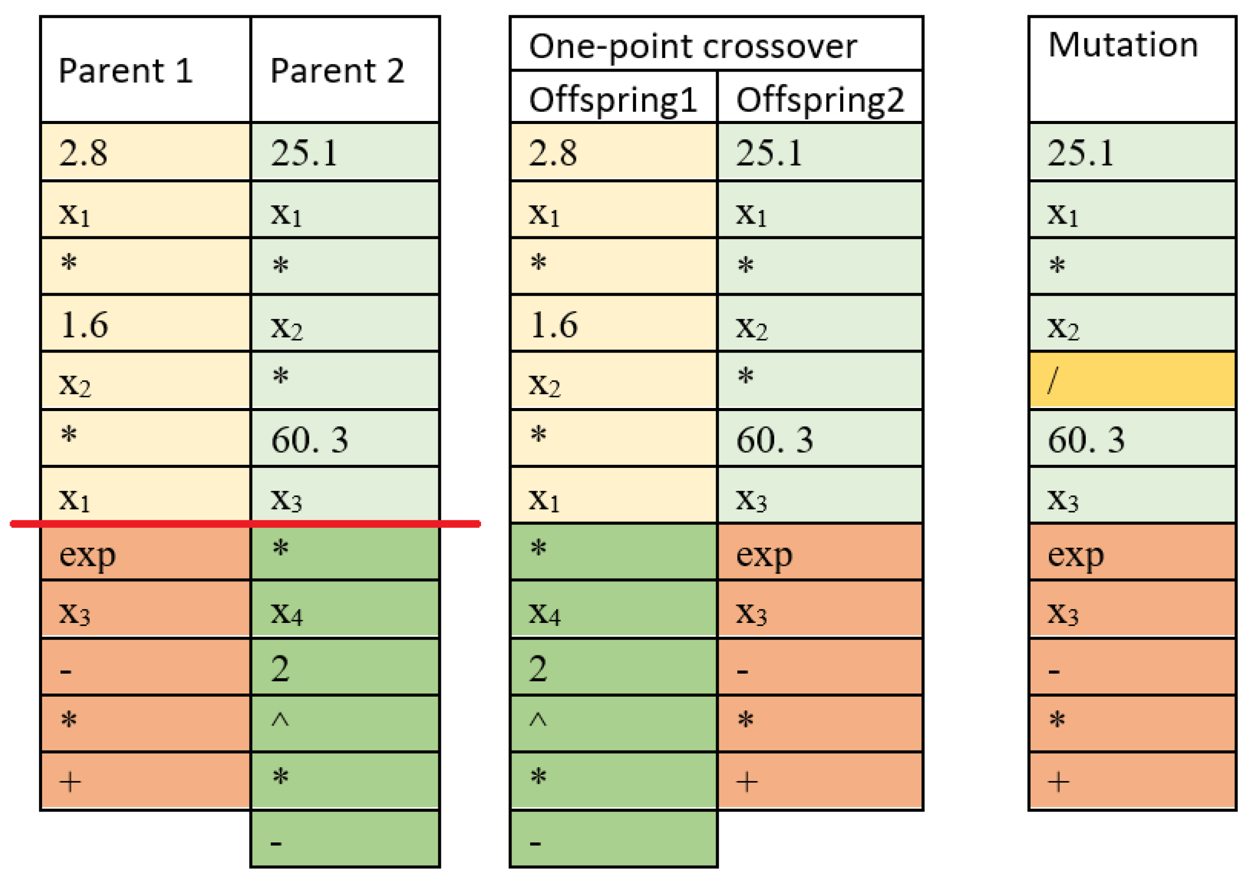
Symbolic regression uses the approach of genetic algorithm [17]. The idea of SR is to construct a model (chromosome) as a sequence of genes, as a gene can be used a predictor, a number, an arithmetic operation or a function. To avoid the use of parentheses, Polish postfix notation is used. In Figure 3, the first and second columns show two formulae below in Polish postfix notation:
The first population (certain number) of formulae, i.e., chromosomes, is randomly generated. For each chromosome, a fitness function is calculated (the sum of the squares of the differences between the observed dependent variable and the value predicted by the generated function). Then the parents are selected, and new chromosomes are created with the crossover operation. The idea behind the crossover operation is to produce offspring by exchanging sections of chromosomes. In a single-point crossing, a breakpoint in each chromosome is randomly selected. Both structures are broken into two segments at this point. Then, the corresponding segments from different parents are “glued together” and two children are obtained. In Figure 3, the crossover point (red line) divides Parent 1 (in the first column) into two fragments, marked with light yellow and terracotta colors, and Parent 2 (in the second column) into light green and green sections, so Offspring 1 (in the third column) receives a light yellow fragment from Parent 1 and a green fragment from Parent 2, and Offspring 2 (in the fourth column) receives a light green fragment from Parent 2 and a terracotta fragment from Parent 1. Thus, the formulae after the crossover operation are as follows:
The next step in the genetic programming algorithm is chromosome mutation. A mutation is the transformation of a chromosome that accidentally changes one or more of its genes. In our example in Figure 3, in the fifth column, for the second offspring, the multiplication operation was replaced by the division operation (yellow cell) as a result of the mutation. So, the second offspring is transformed as The mutation operator is designed to maintain the diversity of individuals in a population and to prevent falling into the local minimum.
Then, the fitness function for new chromosomes is calculated and the next generation is formed. The described procedure is repeated until one of the following conditions is met: the change in the best value of the fitness function becomes less than a given tolerance; a predetermined number of generations is obtained, or the maximum time to complete the calculation is reached. A detailed description of methods for parental selection and chromosome selection for a new population is beyond the scope of this article. In our study, we used free open source genetic programming and symbolic data mining MATLAB toolbox [18].
The predictors are standardized using the Z-score:
where z—standardized value of parameter x; x—original value of parameter x; —the mean value of parameter x; and —the standard deviation of parameter x.
Formulae for extreme and standard CO emissions are given below, and the coefficients are rounded to the nearest hundredth. As genes, we used four arithmetic operations, the operation of raising to an integer power, exponential and logarithmic functions and a unary minus:
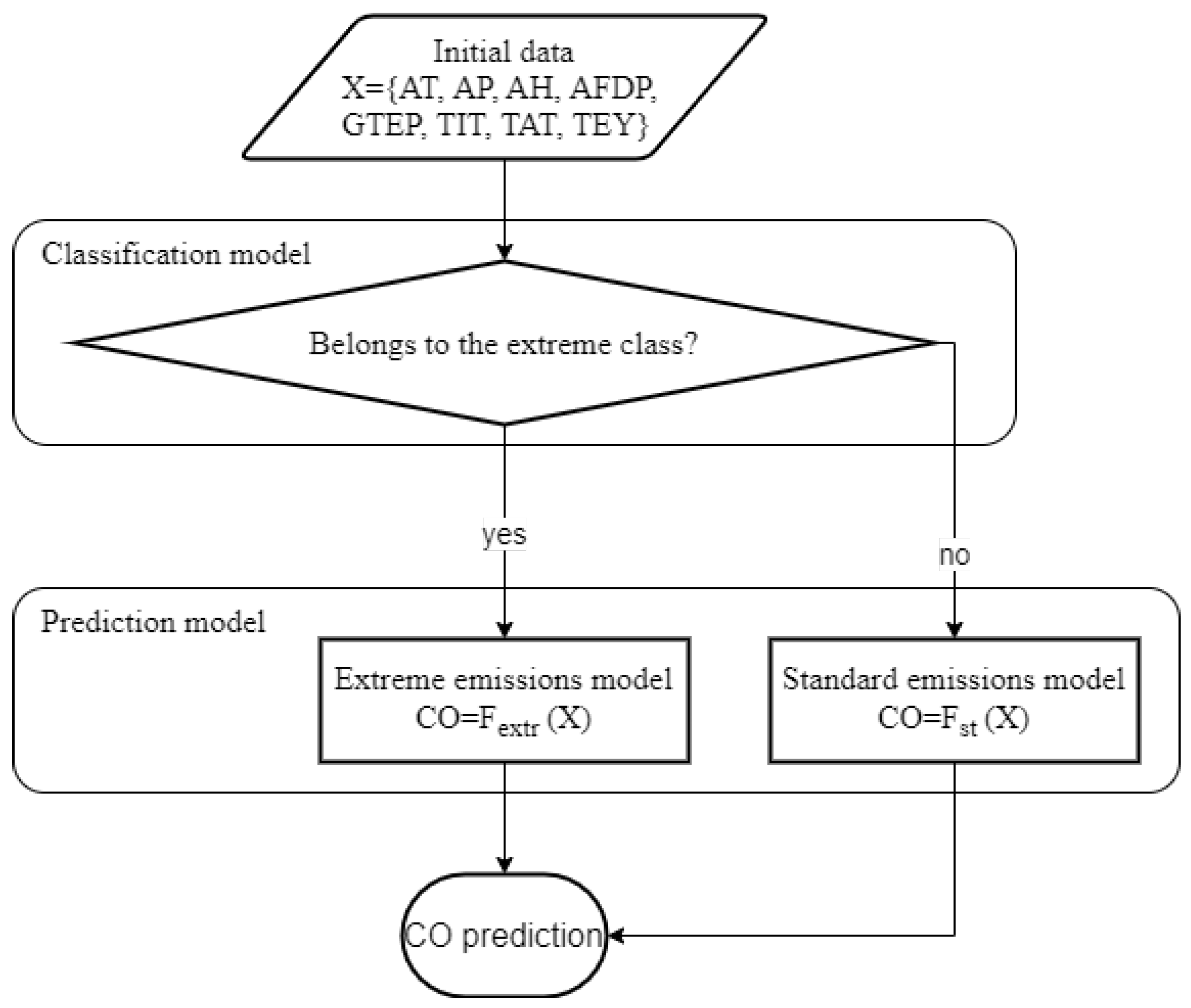
The interaction between the generated models is shown in Figure 4. Models are obtained in a convenient form, but the interpretation of the models is not always easy.
Formulae for NOx emissions obtained for subsets 2011–2013 (training set includes 15,534 samples) and 2014–2015 (training set includes 10,164 samples) are shown below:
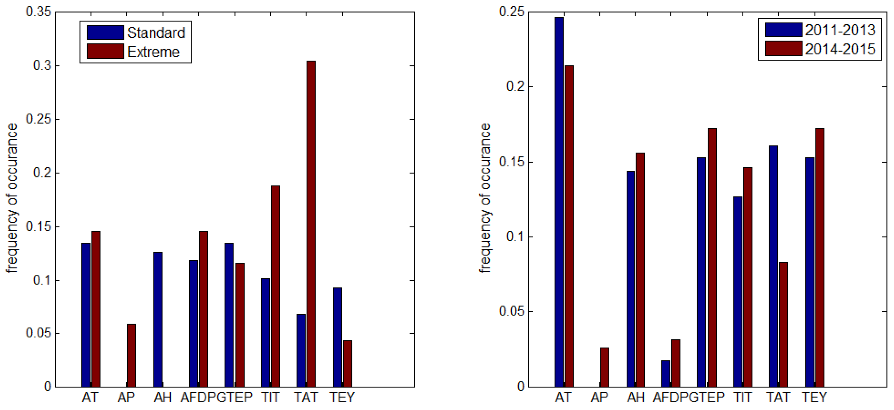
More formulae generated with the SR procedure are given in Appendix A.1, Appendix A.2 and Appendix A.3, they differ in the number and composition of the terms. The influence of the parameter can be determined by the frequency of occurrence of the corresponding variable in the formulae. We collected a set of 20 formulae for each class for CO and each subset for NO and calculated the frequency of using the input variables, which is shown in Figure 5. Some conclusions can be drawn about the importance of the parameters and features for different cases. is not included in any formula for extreme CO emission (remember the statistical insignificance of the correlation coefficient ). and are rare (the latter is not the most obvious fact, as with a sharp increase in energy production, a sharp increase in CO emissions can be expected). The most important parameter for extreme CO prediction is . For standard CO emissions, the frequencies of , , , are in the range of 0.12–0.13, followed by , and . is not present in the formulae, its role in standard CO emission prediction is negligible. For NOx emissions, we see the negligible importance of and parameters for both subsets. has the highest frequency of occurrence, , , , have roughly equal frequencies, the difference between subsets 2011–2013 and 2014–2015 is in frequency of . This fact may have a technological explanation, as we indicated in Section 2.
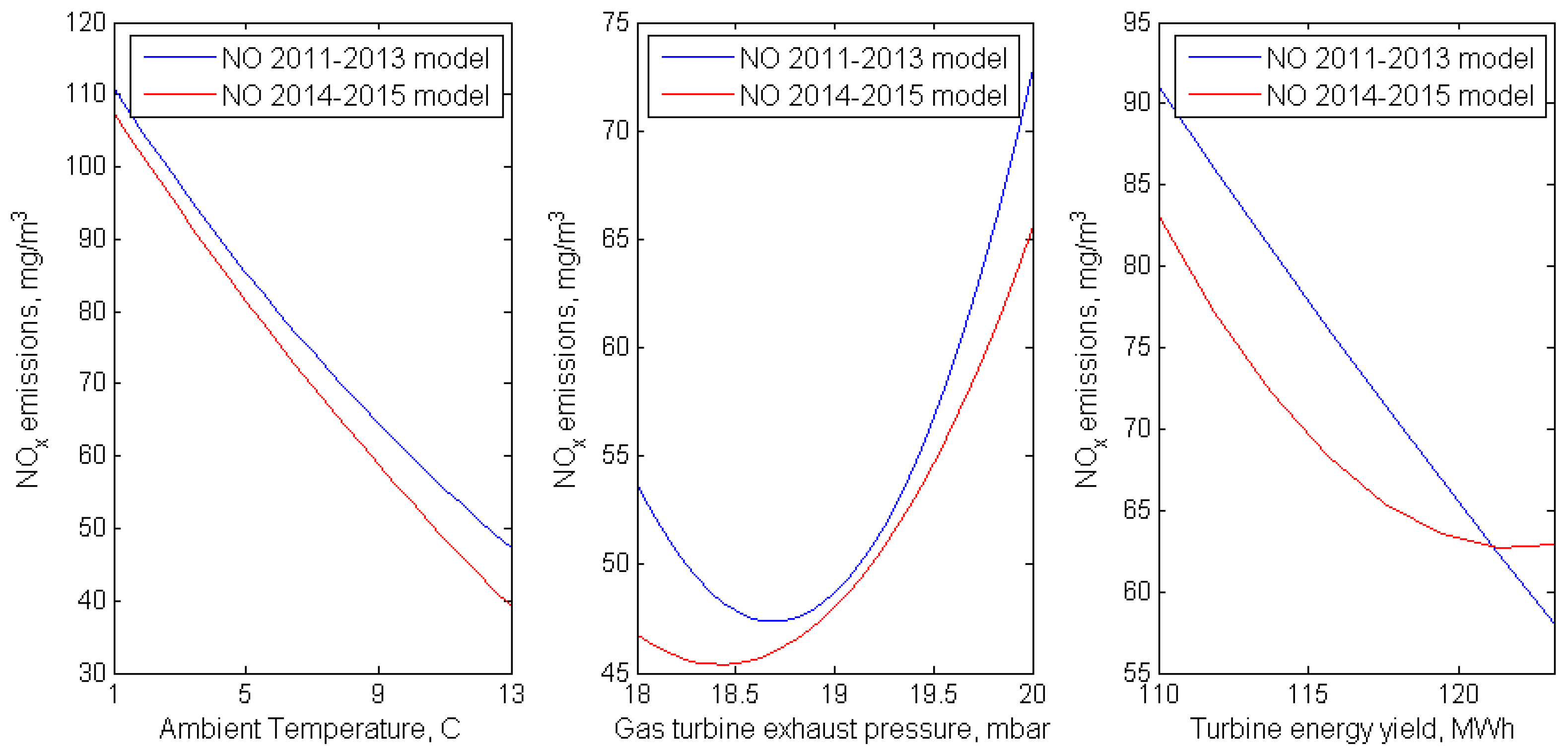
Nevertheless, it is interesting to compare the influence of some predictors on the outputs of the models for NOx emissions built for the periods of 2011–2013 and 2014–2015. Figure 6 shows graphs of NOx emissions versus AT, GTEP and TEY, with the other explanatory variables held constant. For different periods, the trend in the parameters remains; as already noted, for the period 2014–2015, NOx emissions are slightly lower than for 2011–2013 under the same conditions.
We emphasize the fact that different runs of the program can give very different formulae with approximately equal metrics for the quality of the models. One reason is that, for the dataset under consideration, a fairly large part of the variation in the dependent variables (CO and NOx emission) cannot be explained by predictors due to the large time interval for averaging the collected data (1 h). If data with a shorter time interval are available, it will be possible to continue research and obtain more accurate formulae. The resulting formulae are specific to the equipment. They will be different for different types of turbines (e.g., open cycle gas turbines or combined cycle) and even for turbines of the same type but with a different operating life. For practical tasks, it is necessary to collaborate with experts in the technological area to choose the best model that gives an acceptable quality forecast and meets the expectations of the specialists. Nevertheless, the structure of the presented models is simple and understandable, which cannot be said about the models created by random forest algorithm, or ELM, for example.
The issue of the relationship between CO and NOx emissions was mentioned in [19,20]. We calculated the correlation coefficients between CO and NOx emissions for the testing sets and the predictions of the obtained models. It should be noted that the data were collected with a fairly large time step, so the relationship between CO and NOx may differ from the real one. However, from the point of view of the consistency of the initial data and the constructed models, it is of interest to analyze the correlation of CO and NOx emissions. For the 2011–2013 period, the correlation coefficient for the dataset is , for model predictions . For the 2014–2015 period, the correlation coefficient for the dataset is , for model predictions . Thus, the difference between the two time periods can be seen, as well as the consistency of the model results. SR does not allow a model to be built with two dependent variables, but compared to the canonical correlation analysis used in [3], it provides results with a lower mean absolute error where the relationship between two dependent variables is preserved.
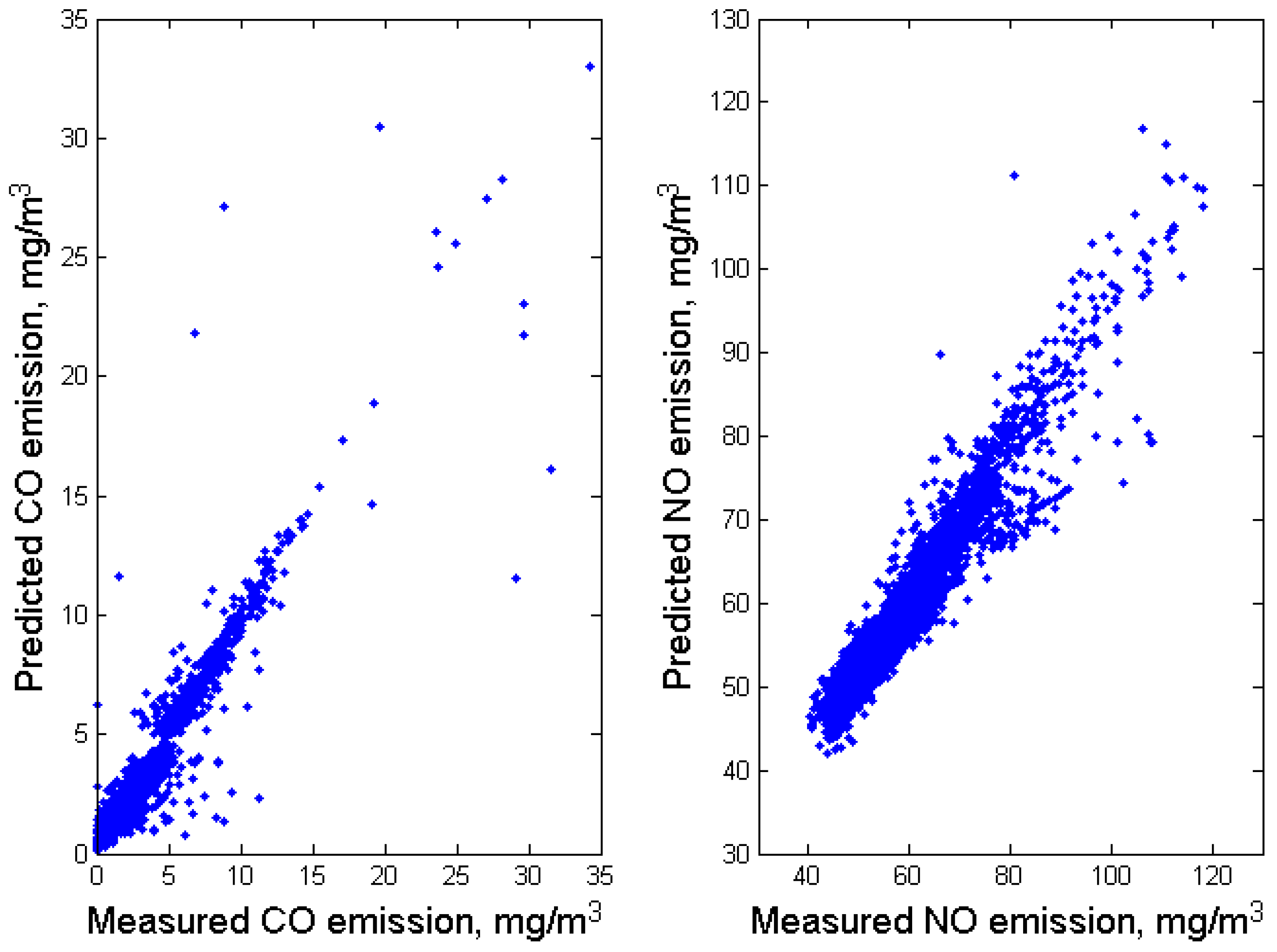
We tested the models for NOx emission with two testing sets: for 2011–2013 (which includes 6658 samples) and for 2014–2015 (which includes 4356 samples), each of which includes 30% of the data. The histograms of the predictors and dependent variables for training and testing sets are statistically identical. The results for the testing set in comparison with the measured values NOx for 2014–2015 are shown in Figure 7 on the right, the metrics are MAE = 2.5 mg/m3, . The model’s performance is better than that obtained in [3] for random forest and ELM algorithms and about as good as the results for K-nearest-neighbor method presented in [4].
We tested the models for CO emission with a testing set, which includes 11,021 samples, 1053 of them belong to the extreme class and 9968—to the standard class. The results for the testing set in comparison with the measured values CO are shown in Figure 7 on the left, the metrics are MAE = 0.39 mg/m3, . The model’s performance is better than it was obtained in [3], but there is a sharp boundary between the two intervals [0, 4.75] and (4.75, 30]. The idea of crisp presentation of the intervals leads to the fact that an emission of 4.7 mg/m3 belongs to the standard emission class and an emission of 4.8 mg/m3 belongs to the extreme emission class, therefore we decided to apply the approach based on fuzzy logic, a concept first introduced in [21].
4. Fuzzy Classification Model and Modified Symbolic Regression Model
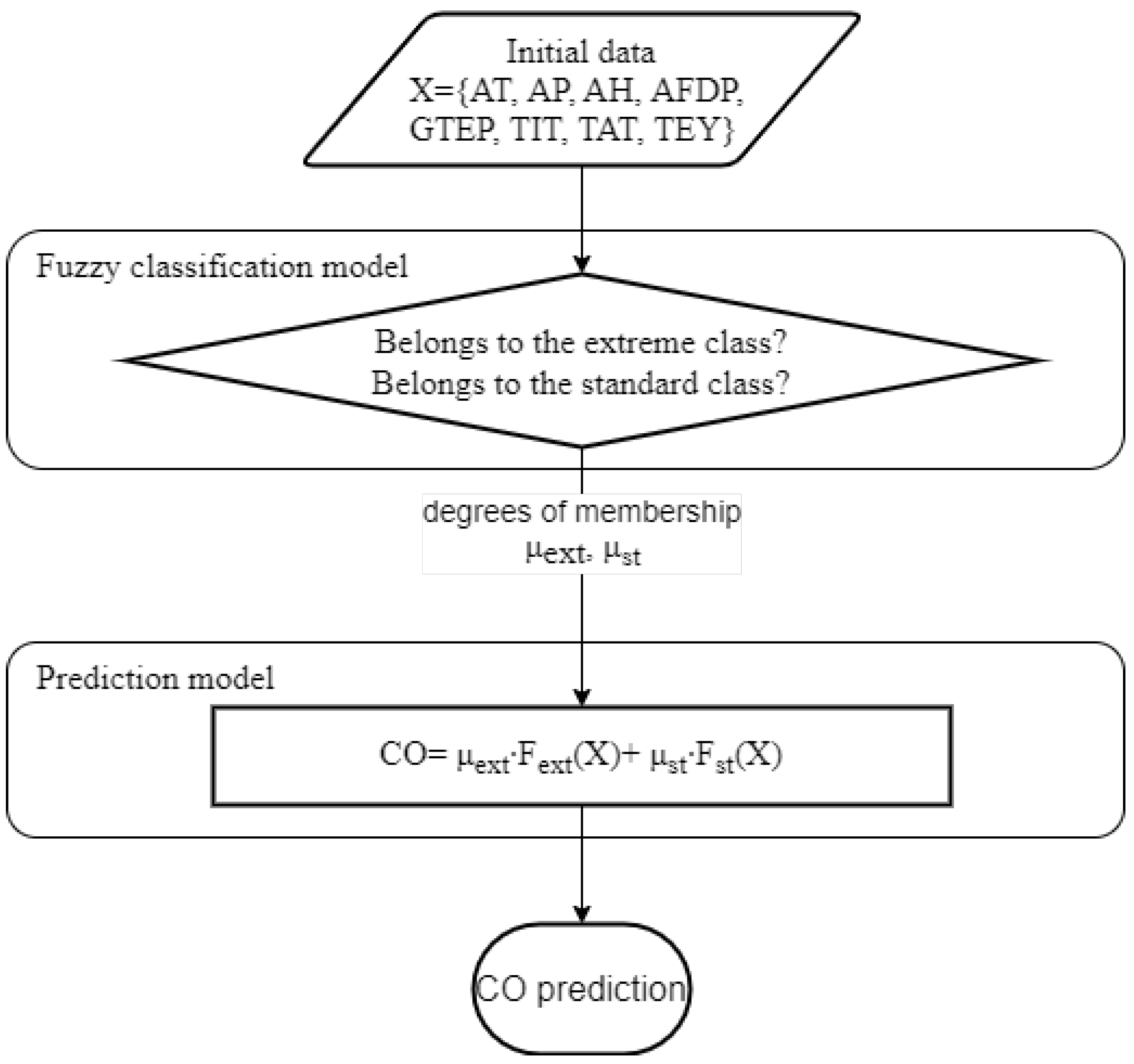
We defined an output fuzzy variable named CLASS, which includes two terms: “Standard” and “Extreme”, and developed a set of rules for determining the degree of membership to each term based on the values of the input parameters. The predicted value of CO emission is calculated similar to Sugeno algorithm [22] as follows:
where —the degree of membership to the class “Extreme”; ; is defined as a result of fuzzy reasoning; —the degree of membership to the class “Standard”; ; —CO emission, calculated using Formula (3); —CO emission calculated using Formula (4); and —predicted CO emission.
The input variables for the fuzzy inference system (FIS) were selected after analyzing the components of formulae (3), (4), (A1)–(A7), and other formulae obtained with SR. The goal was to select the components with the least similarity for samples belonging to the extreme and standard crisp subsets in the training set. Histograms of some of them are shown in Figure 8.
We selected components and defined them as input variables for FIS with two terms: “Big” and “Small”. The nonlinear S-shaped membership function with two parameters A and B describes the term “Big”. Parameter A defines the left bound of the component’s values, where the membership function equals 0, and B defines the right bound of the component’s values, where the membership function equals 1 (8):
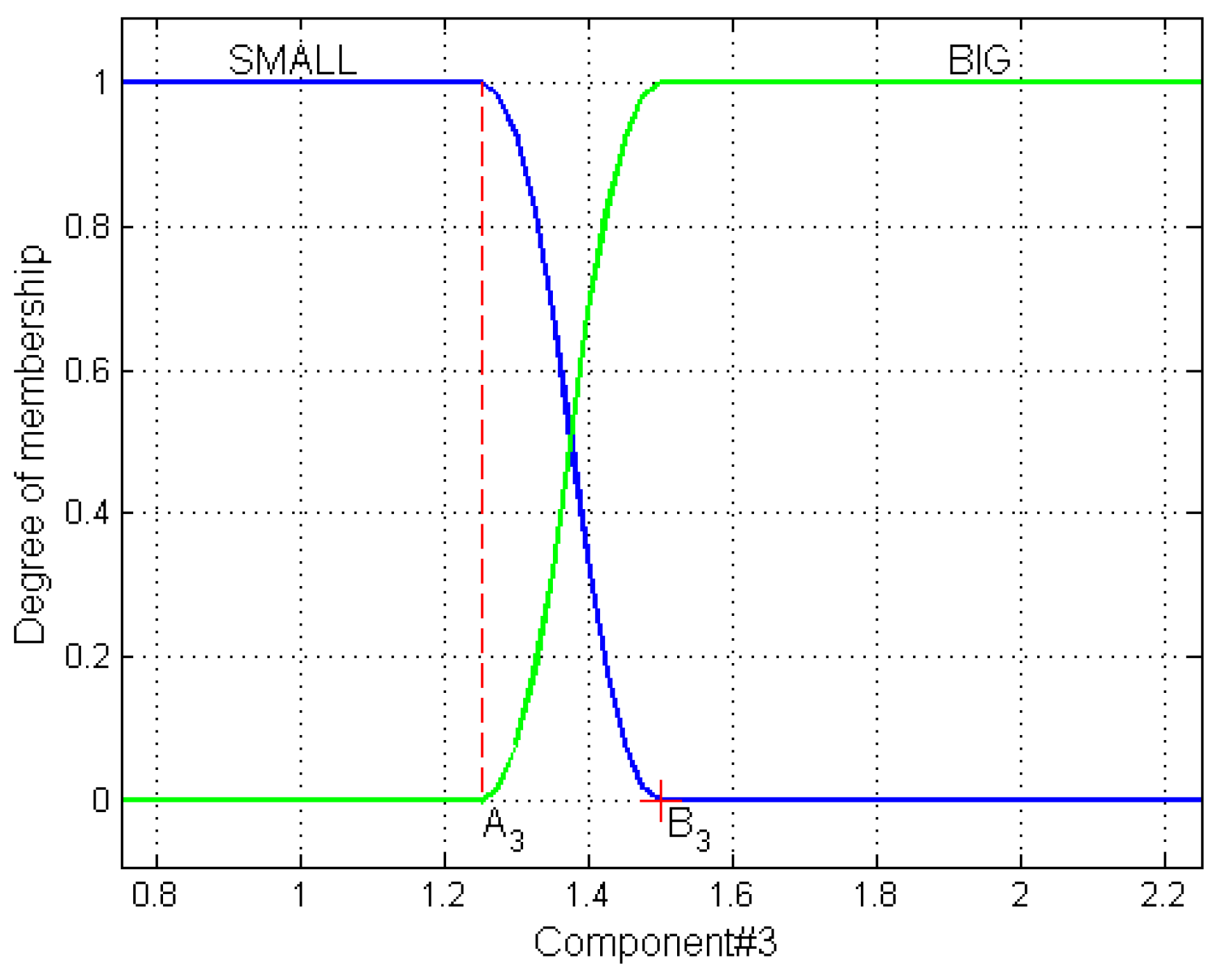
To define the term “Small”, we use a nonlinear Z-shaped membership function that is mirror symmetrical to an S-shaped one. Parameter A defines the left bound of the component’s values, where the membership function equals 1 and B defines the right bound of the component’s values where the membership function equals 0. The graphs of the nonlinear Z-shaped and S-shaped membership functions defined for Component#3 are shown in Figure 9. We chose a symmetrical way of representing the terms “Small” and “Big”, so for each component, it is enough to define only two parameters and to calculate the degree of membership to each term:
To build a fuzzy classification model, a FIS with five input variables and one output variable was constructed. The outputs of the system are two parameters and , which define the degree of membership of the sample of input values to extreme or standard classes.
We defined 11 rules in the form “IF–THEN”. An example of four rules corresponding to the components given in Figure 8 is shown below:
IF COMPONENT#1 is small CLASS is extreme;
IF COMPONENT#2 is small CLASS is extreme;
IF COMPONENT#3 is big CLASS is extreme;
IF COMPONENT#1 is big CLASS is standard.
The fuzzy output is calculated as
where —the value of membership function calculated for the vector of input data in i-th rule; n—number of rules; and —the weight of the i-th rule corresponding to its contribution of the correct decision.
Now let us consider the formulation of the constrained optimization problem to define the parameters , , from the training set. Our goal was to maximize the performance of the fuzzy classification model, namely the value of -score (1), the control parameters are: , for each component and the weights for each rule. The constraints are:
where —the values of the j-th component calculated from the training set.
We used a genetic algorithm [17], implemented as a standard function in MATLAB. The hyperparameters are:
- Population size is 150;
- Selection is tournament;
- Single point crossover, crossover fraction is 0.8;
- Uniform mutation, mutation rate 0.01.
Each chromosome is a set of variables , fitness function is the value of the -score for the training set, to calculate it we used -cut to transform the obtained fuzzy sets into the crisp sets. Thus, we obtained the optimal set of FIS parameters which gives the highest value for the -score of the training set, and then we can determine the degree of membership for the extreme and the standard classes for any sample of input data.
The metrics for the obtained fuzzy classification model for a testing set are given in Table 3. As one can see, the metrics are slightly better compared to the first crisp classification model Table 2. To test fuzzy classification model and to calculate -score for the testing set, we transformed fuzzy subsets to crisp ones, but our goal is to use the advantages of the fuzzy logic approach, and use the degrees of membership to each class to obtain a better prediction for CO emission. The flowchart of the algorithm is given in Figure 10.
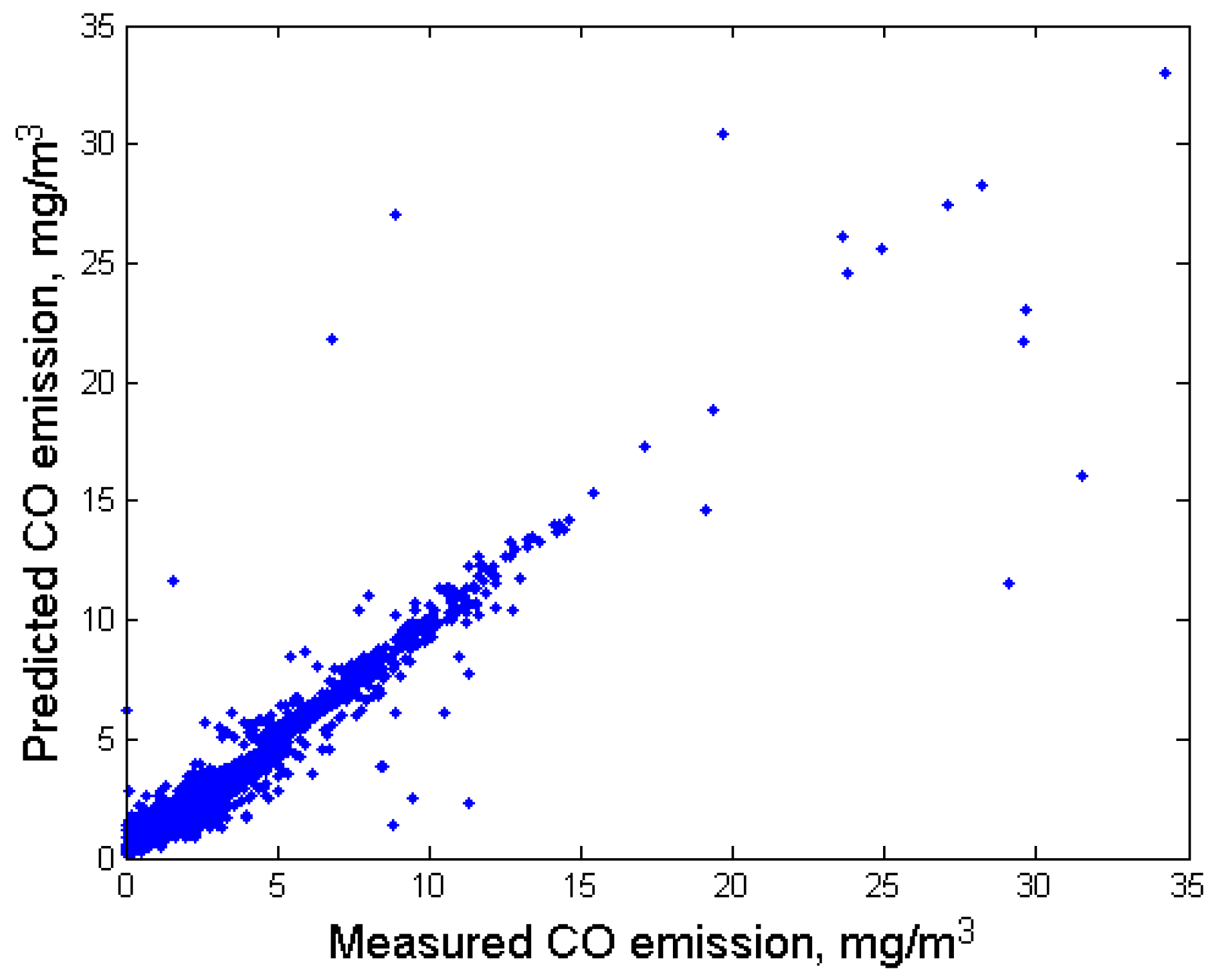
Figure 11 shows predicted and measured CO emissions for the testing set using fuzzy classification model and SR formulae (3) and (4). The metrics are MAE = 0.27 mg/m3, . Compared to the previous model (see Figure 7), one can notice that the points are better grouped around a line, the sharp transition between the areas where there was a boundary between classes disappeared. Approximately 10 points are located at a significant distance from the line; in these cases, the prediction error is large, which can be explained by the large time interval (1 h) when forming the input data vector.
5. Conclusions
This paper presents a study of an open dataset on CO and NOx emissions from gas turbines. To predict CO emissions, it is proposed to use a combined model that includes symbolic regression models for the standard and extreme classes and a fuzzy classification model which makes it possible to determine the degree of membership to each class for the vector of input parameters. The paper describes a fuzzy classification model and shows how the input variables for a fuzzy inference system are formed. For the first time, it is proposed to investigate the components of formulae generated by the symbolic regression method for defining the differing characteristics of classes. The obtained metrics of the models exceed the indicators presented in previous works. It should be noted that the available dataset with a frequency of 1 h does not allow for the full use of the presented models for predictive monitoring systems; it would be interesting to continue the study, if possible, to investigate the operation of the proposed algorithms for data with a shorter interval between measurements.
Author Contributions
Conceptualization, O.K.; methodology, O.K.; software, O.K., K.N.; validation, O.K., K.N.; formal analysis, O.K.; investigation, O.K., K.N.; writing—original draft preparation, O.K., K.N.; writing—review and editing, O.K., K.N.; visualization, O.K., K.N. All authors have read and agreed to the published version of the manuscript.
Funding
This research received no external funding.
Data Availability Statement
This study used an open dataset; the links are provided in the bibliography.
Acknowledgments
The authors are grateful to Heysem Kaya, Pınar Tüfekci and Erdinç Uzun for providing the publicly available dataset. The authors thank the reviewers and editors for their work.
Conflicts of Interest
The authors declare no conflict of interest.
Abbreviations
The following abbreviations are used in this manuscript:
| PEMS | predictive emission monitoring systems |
| CEMS | continuous emission monitoring systems |
| MAE | mean absolute error |
| FIS | fuzzy inference system |
| ELM | extreme learning machine |
| MLR | multiple linear regression |
| CCA | canonical correlation analysis |
Appendix A. Symbolic Regression Formulae for CO and NO Emissions
Appendix A.1. Formulae for Extreme CO Emissions Class
Appendix A.2. Formulae for Standard CO Emissions Class
Appendix A.3. Formulae for NO Emissions
References
- Si, M.; Tarnoczi, T.J.; Wiens, B.M.; Du, K. Development of Predictive Emissions Monitoring System Using Open Source Machine Learning Library—Keras: A Case Study on a Cogeneration Unit. IEEE Access 2019, 7, 113463–113475. [Google Scholar] [CrossRef]
- Dua, D.; Graff, C. UCI Machine Learning Repository. Available online: http://archive.ics.uci.edu/ml (accessed on 10 October 2021).
- Kaya, H.; Tüfekci, P.; Uzun, E. Predicting CO and NOx emissions from gas turbines: Novel data and a benchmark PEMS. Turk. J. Electr. Eng. Comput. Sci. 2019, 27, 4783–4796. [Google Scholar] [CrossRef]
- Rezazadeh, A. Environmental Pollution Prediction of NOx by Process Analysis and Predictive Modelling in Natural Gas Turbine Power Plants. Pollution 2021, 7, 481–494. [Google Scholar]
- Si, M.; Du, K. Development of a predictive emissions model using a gradient boosting machine learning method. Environ. Technol. Innov. 2020, 20, 101028. [Google Scholar] [CrossRef]
- Chawathe, S.S. Explainable Predictions of Industrial Emissions. In Proceedings of the 2021 IEEE International IOT, Electronics and Mechatronics Conference (IEMTRONICS), Toronto, ON, Canada, 21–24 April 2021; pp. 1–7. [Google Scholar]
- Nino-Adan, I.; Portillo, E.; Landa-Torres, I.; Manjarres, D. Normalization Influence on ANN-Based Models Performance: A New Proposal for Features’ Contribution Analysis. IEEE Access 2021, 9, 125462–125477. [Google Scholar] [CrossRef]
- Etemadi, S.; Khashei, M. Etemadi multiple linear regression. Measurement 2021, 186, 110080. [Google Scholar] [CrossRef]
- Manasis, C.; Assimakis, N.; Vikias, V.; Ktena, A.; Stamatelos, T. Power Generation Prediction of an Open Cycle Gas Turbine Using Kalman Filter. Energies 2020, 13, 6692. [Google Scholar] [CrossRef]
- Giunta, G.; Vernazza, R.; Salerno, R.; Ceppi, A.; Ercolani, G.; Mancini, M. Hourly weather forecasts for gas turbine power generation. Meteorol. Z. 2017, 26, 307–317. [Google Scholar] [CrossRef]
- Breiman, L. Random forests. Mach. Learn. 2001, 45, 5–32. [Google Scholar] [CrossRef] [Green Version]
- Abooali, D.; Khamehchi, E. Toward predictive models for estimation of bubble-point pressure and formation volume factor of crude oil using an intelligent approach. Braz. J. Chem. Eng. 2016, 33, 1083–1090. [Google Scholar] [CrossRef] [Green Version]
- Khan, S.H.; Kumari, A.; Dixit, G.; Majumder, C.B.; Arora, A. Thermodynamic modeling and correlations of CH4, C2H6, CO2, H2S, and N2 hydrates with cage occupancies. J. Petrol. Explor. Prod. Technol. 2020, 10, 3689–3709. [Google Scholar] [CrossRef]
- Praks, P.; Brkić, D. Symbolic Regression-Based Genetic Approximations of the Colebrook Equation for Flow Friction. Water 2018, 10, 1175. [Google Scholar] [CrossRef] [Green Version]
- Kubalík, J.; Derner, E.; Babuška, R. Multi-objective symbolic regression for physics-aware dynamic modeling. Expert Syst. Appl. 2021, 182, 115210. [Google Scholar] [CrossRef]
- Reinbold, P.A.K.; Kageorge, L.M.; Schatz, M.F.; Grigoriev, R.O. Robust learning from noisy, incomplete, high-dimensional experimental data via physically constrained symbolic regression. Nat. Commun. 2021, 12, 3219. [Google Scholar] [CrossRef] [PubMed]
- Mitchell, M. An Introduction to Genetic Algorithms; MIT Press: Cambridge, MA, USA, 1996; p. 205. [Google Scholar]
- Searson, D. GPTIPS–Free Open-Source Genetic Programming and Symbolic Data Mining MATLAB Toolbox. Available online: https://sites.google.com/site/gptips4matlab/ (accessed on 27 September 2021).
- Krzywanski, J.; Czakiert, T.; Shimizu, T.; Majchrzak-Kuceba, I.; Shimazaki, Y.; Zylka, A.; Grabowska, K.; Sosnowski, M. NOx Emissions from Regenerator of Calcium Looping Process. Energy Fuels 2018, 32, 6355–6362. [Google Scholar] [CrossRef]
- Gungor, A. Simulation of NOx Emission in Circulating Fluidized Beds Burning Low-grade Fuels. Energy Fuels 2009, 23, 2475–2481. [Google Scholar] [CrossRef]
- Zadeh, L.A. Fuzzy logic and approximate reasoning. Synthese 1975, 30, 407–428. [Google Scholar] [CrossRef]
- Takagi, T.; Sugeno, M. Fuzzy identification of systems and its applications to modeling and control. IEEE Trans. Syst. Man Cybernet. 1985, 15, 116–132. [Google Scholar] [CrossRef]
Figure 1.
Boxplots of the process parameters and CO and NOx emissions over 5 years.

Figure 2.
Correlation matrices for the CO extreme set and CO standard set.

Figure 3.
An example of one-point crossover and mutation operators.

Figure 4.
Flowchart for CO prediction with crisp classification model.

Figure 5.
The frequency of occurrence of input parameters in symbolic regression models.

Figure 6.
Impact of AT, GTEP and TEY on the NO emissions model results.

Figure 7.
Predicted and measured CO (on the left) and NOx (on the right) emissions for the testing set.
Figure 7.
Predicted and measured CO (on the left) and NOx (on the right) emissions for the testing set.

Figure 8.
Histograms of COMPONENT#1 ; COMPONENT#2 ; and COMPONENT#3 .

Figure 9.
Membership functions for terms “Small” and “Big” and their parameters.

Figure 10.
Flowchart for CO prediction with the fuzzy classification model.

Figure 11.
Predicted and measured CO emissions for the testing set for the SR model based on fuzzy classification.
Figure 11.
Predicted and measured CO emissions for the testing set for the SR model based on fuzzy classification.


Table 1.
The list of process parameters.
| Process Parameters | Abbreviation | Unit |
|---|---|---|
| Air filter difference pressure | AFDP | mbar |
| Gas turbine exhaust pressure | GTEP | mbar |
| Turbine inlet temperature | TIT | °C |
| Turbine after temperature | TAT | °C |
| Turbine energy yield | TEY | MWh |
| Compressor discharge pressure | CDP | mbar |
Table 2.
Metrics for random forest classification model.
| Class | Precision | Recall | -Score | Support |
|---|---|---|---|---|
| Standard | 0.981 | 0.974 | 0.977 | 9968 |
| Extreme | 0.804 | 0.757 | 0.779 | 1053 |
Table 3.
Metrics for fuzzy classification model.
| Class | Precision | Recall | -Score | Support |
|---|---|---|---|---|
| Standard | 0.984 | 0.975 | 0.979 | 9968 |
| Extreme | 0.836 | 0.767 | 0.800 | 1053 |
Publisher’s Note: MDPI stays neutral with regard to jurisdictional claims in published maps and institutional affiliations. |
© 2021 by the authors. Licensee MDPI, Basel, Switzerland. This article is an open access article distributed under the terms and conditions of the Creative Commons Attribution (CC BY) license (https://creativecommons.org/licenses/by/4.0/).
Share and Cite
MDPI and ACS Style
Kochueva, O.; Nikolskii, K. Data Analysis and Symbolic Regression Models for Predicting CO and NOx Emissions from Gas Turbines. Computation 2021, 9, 139. https://0-doi-org.brum.beds.ac.uk/10.3390/computation9120139
AMA Style
Kochueva O, Nikolskii K. Data Analysis and Symbolic Regression Models for Predicting CO and NOx Emissions from Gas Turbines. Computation. 2021; 9(12):139. https://0-doi-org.brum.beds.ac.uk/10.3390/computation9120139
Chicago/Turabian StyleKochueva, Olga, and Kirill Nikolskii. 2021. "Data Analysis and Symbolic Regression Models for Predicting CO and NOx Emissions from Gas Turbines" Computation 9, no. 12: 139. https://0-doi-org.brum.beds.ac.uk/10.3390/computation9120139
Note that from the first issue of 2016, this journal uses article numbers instead of page numbers. See further details here.